Interest rate model risk: an overview doc
Bạn đang xem bản rút gọn của tài liệu. Xem và tải ngay bản đầy đủ của tài liệu tại đây (179.84 KB, 26 trang )
Interest rate model risk: an overview
Rajna Gibson, FrancËois-Serge Lhabitant, Nathalie Pistre, and
Denis Talay
Model risk is becoming an increasingly important concept not only in ®nancial
valuation but also for risk management issues and capital adequacy purposes. Model
risk arises as a consequence of incorrect modeling, model identi®cation or speci®cation
errors, and inadequate estimation procedures, as well as from the application of
mathematical and statistical properties of ®nancial models in imperfect ®nancial
markets. In this paper, the authors provide a de®nition of model risk, identify its
possible origins, and list the potential problems, before ®nally illustrating some of its
consequences in the context of the valuation and risk management of interest rate
contingent claims.
1. INTRODUCTION
The concept of risk is central to players in capital markets. Risk management is
the set of procedures, systems, and persons used to control the potential losses of
a ®nancial institution. The explosive increase in interest rate volatility in the late
1970s and early 1980s has produced a revolution in the art and science of
interest rate risk management. For instance, in the US, in 1994, interest rates
rose by more than 200 basis points; in 1995, there were important nonparallel
shifts in the yield curve. Complex hedging tools and techniques were developed,
and dozens of plain vanilla and exotic derivative instruments were created to
provide the ability to create customized ®nancial instruments to meet virtually
any ®nancial target exposure.
Recent crises in the derivatives markets have raised the question of interest
rate risk management. It is important for bank managers to recognize the
economic value and resultant risks related to interest rate derivative products,
including loans and deposits with embedded options. It is equally important
for regulators to measure interest rate risk correctly. This explains why the
Basle Committee on Banking Supervision (1995, 1997) issued directives to
help supervisors, shareholders, CFOs and managers in evaluating the interest
rate risk of exchange-traded and over-the-counter derivative activities of banks
and securities ®rms, including o-balance-sheet items. Under these directives,
banks are allowed to choose between using a standardized (build ing block)
approach or their own risk measurement models to calculate their value-at-
risk, which will then determine their capital charge. No particular type of
37
model is prescribed, as long as each model captures all the risks run by an
institution.
1
Many banks and ®nancial institutions already base their strategic tactical
decisions for valuation, market-making, arbitrage, or hedging on internal
models built by scientists. Extending these models to compute their value-at-
risk and resulting capital requirement may seem pretty straightforward. But we
all know that any model is by de®nition an imperfect simpli®cation, a
mathematical representation for the purposes of replicating the real world. In
some cases, a model will produce results that are sucien tly close to reality to be
adopted; but in others, it will not. What will happen in such a situation? A large
number of highly reputable banks and ®na ncial institutions have already
suered from extensive losses due to undue reliance on faulty models. For
instance,
2
in the 1970s, Merrill Lynch lost $70 milli on in the stripping of US
government bonds into `interest-only' and `principal-only' securities. Rather
than using an annuity yiel d curve to price the interest-only securities and a zero-
coupon curve to price the principal-only securities, Merrill Lynch based its
pricing on a single 30-year par yield, resulting in strong pricing biases that were
immediately arbitraged by the market at the issue. In 1992, JP Morgan lost $200
million in the mortgage-backed securities market due to an inadequate model-
ization of the prepayments. In 1997, NatWest Markets announced that mis-
pricing on sterling interest rate options had cost the bank £90 million. Traders
were selling interest rate caps and swaptions in sterling and Deutschmarks at a
wrong price, due to a naive volatility input in their systems. When the problem
was identi®ed and corrected, it resulted in a substantial downward reevaluation
of the positions. In 1997, Bank of Tokyo-Mitsubishi had to write o $83 million
on its US interest rate swaption book becau se of the application of an
inadequate pricing model: the bank was calibrating a simple Black±Derman±
Toy model with at-the-money swaptions, leading to a systematic pricing bias for
out-of-the-money and Bermuda swaptions.
The problem is not limited to the interest rate contingent claims market. It
also exists, for instance, in the stock market. In Risk magazine, the late Fisher
Black (1990) commented: ``I sometimes wonder why people still use the Black
and Scholes formula, since it is based on such sim ple assumptionsÐunrealistic-
ally simple assumptions.'' The answer can be found in his 1986 presidential
allocution at the American Finance Association, where he said: ``In the end, a
theory is accepted not because it is con®rmed by conventional empirical tests,
but because researchers persuade one another that the theory is correct and
relevant.''
1
Since supervisory authorities are aware of model risk associated with the use of internal models,
they have, as a precautionary device, imposed adjustment factors: the internal model value-at-risk
should be multiplied by an adjustment factor subject to an absolute minimum of 3, and a plus
factorÐranging from 0 to 1Ðwill be added to the multiplication factor if backtesting reveals
failures in the internal model. This overfunding solution is nothing else than an insurance or an ad
hoc safety factor against model risk.
2
These events are discussed in more detail in Paul-Choudhury (1997).
Volume 1/Number 3
R. Gibson et al.38
Why did we focus on interest rate models rather than on stock models? First,
interest rate models are more complex, since the eective underlying variableÐ
the entire term structure of interest ratesÐis not observable. Second, there exists
a wider set of de rivative instruments. Third, interest rate contingent claims have
certainly generated the most abundant theoretical literature on how to price and
hedge, from the simplest to the most complex instrument, and the set of models
available is proli®c in variety and underlying assumptions. Fourth, almost every
economic agent is exposed to interest rate risk, even if he does not manage a
portfolio of securities.
Despite this, as we shall see, the literature on model risk is rather sparse
and often focuses on speci®c pricing or implied volatility ®tting issues. We
believe there are much more challenging issues to be explored. For instance, is
model risk symmetric? Is it priced in the market? Is it the source of a larger
bid±ask spread? Does it result in overfunding or underfunding of ®nancial
institutions?
In this paper, we shall provide a de ®nition of model risk and examine some of
its origins and consequences. The paper is structured as follows. Section 2
de®nes model risk, while Section 3 reviews the steps of the model-building
process which are at the origin of model risk. Section 4 exposes various
examples of model risk in¯uence in areas such as pricing, hedging, or regulatory
capital adequacy issues. Finally, Section 5 draws some conclusions.
2. MODEL RISK: SOME DEFINITIONS
As postulated by Derman (1996a, b), most ®nancial models fall into one of the
following categories:
à
Fundamental models, which are based on a set of hypotheses, postulates, and
data, together with a means of drawing dynamic inferences from them. They
attempt to build a fundamental description of some instruments or phenom-
enon. Good examples are equilibrium pricing models, which rely on a set of
hypotheses to provide a pricing formula or methodology for a ®nancial
instrument.
à
Phenomenological models, which are analogies or visualizations that describe,
represent, or help understand a phenomenon which is not directly observable.
They are not necessarily true, but provide a useful picture of the reality. Good
examples are single-factor interest rate models, which look at reality `las if'
everybody was concerned only with the short-term interest rate, whose
distribution will remain normal or lognormal at any point in time.
à
Statistical models, which generally result from a regression or best ®t between
dierent data sets. They rely on correlation rather than causation and
describe tendencies rather than dynamics. They are often a useful way to
report information on data and their trends.
Volume 1/Number 3
Interest rate model risk: an overview 39
In the following, we shall mainly focus on models belonging to the ®rst and
second categories, but we could easily extend our framework to include
statistical models. In any problem, once a fundamental model has been selected
or developed, there are typically three main sources of uncertainty:
à
Uncertainty about the model struct ure: did we specify the right model? Even
after the most diligent model-selection process, we cannot be sure that the
true modelÐif anyÐhas been selected.
à
Uncertainty about the estimates of the model parameters, given the model
structure. Did we use the right estimator?
à
Uncertainty about the application of the model in a speci®c situation, given
the model structure and its parameter estimation. Can we use the model
extensively? Or is it restricted to speci®c situations, ®nancial assets, or
markets?
These three sources of uncertainty constitute what we call model risk. Model
risk results from the inappropriate speci®cation of a theoretical model or the use
of an appropriate model but in an inadequate framework or for the wrong
purpose. How can we measure it? Should we use the dispersion, the worst case
loss, a percentile, or an extreme loss value function and minimize it? There is a
strong need for model risk understanding and measurement.
The academic literature has essentially focused on estimation risk and
uncertainty about the model use, but not on the uncertainty about the model
structure. Some exceptions are:
à
The time series analysis literatureÐsee, for instance, the collection of papers
by Dijkstra (1988)Ðas well as some econometric problems, where a model is
often selected from a large class of models using speci®c criteria such as the
largest R
2
, AIC, BIC, MIL, C
P
,orC
L
proposed by Akaike (1973), Mallows
(1973), Schwarz (1978), and Rissanen (1978), respectively. These methods
propose to select from a collection of parametric models the model which
minimizes an empirical loss (typically measured as a squared error or a minus
log-likelihood) plus some penalty term which is proportional to the dimen-
sion of the model.
à
The option-pricing literature, such as Bakshi, Cao, and Chen (1997) or
Buhler, Uhrig-Homburg, Walter, and Weber (1999), where prices resulting
from the application of dierent models and dierent input parameter
estimations are compared with quoted market prices in order to determine
which model is the `best' in terms of market calibration.
This sparseness of the literature is rather surprising, since errors arising from
uncertainty about the model structure are a priori likely to be much larger than
those arising from estimation errors or misuse of a given model.
Volume 1/Number 3
R. Gibson et al.40
3. THE STEPS OF THE MODEL BUILDING PROCESS (OR HOW
TO CREATE MODEL RISK)
In this section, we will focus on the model-building process (or the model-
adoption process, if the problem is to select a model from a set of possible
candidates) in the particular case of interest rate models. Our problem is the
following: we want to develop (or select), estimate, and use a model that can
explain and ®t the term structure of interest rates in order to price or manage a
given set of interest rate contingent securities. Our model building process can be
decomposed into four steps: identi®cation of the relevant factors, speci®cation
of the dynamics for each factor, parameter estimation, and implementation
issues.
3.1 Environment Characterization and Factor Identi®cation
The ®rst step in the model-building process is the characterization of the
environment in which we are going to operate. What does the world look like?
Is the market frictionless? Is it liquid enough? Is it complete? Are all prices
observable? Answers to these questions will often result in a set of hypotheses
that are fundamental for the model to be developed. But if the model world
diers too much from the true world, the resulting model will be useless. Note
that, on the other hand, if most economic agents adopt the model, it can become
a self-ful®lling prophecy.
The next step is the identi®cation of the factors that are driving the interest
rate term structure. This step involves the identi®cation of both the number of
factors and the factors themselves.
Which methodology should be followed? Up to now, the discussion has been
based on the assumption of the existence of a certain number of factors.
Nothing has been said about what a factor is (or how many of them are
needed)! Basically, two dierent empirical approaches can be used (see Table 1).
On the one hand, the explicit approach assumes that the factors are known and
that their returns are observed; using time series analysis, this allows us to
estimate the factor exposures.
3
On the other hand, the implicit approach is
neutral with respect to the nature of the factors and relies purely on statistical
methods, such as principal components or cluster analysis, in order to determine
a ®xed number of unique factors such that the covariance matrix of their returns
is diagonal and they maximize the explanation of the variance of the returns on
some assets. Of course, the implicit approach is frequently followed by a second
step, in which the implicit factors are compared with existing macroeconomic or
®nancial variables in order explicitly to identify them.
For instance, most empirical studies using a principal component analysis
have decomposed the motion of the interest rate term structure into three
3
An alternative is to assume that the exposures are known, which then allows us to recover cross-
sectionally the factor returns for each period.
Volume 1/Number 3
Interest rate model risk: an overview 41
independent and noncorrelated factors (see e.g. Wilson 1994):
à
The ®rst one is a shift of the term structure, i.e. a parallel movement of all the
rates. It usually accounts for up to 80±90% of the total variance (the exact
number depending on the market and on the period of observation).
à
The second one is a twist, i.e. a situation in which long-term and short-term
rates move in opposite directions. It usually accounts for an additional
5±10% of the total variance.
à
The third one is called a butter¯y (the intermediate rate moves in the opposite
direction to the short- and long-term rates). Its in¯uence is generally small
(1±2% of the total variance).
As the ®rst component generally explains a large fraction of the yield curve
movements, it may be tempting to reduce the problem to a one-factor model,
4
generally chosen as the short-term rate. Most early interest rate models (such as
Merton 1973, Vasicek 1977, Cox, Ingers oll, and Ross 1985, Hull and White
1990, 1993, etc.) are in fact single-factor models. These models are easy to
TABLE 1. Identification of factors, and comparison of explicit and implicit approaches.
Determination of factors
The goal is to summarize and/or explain the available information (for instance, a large
number of historical observations) with a limited set of factors (or variables) while
losing as little information as possible.
Implicit method Explicit method
Analyze the data over a speci®c time
span to determine simultaneously the
factors, their values, and the exposures
to the factors. Each factor is a variable
with the highest possible explanatory
power.
Specify a set of variables that are
thought to capture systematic risk, such
as macroeconomic, ®nancial, or ®rm
characteristics. It is assumed that the
factor values are observable and
measurable.
Endogenous speci®cation Exogenous speci®cation
Factors are extracted from the data and
do not have any economic interpreta-
tion
Factors are speci®ed by the user and are
easily interpreted
Neutral with respect to the nature of
the factors
Strong bias with respect to the nature of
the factors; in particular, omitting a
factor is easy.
Relying on pure statistical analysis
(principal components, cluster analysis)
Relying on intuition
Best possible ®t within the sample of
historical observations (e.g. for histor-
ical analysis)
May provide a better ®t out of the
sample of historical observations (e.g.
for forecasting)
4
It must be stressed at this point that this does not necessarily imply that the whole term structure is
forced to move in parallel, but simply that one single source of uncertainty is sucient to explain the
movements of the term structure (or the price of a particular interest rate contingent claim).
Volume 1/Number 3
R. Gibson et al.42
understand, to implement, and to solve. Most of them provide analytical
expressions for the prices of simple interest rates contingent claims.
5
But
single-factor models suer from various criticisms:
à
The long-term rate is generally a deterministic function of the short-term rate.
à
The prices of bonds of dierent maturities are perfectly correlated (or,
equivalently, there is a perfect correlation between movements in rates of
dierent maturities).
à
Some securities are sensitive to both the shape and the level of the term
structure. Pricing or hedging them will require at least a two-factor model.
Furthermore, empirical evidence suggests that multifactor models do signi®-
cantly better than single-factor models in explaining the whole shape of the term
structure. This explains the early development of two-factor models (see Table 2),
which are much more complex than the single-factor ones. As evidenced by
Rebonato (1997), by using a multifactor model, one can often get a better ®t of
the term structure, but at the expense of having to solve partial dierential
equations in a higher dimension to obtain prices for interest rate contingent
claims.
What is the optimal number of factors to be considered? The answer generally
depends on the interest rate product that is examined and on the pro®le
(concave, convex, or linear) of its terminal payo. Single-factor models are
more comprehensible and relevant to a wide range of products or circumstances,
but they also have their limits. As an example, a one-factor model is a
reasonable assumption to value a Treasury bill, but much less reasonable for
valuing options written on the slope of the yield curve. Securities whose payos
are primarily dependent on the shape of the yield curve and/or its volatility term
structure rather than its overall level will not be mo deled well using single-factor
approaches. The same remark applies to derivative instruments that marry
foreign exchange with term structures of interest rates risk exposures, such as
dierential swaps for which ¯oating rates in one cu rrency are used to calculate
payments in another currency. Furthermore, for some variables, the uncertainty
in their future value is of little impor tance to the model resulting value, while,
for others, uncertainty is critical. For instance, interest rate volatility is of little
importance for short-term stock options , while it is fundamental for interest rate
options. But the answer will also depend on the particular use of the model.
What are the relevant factors? Here again, there is no clear evidence. As an
example, Table 2 lists some of the most common factor speci®cations that one
can ®nd in the literature.
6
It appears that no single technique clearly dominates another when it comes
5
See Gibson, Lhabitant, and Talay (1997) for an exhaustive survey of existing term structure model
speci®cations.
6
For a detailed discussion on the considerations invoked in making the choice of the number and
type of factors and the empirical evidence, see Nelson and Schaefer (1983) or Litterman and
Scheinkman (1991).
Volume 1/Number 3
Interest rate model risk: an overview 43
to the joint identi®cation of the number and identity of the relevant factors.
Imposing factors by a prespeci®cation of some macroeconomic or ®nancial
variables is tempting, but we do not know how many factors are required.
Deriving them using a nonparametric technique such as a principal component
analysis will generally provide some information about the relevant number of
factors, but not about their identity. When selecting a model, one has to verify
that all the important parameters and relevant variables have been included.
Oversimpli®cation and failure to select the right risk factors may have serious
consequences.
3.2 Factor Dynamics Speci®cation
Once the factors have been determined, their individual dynamics have to be
speci®ed. Recall that the dynamics speci®cation has distribution assumptions
built in.
Should we allow for jumps or restrict ourselves to diusion? Both dynamics
have their advantages and criticisms (see Table 3). And in the case of diusion,
should we allow for constant parameters or time-varying ones? Should we have
restrictions placed on the drift coecient, such as linearity or mean reversion?
Should we think in discrete or in continuous time? What speci®cation of the
diusion term is more suitable, and what are the resulting consequences for the
distribution properties of interest rates? Can we allow for negative nominal
interest rate values, if it is with a low probability? Should we prefer normality
over lognormality? Should the interest rate dynamics be Markovian? Should we
have a linear or a nonlinear speci®cation of the drift? Should we estimate the
dynamics using nonparametric techniques rather than impose a parametric
diusion?
TABLE 2. The risk factors selected by some of the popular two- and three-factor
interest rate models.
Model Factors
Richard (1978) Real short-term rate, expected instant-
aneous in¯ation rate
Brennan and Schwartz (1979) Short-term rate, long-term rate
Schaefer and Schwartz (1984) Long-term rate, spread between the long-
term and short-term rates
Cox, Ingersoll, and Ross (1985) Short-term rate, in¯ation
Schaefer and Schwartz (1987) Short-term rate, spread between the long-
term and short-term rates
Longsta and Schwartz (1992) Short-term rate, short-term rate volatility
Das and Foresi (1996) Short-term rate, mean of the short-term
rate
Chen (1996) Short-term rate, mean and volatility of
the short-term rate
Volume 1/Number 3
R. Gibson et al.44
The problem is not simple, even when models are nested into others. For
instance, let us focus on single-factor diusions for the short-term rate and
consider the general Broze, Scaillet, and Zakoian (1994) speci®cation for the
dynamics of the short-term rate:
drt rt dt '
0
r
t'
1
dW t Y 1
where Wt is a standard Brownian motion and r0 is a ®xed positive (known)
initial value. This model encompasses some of the most common speci®cations
that one can ®nd in the literature (see Table 4). What then should be the rational
attitude? Should we systematically adopt the most general speci®cation and let
the estimation procedure decide on the value of some parameters? Or should we
rather specify and justify some restrictions, if they allow for closed-form
solutions?
Of course, assumptions about the dynamics of the short-term rate can be
veri®ed on past data (see Figure 1).
7
But, on the one hand, this involves falling
TABLE 3. Considerations/comparisons of advantages and inconvenience of using
jump, diffusion, and jump±diffusion processes.
Diusion Jump Jump±diusion
There are smooth and
continuous changes from
one price to the next.
Prices are ®xed, but
subject to instantaneous
jumps from time to time
There are smooth and
continuous changes from
one price to the next, but
prices are subject to
instantaneous jumps
from time to time
Continuous price process Discontinuous price pro-
cess
Discontinuous price pro-
cess with `rare' events
Convenient approxima-
tion, but clearly inexact
representation of the real
world
Purely theoretical Good approximation of
the real world
Simpler mathematics Complex methodology Complex methodology
The drift and volatility
parameters must be esti-
mated
The average jump size
and the frequency at
which jumps are likely to
occur must be estimated
Calibration is dicult, as
both the diusion para-
meters and the jump
parameters must be esti-
mated
Closed-form solutions
are frequent
Closed-form solutions
are rare
Closed-form solutions
are rare
Leads to model incon-
sistencies such as volati-
lity smiles or smirks, fat
tails in the distribution,
etc.
Can explain phenom-
enon such as `fat tails' in
the distribution, or
skewness and kurtosis
eects
7
Or rejected! Aõ
È
t Sahalia (1996) rejects all of the existing linear drift speci®cations for the dynamics
of the short-term rate using nonparametric tests.
Volume 1/Number 3
Interest rate model risk: an overview 45
into estimation procedures before selecting the right model, and, on the other, a
misspeci®ed model will not necessarily provide a bad ®t to the data. For
instance, duration-based models could provide better replicating results than
multifactor models in the presence of parallel shifts of the term structure.
Models with more parameters will generally give a better ®t of the data, but
may give worse out-of-sample predictions. Models with time-varying parameters
can be used to calibrate exactly the model to current market prices, but the error
terms might be reported as unstable parameters and/or nonstationary volatility
term structures (Carverhill 1995).
TABLE 4. The restrictions imposed on the parameters of the general specification
process drt rt dt '
0
r
t'
1
dWt to obtain some of the popular one-
factor interest rate models.
'
0
'
1
Merton (1973) 0 0 0
Vasicek (1977) 0 0
Cox, Ingersoll, and Ross (1985) 0 0.5
Dothan (1978) 0 0 0 1
Geometric Brownian motion 0 0 1
Brennan and Schwartz (1980) 0 1
Cox, Ingersoll, and Ross (1980) 0 0 0 1.5
Constant elasticity of variance 0 0
Chan, Karolyi, Longsta, and Sanders
(1992)
0
Broze, Scaillet, and Zakoian (1994) Unrestricted
0
20
40
60
80
100
120
140
500
4003002001000
Price
Time
Pure diffusion
Jump diffusion
Pure jump
FIGURE 1. A comparison of possible paths for a diffusion process, a pure jump process,
and a jump±diffusion process.
Volume 1/Number 3
R. Gibson et al.46
3.3 Parameter Estimation
The ®nal stepÐwhich comes onl y after the two previous stepsÐis the estimation
procedure. Most people generally confuse model risk with estimation risk.
Whereas estimation is an essential part of the model-building process, estimation
risk is only one among multiple potential sources of model error.
The theory of parameter estimation generally assumes that the true model is
known. Once the factors have been selected and their dynamics speci®ed, the
model parameters must be estimated using a given set of data. Fitting a time
series model is usually straightforward nowadays using appropriate computer
software. However, in the context of model risk, some important issues should
be considered.
Is the set of data representative of what we want to model? A model may be
correct, but the data feeding it may be incorrect. If we lengthen the set of data,
we might include some elements that are too old and insigni®cant; if we shorten
it, we might end up with nonrepresentative data. Of course, one can always go
towards high-frequency data, but is it really appropriate to solve a given
problem?
Is the set of data adequate for asymptotic and convergence properties to be
ful®lled? For instance, in the case of the Vasicek (1977) or Cox, Ingersoll, and
Ross (1985) models, natural estimators (such as maximum likelihood and
generalized method of moments) applied to time series of interest rates may
require a very large observation period to converge towards the true parameter
value. While the supply of data is not a problem nowadays, implicitly assuming
constant parameters for a mod el over a very long time period may be unrealistic.
Is the set of data subject to measurement errors (for instance, nonsimultan-
eous recording of options and underlying quotes, bid±ask bouncing eects or
other liquidity eects)? Did we choose the right time series for the estimation?
As an illustration, Duee (1996) has recently shown that the 1-month T-bill rate
was subject to very speci®c variations that were not found in other 1-month
rates, resulting in an unreliable proxy for the short rate.
How can we estimate parameters that may not be observable? The factors of
our model have to correspond to observable variables in order to be estimated.
But in ®nance, some of the quantities we are dealing with are pure abstractions.
For instance, even if we assume that the volatility of an asset is constant, how
can we estimate it? How about the future volatility? Some of the variables are
directly measurable, while others are human expectations and therefore only
measurable by indirect means.
What if the result of the estimation procedure is a result that does not make
sense? For instance, Arnold (1973) has shown that the Hull and White (1993)
extended model
drtttrt dt 'r
t dW tY 2
with the P0 Y 0X5, does not necessarily provide a unique solution. What
should you do if the result of your estimation is inside this interval? Which of the
Volume 1/Number 3
Interest rate model risk: an overview 47
admissible solutions should you accept? As another example, Chan, Karolyi,
Longsta, and Sanders (1992) test empirically the following model:
drt rt dt 'r
t dWtX 3
They obtain that there is no mean reversi on and that 1X5, yielding to
nonstationarity, a contradiction with most popular one-factor models.
8
Another problem arises with continuous-time ®nancial models: approx ima-
tions. There are numerous sources of approximations when estimating a model.
For instance, to be estimated, a continuous-time model must be discretized,
that is, it must be approximated by a discrete-time model. Otherwise, we may
not know the explicit underlying transition density, and we must use an
approximate likelihood function, which may lead to inconsistent estimators
(see Going 1997). If we take the example of the term structure estimation, in a
complete market, the required term structure would be directly observable. But,
in practic e, this is not the case: zero-coupon bonds are not available for all
maturities and suer from liquidity and tax eects (see Daves and Ehrhardt
1993, Jordan 1984), and the term structure must be estimated using coupon
bonds. Even in the presence of correct bond data, which methodology should be
selected? In 1990, a survey of software vendors (Mitsubishi 1990) indicated that
12 out of 13 used linear interpolation to derive yield curves, a methodology that
is still used in RiskMetrics (JP Morgan, 1995). But spline techniques are also a
recommended technique when smoothness is an issue (Adams and Van
Deventer 1994). Barnhil et al. (1996) have compared four methodologies of
estimating the yield curve, namely, linear interpolation along the par-yield curve
followed by bootstrap calculation of spot rates, cubic spline interpolation along
the par-yield curve foll owed by bootstrap calculation of spot rates, cubic spline
regression estimation of a continuous discoun t function using all T-bonds, and
the Coleman±Fisher±Ibbotson method of regression estimation of a piecewise
constant forward rate function for all T-bonds. The resulting spot rates were
then fed into a Hull and White extended Vasicek model to compute estimates of
European calls on zero-coupon bonds, American calls on coupon bonds, and
swaptions. The estimated prices of all the instruments where then compared with
the eective market prices based on the known term structure of spot rates. For
some of the estimation techniques, it appeared that option pricing errors were
between 18% and 80% on average, depending on the estimation procedure.
Which estimation methodology should we use? There may exist a large num-
ber of econometric techniques to estimate parameters, including nonparametric
ones.
9
Examples of these are the maximum likelihood estimation (MLE) and its
dierent adaptations, which deal with the probability of having the most likely
8
These results were recently challenged by Bliss and Smith (1998). When they control for the
structural shifts in the interest rate process due to the Federal Reserve experiment regime period,
high-elasticity ( 1X5) models are rejected while low-elasticity ( 1X0or0X5) models are not
rejected any more.
9
See, for instance, Chen and Scott (1993) for MLE, Gibbons and Ramaswamy (1993) or Longsta
and Schwartz (1992) for GMM, or Chen and Scott (1995) for the Kalman ®lter.
Volume 1/Number 3
R. Gibson et al.48
path between those generated by a model, the generalized method of moments
(GMM), which relies upon ®nding dierent functionsÐcalled `moments'Ð
which should be zero if the model is perfect, and attempting to set them to
zero to ®nd correct values of model parameters, and ®ltering techniques, which
assume an initial guess and continually improve it as more data become
available.
Which technique is best? It depends. For instance, let us compare GMM with
MLE. GMM is reasonably fast, easy to implement, and does not require
knowledge of the distribution of a noise term, but it does not exploit all the
information that we may have regarding a speci®c model. If we have a complete
speci®cation of the joint distri bution for interest rates in a multifactor model,
using MLE is more ecient than GMM, but may introduce additional
speci®cation errors by specifying arbitrary structures for the measurement
errors.
One should always be cautious with over-parametrization or under-
parametrization of a problem. Calibration can always be achieved by using
more parameters or by introducing time-varying parameters. But values
¯uctuating heavily for the estimated parameters can often point to a
misspeci®ed or a misestimated model. For instance, Hull and White
themselves wrote: ``It is always dangerous to use time-varying model
parameters so that the initial volatility curve is ®tted exactly. Using all the
degrees of freedom in a model to ®t the volatility exactly constitutes an over-
parametrization of the model. It is our opinion that there should be no more
than one time-varying pa rameter used in Markov models of the term
structure evolution, and this should be used to ®t the initial term structure.''
This explains why, in practice, the Hull and White (1993) model is often
implemented with and ' constant and as time-varying. It also explains
why, when compari ng the ®t of dierent models, the BIC criterion is
generally preferred to the AIC criterion: to penali ze adequately the introduc-
tion of additional parameters.
3.4 A Particular Parameter: The Market Price of Risk
A particular parameter in interest rate contingent claim pricing models is the
market price of risk. Most valuation models based on the martingale pricing
technique require the input of the market price of risk.
10
This parameter is
generally not visible in the factor dynamics speci®cation, but appears in the
partial dierential equation that must be satis®ed by the price of an interest rate
contingent claim.
When the underlying variable is a traded asset, such as in the Black and
Scholes (1973) framework, the replicating portfolio idea eliminates the need
for the market price of risk, since choosing adequate portfolio weights
eliminates uncertain returns and, therefore, risk. But when the underlying
variable is not a traded asset, the risk premium has to be speci®ed or
10
Multifactor models require the input of multiple prices of riskÐin fact, one for each factor!
Volume 1/Number 3
Interest rate model risk: an overview 49
estimated from market data. Which methodology is best? Unfortunately, there
is no de®nite answer. Various speci®cations can be found in the literature.
For instance, Vasicek (1977) exogenously assumes a constant risk premium.
Cox, Ingersoll, and Ross (1985) show that the endogenous risk premium at
equilibrium in their model is !
rt
p
, a result from their very speci®c
representative investor (which has a logarithmic utility function). The same
risk premium speci®cation is adopted exogenously by Hull and White (1990).
However, inferring the value of the risk premium from market data is not any
easier. In theory, the market price of risk is the same across all derivatives
contingent on the same stochastic variable. This should allow one to extract
information from one traded security and to use it to value other securities,
providing relative valuation as everything becomes dependent on the correct
pricing of one initial security. However, in practice, the inferred market price
of risk may dier across instruments.
As evidenced by Bollen (1990), an incorrect speci®cation of the risk
premium can have dramatic consequences (more than 42% of the price) on
the valuation of interest rate derivatives. As a consequence, it seems that there
is still important work to be performed in the ®eld of estimating the market
price of risk.
3.5 Model Risk and Implementation Issues
Finally, model risk may also arise even though all of the previous steps were
correctly performed. For instance, the model may produce numerically
unstable or incorrect solutions. As an example, most of the time-invariant
models listed in Table 4 suer from the shortcomings that the short-term rate
dynamics implies an endogenous term structure, which is not necessarily
consistent with the observed one. Furthermore, these models cannot be
calibrated to eective yield curves and cannot at the same time ®t the initial
term structure and a prede®ned future behavior for the short-term rate
volatility. As a consequence, practitioners are very reluctant to use them;
they often make the parameters time-varying and use this degree of freedom
to calibrate exactly the model to current market prices. But, in fact, what is
called nonstability of the parameters in calibrating the time-invariant model is
developed here at time-varying parameters. Model risk can therefore result in
unstable parameters. But this instability can also result from numerical
problems (such as near-singular matrix inversion) or from implementation
problems: the model may require a large number of iterations to converge (a
typical problem in Monte Carlo simulations or in solving partial dierential
equations), or may require a higher precision for ¯oating point numbers, or
may use inappropriate approximations.
Note also that some of the hypotheses of the model may simply not hold
in the real world, resulting in a model that performs poorly. For instance, the
model assumes that there exists zero-coupon bonds for all required maturities,
while, in practice, the set of available maturity dates is restricted.
Volume 1/Number 3
R. Gibson et al.50
4. MAJOR CONSEQUENCES OF MODEL RISK
In this section, we examine the major consequences of model risk in three
dierent domains, namely, with regard to pricing, hedging, and the de®nition of
regulatory capital adequacy rules. When do they arise? Can we measure them,
with or without assuming an objective function?
4.1 Model Risk in Pricing
The importance of model risk in pricing should be clear. In the presence of
model risk, theoretical prices will diverge from observed ones. If we remain in
the framework proposed by Harrison and Kreps (1979) under which we can
compute the price of a contingent claim as the discounted expected value of its
future price, the pricing model of an option (say a call option, denoted Ct)
depends on a pricing function f , on a set of observable parameters t, and on
a set of nonobs ervable parameters t:
Ctf
À
tYt
Á
X 4
But one can add mutually independent zero-mean homoskedastic error terms to
the basic model,
Ctf
À
tYt
Á
4tY 5
or, as suggested by Jacquier and Jarrow (1995), a multiplicative error
speci®cation,
Ctf
À
tYt
Á
e
4t
X 6
In both cases, 4t represents an error term which combines the model error and
the market error. The model error is the dierence between the theoretical model
price and the eective market price. The market error (or `noise') is the
dierence between the eective market price and the arbitrage-free market price
(i.e. what the market price should eectively be). This implies that, even if we use
the true pricing function f , the true parameters t, and appropriate estima-
tions of the nonobservable parameters t, our theoretical prices Ct will dier
from the market prices
Ct.
How can we distinguish `noise' from model error? A market error can be the
basis of an arbitrage opportunity, whereas a model error cannot. Once we have
cleared the observed market prices from these errors, using the true model
should provide us with the true price. But, in practice, we often have to use the
observed price as the true price, as there is no procedure to clear these errors or
to de®ne exhaustively the impact of market frictions.
In addition, there still remain some problems regarding the performance of
theoretical models for pricing purposes:
à
First, the pricing models are often derived under a perfect and complete
market paradigm. In practice, they are applied in markets which are
Volume 1/Number 3
Interest rate model risk: an overview 51
incomplete and imperfect. The resulting price is not unique any more, and
one can only derive bounds for the no-arbitrage price.
à
Second, when comparing model and market prices, one generally uses a
quadratic criterion such as the mean and standard deviation of the pricing
errors at a given point in time or the root mean square error. But such a
criterion is only valid if the errors are normally distributed or if the user has a
quadratic utility function. The ®rst condition is generally not ful®lled, and the
second one is a very speci®c preference description which has very undesirable
properties.
à
Third, if all traders start using an incorrect model, this model becomes a self-
ful®lling prophecy, and comparing theoretical prices to observed ones will
result in low average errors. As an example, in the context of stock index
options pricing, Chesney, Gibson, and Louberge (1995) show that one can
arti®cially improve the performance of a pricing model by using an implied
volatility estimate, while at the same time the basic assumptions of the model
are not veri®ed.
4.2 Model Risk in Hedging (and Pricing Again!)
The presence of model risk will aect any hedging strategy. As a very simple
illustration, let us consider the Black and Scholes (1973) framework: in a
complete perfect market, the asset price follows a geometric Brownian motion
with constant parameters and interest rates,
11
we have
dSt
St
" dt ' dWtX 7
This de®nes our true model. We denote by Ct the value at time t of a European
call option with maturity T on the asset St. By Itoà 's lemma,
dC
t
dC
t
dS
t
"S
t
dC
t
dt
1
2
d
2
C
t
dS
2
t
'
2
S
2
t
dt
dC
t
dS
t
'S
t
dW
t
X 8
Furthermore, we know that the call price Ct must satisfy the following partial
dierential equation:
dC
t
dS
t
rS
t
dC
t
dt
1
2
d
2
C
t
dS
2
t
'
2
S
2
t
À rC
t
0Y 9
with boundary condition CTmax
À
STÀKY 0
Á
.
An investor is short one call option and wants to hedge by creating a
replicating portfolio. When hedging in continuous time using the true model
in a frictionless market, a delta hedging strategy should eliminate the option-
writer's risk completely. At time t, for hedging the short position in the option
11
Working in the Black and Scholes framework leads to an important analytic simpli®cation
without any loss of generality. The equivalent derivation in the case of a more general interest rate
model can be found in Bossy et al. (1998).
Volume 1/Number 3
R. Gibson et al.52
(ÀCt), the investor will hold dCtadSt units of the underlying asset and
CtÀdCtadStStunits of cash. The value Å of his total por tfolio will be
equal to zero if there are no arbitrage opportunities. The portfolio instantaneous
variations are de® ned by
dÅ
t
ÀdC
t
dC
t
dt
dS
t
C
t
À
dC
t
dt
S
t
r dtY 10
which can be shown to be equal to zero. Any other return would give an
arbitrage opportunity.
What happens when the hedger uses a misspeci®ed and/or misestimated
model? For simplicity, let us assume that he still uses a single-factor model. By
`misspeci®ed', we mean that the hedger uses an alternative option-pricing model.
For instance, the hedger could use an arithmetic Brownian motion with time-
varying parameters or a mean-reverting diusion process. By `misestimated', we
mean that the hedger uses the Black and Scholes model, but misestimates the
parameters " and/or '. In each cases, the option-pricing model will give a price
Ct for the option that diers from the true (market) price Ct and provides an
incorrect hedge ratio d
CtadSt. Consequently, the hedger's replicating port-
folio value will be de®ned as
Å
t
ÀC
t
d
C
t
dt
S
t
C
t
À
d
C
t
dt
S
t
X 11
Note that Åt is not necessarily equal to zero any more. The variation on his
portfolio will be
dÅ
t
ÀdC
t
d
C
t
dt
dS
t
C
t
À
d
C
t
dt
S
t
r dtX 12
Using (8) and (9) and rearranging terms yields
dÅ
t
ÀdC
t
d
C
t
dt
dS
t
C
t
À
d
C
t
dt
S
t
r dt
d
C
t
dt
À
dC
t
dt
" À rS
t
dt
C
t
À C
t
r dt
d
C
t
dt
À
dC
t
dt
'S
t
dW
t
X 13
This equation summarizes the problems of hedging in the presence of model
risk. The portfolio instantaneous variation depends on three terms:
à
The ®rst one results from a dierence between the true delta parameter and
the delta given by the model. It also depends on the dierence between the
drift of the underlying asset and the risk-free rate.
12
Depending on these
12
Note that if the hedger uses the Black and Scholes model, but with a misestimated drift
coecient, this ®rst term vanishes since the true delta parameter and the delta given by the model are
the same.
Volume 1/Number 3
Interest rate model risk: an overview 53
dierences, at maturity, the hedging strategy will create a terminal pro®t or a
terminal loss, and the hedger may end up with a replicating portfolio that is
far from what he should have in order to ful®ll his liabilities. For some exotic
options, delta hedging can actually even increase the risk of the option-writer
(see e.g. Gallus 1996).
à
The second one is a consequence of the dierence between the true option
price and the price given by the model. The initial investment to set up the
replicating portfolio is incorrect, and the dierence is carried through time at
the risk-free rate. As a consequence, the delta hedging strategy may not be
self-®nancing any more. In other words , at a given point in time, the hedger
may have to borrow and infuse external funds in the strategy in order to keep
on implementing the delta hedge. As the borrowed amount may be larger
than the total value of his portfolio, this signi®es that delta hedging with
model risk can imply bankruptcy.
à
The thir d one again results from a dierence between the `true' delta
parameter and the delta given by the model. In addition, it depends on a
stochastic term, making the hedging strategy result stochastic and path-
dependent, and also on the `true' volatility.
To summarize, in the presence of model risk, even though we assume frictionless
markets, the delta hedging strategy is no longer replicating or self-®nancing and,
even worse, it is path-dependent. The hedger undertakes risk, and should be
compensated for it.
How can we account in practic e for model risk in hedging? Rebalancing the
hedge more frequently will not help, as there will still be a dierence between the
true hedging parameters and those given by the model. In some speci®c cases, a
possible solution consists in looking for a superhedging strategy, i.e. a strategy
that guarantees the hedging result whatever the true model.
13
Another solution
can be to specify a loss function to be minimized by the hedging strategy.
14
Thus, perfect hedging is transformed into minimum `residual risk' hedging. As a
consequence, pricing is not uniquely determined: the risk-neutrality argument
cannot be invoked any more, and there exists no self-®nancing strategy for
trading a portfolio of the underlying asset and a risk-free bond such that the
payo of the contingent claim equals the value of the self-®nancing portfolio
strategy.
Another important issue in hedging is the aggregation procedure. Using ad
hoc models for each product can provide a better pricing or a better hedging
strategy for each individual position. But if those models have distinct
idiosyncratic assumptions which are mutually inconsistent, can we simply add
them up when examining the aggregated portfolio of various instruments?
Certainly not. Nevertheless, this is widely done in practice, particularly with
exotic products.
13
See, for instance, Lhabitant, Martini, and Reghai (1998) for options on a zero-coupon bond.
14
See, for instance, Bouchaud, Iori, and Sornette (1996).
Volume 1/Number 3
R. Gibson et al.54
4.3 Model Risk in a Capital Charge Regulatory Framework
The regulators seek to ensure that the banks and other ®nancial institutions have
sucient capital to meet large losses within an acceptable margin. Con-
sequently, as we have already mentioned, the management of a ®nancial
institution must have the ability to identify, monitor, and control its global
interest rate risk exposure. When an institution's assets and liabilities are
contingent on the term structure and its evolution, any change in interest rates
may cause a decline in the net economic value of the bank's equity and in its
capital-to-asset ratio. Proposition 6 of the Basle Committee on Banking Super-
vision (1997) proposal states: ``It is essential that banks have interest rate risk
measurement systems that capture all material sources of interest rate risk and
that assess the eect of interest rates changes in ways which are consistent with
the scope of their activities. The assumptions underlying the system should be
clearly understood by risk managers and bank management.''
This proposition provides banks with a large degree of freedom to choose
from a large class of ad hoc interest rate term structure models. Using their own
internal models, banks may calculate their capital requirement as a function of
their forecasted10-days-ahead value-at-r isk. The aim is to estimate the potential
loss that would not be exceeded with 99% certainty over the next 10 trading
days.
To ensure that banks use adequate internal models, regulators have intro-
duced the idea of backtesting and multipliers: the market risk capital charge is
computed using the bank's own estimate of the value-at-risk, times a multiplier
that depends on the number of exceptions
15
over the last 250 days. For instance,
according to the BIS, the market risk capital charge MCR
t1
at time t 1is
de®ned by
16
MCR
t1
max
VaR
t
10Y 1 Y
M
t
60
60
i1
VaR
tÀi
10Y 1
Y 14
where VaR
t
10Y 1 denotes the value-at-risk on day t using a 10-day holding
period and a 99% coverage. As noted by the Basle Committee on Banking
Supervision (1996), the multiplier M
t
must be at least equal to 3; furthermore,
it increases with the magnitude and the number of exceptions, since both are
a matter of concern for the regulators. If there are four or fewer exceptions,
M
t
remains at 3. Between ®ve and nine exceptions, M
t
increases with the
number of exceptions. With ten and more exceptions, M
t
is set to 4 and the
bank model is deemed to be inaccurate and must be improved. Alternative
model-evaluation methods include the binomial distribution and interval
forecast evaluation. In the ®rst method, banks report their 1-day value-at-
risk estimate and their actual portfolio losses; the latter are then modeled as a
random variable drawn from an independent binomial distribution with a
probability of occurrence speci®ed as 1%; the test consists in computing a
15
An exception occurs when the loss exceeds the model-calculated value-at-risk.
16
In fact, there is an additional capital charge for the portfolio idiosyncratic credit risk.
Volume 1/Number 3
Interest rate model risk: an overview 55
likelihood ratio and comparing it with a one degree of freedom chi-square
critical value.
17
In the second method, adapted from Christoersen (1997),
the test consists in a conditional or unconditional forecast of the lower 1%
interval of the one-step-ahead return distribution.
The new proposed precommitment approach is more ¯exible: banks choose
and report a level of capital that they consider as adequate to back their trading
books. This level of capital can be computed by any procedure, including the use
of an internal model. But if the cumulative losses of the trading book exceed the
chosen capital charge, the bank is penalizedÐby a way that remains to be
speci®ed, for instance by disclosureÐby the regulators.
Whatever these penalties or value-at-risk adjustments, they result in over-
funding and are nothing other than simple ad hoc safety procedures to account
for the impact of model risk. A bank might use an inadequate or inappropriate
model, but the resulting impact is mitigated by adjusting the capital charge. As a
consequence, banks that attempt to use `better quality' models are penalized if
model risk analysis is poorly assessed.
4.4 Necessity of a Model Risk Loss Function
In all of the above-cited cases, the objectives of the model user were clearly
dierent. This shows that we need to specify a loss function to measure how
precise a model proves to be. The objective will be to select the model that
minimizes the value of this loss function for a speci®c agent or institution.
Of course, the loss function will dep end on the speci®c applications
associated with the model. For instance, when pricing, we may select as a loss
function such as the root mean square error, the average error, or the maximum
error compared with eectively quoted prices; when hedging, this loss function
may depend on the statistical properties of the terminal value of the total
position (such as the average terminal pro®t or loss,
18
its variance, etc.) or be
de®ned in terms of intertemporal behavior (for instance, in terms of average
error over time, maximal loss, ®rst passage time below zero, etc.); in regulatory
issues, the loss function can be de®ned in terms of the magnitude and number of
value-at-risk exceptions, as proposed by Lopez (1998), or any alternative
function that captures certain aspects of regulators' concerns (for instance,
minimizing the systemic risk of large losses).
In addition, such a loss function will often depend on a speci®c time horizon
that varies with the type of position considered, the division and/or the
responsibility levels involved (trading desk versus management), the motivation
(private versus regulatory), the asset class (equity, ®xed income, derivatives), the
activity (trading, pricing, hedging, etc.), the risk aversion, the relative size of the
position or the industry (bank versus insurance). It can also dier between a
17
The methodology suers from various criticisms, as evidenced by Kupiec (1995), including poor
properties in ®nite samples and a low power in medium-size samples.
18
This is often referred to as building a risk-neutral strategy `on average', as the hedged portfolio
grows at the risk-free rate on average for multiple realizations of the underlying, but not necessarily
for one given realization.
Volume 1/Number 3
R. Gibson et al.56
marginal position or the aggregate portfolio, if diversi®cation allows for a model
risk reduction. And, for a given model and a speci®c instrument, the loss
function will also depend on whether the model user's net position is on the
short or the long side.
This clearly shows that the model risk loss function will depend on each
speci®c application and should be decided on an application-by-application
basis under the constraints and objectives faced by the ®nancial institution.
5. CONCLUSIONS
In this paper, we have shown that the reliance on models to handle interest rate
risks carries its own risks, since the use of mathematical models requires
simpli®cations and hypotheses which may cause the models to diverge from
reality. Furthermore, developing or selecting a model is always a trade-o
between realism and accuracy and computability.
Whatever the model used in interest rate risk management, three key issues
should always be addressed. Have all important variables and relevant para-
meters been included in the model? Have all the assumptions about the
dynamics of these variable been veri®ed? Are the results from simulation
compatible with similar observed market situations? Once these points have
been answered, it is important to be aware of the possible presence of the model
uncertainty and to implement model risk warnings in the overall risk manage-
ment procedures. At the very least, model risk should be checked by applying
dierent models and comparing the variability in their results. When historical
time series are available, the technique can also help to determine which model
the market appears to be using and how robust a given model has been over
time.
In fact, what should the properties of a `desi rable' and ideal term structure
model be? First of all, the model should be applicab le in the market considered,
parsimonious regarding the number of factors, fast to operate, and easy to
calibrate and to use. Its results should be easily interpreted by and comprehen-
sible to every user (in particular, they should not be counterintuitive or esoteric);
otherwise, the model might be rejected becau se of lack of understanding, and
this will lead the users to a lack of con®dence and trust in the model. The model
should also be internally consistent and accurate with respect to the market and
be arbitrage-free; this is another essential point in building the con®dence
needed to use the model. Its parameters should be robust and stable from one
®tting to another; under normal conditions, unstable parameters are often an
indication of a poorly speci®ed model. Finally, the model should be exhaustive
across products, and perform equally well under diering economic conditions
or strategies.
But all of these features remain `true' for an ideal model. In practice, a `good'
model will simply provide a useful applicable approximation for the tasks at
hand. Then model risk should be assessed with a loss function and a time
Volume 1/Number 3
Interest rate model risk: an overview 57
horizon that are adequate and relevant based on the institution's current
objectives; in particular, users of the model (traders, regulators, senior man-
agers, etc.) should be educated with respect to the model limits, and the loss
function should be made consistent with the incentives of the model users.
Measuring model risk is challenging, speci®cally in the domain of interest
rates, where there exists a large number of products and incompatible models
simultaneously. Model risk analysis should not be considered as a tool to ®nd
the perfect model, but rather as an instrument and/or methodology that helps to
understand the weaknesses and to exploit the strengths of the alternatives at
hand. Progressive dynamic learning has already been proved to be eective in
model performance enhancement.
Last, but not least, another essential issue is related to model risk diversi®ca-
tion. If model risk cannot be fully diversi®ed, the residual risk should be priced
by the agents in the market. An important consequence in the banking industry
is to determine who be ars the costs: the clients, the shareholders, the
bondholders, or the government, if there is a systemic model-driven failure in
the ®nancial markets?
Acknowledgements
We wish to acknowledge ®nancial support from RiskLab (Zurich). This work is
a part of the RiskLab project entitled ``Interest rate risk management and model
risk''.
REFERENCESREFERENCES
Adams, K. J., Van Deventer, D. (1994). Fitting yield curves and forward rate curves with
maximum smoothness. Journal of Fixed Income, 4, 52±62.
Aõ
È
t-Sahalia, Y. (1996). Testing continuous-time models of the spot interest rate. Review
of Financial Studies, 9, 385±426
Akaike, H. (1973). Information theory and an extension to the maximum likelihood
principle. Proceedings of the Second International Symposium on Information Theory
(ed. P. N. Petrov and F. Csaki). Akademia Kiado, Budapest, pp. 267±281.
Arnold, L. (1973). Stochastic Dierential Equations. Wiley.
Aussenegg, W., and Pichler, S. (1997). Empirical evaluation of simple models to calculate
value-at-risk of ®xed income instruments. Working paper, Vienna University of
Technology.
Bakshi, G., Cao, C., Chen, Z (1997). Empirical performance of alternative option pricing
models. Journal of Finance, 52(5), 2003±2049.
Barnhill Jr., T., Jordan, J., Barnhill, T., and Mackey, S. (1996). The eects of term
structure estimation on the valuation of interest rate derivatives. Working paper.
Volume 1/Number 3
R. Gibson et al.58
Basle Committee on Banking Supervision (1995). Framework for supervisory
information about derivatives activities of banks and securities ®rms. Manuscript,
Bank for Internal Settlements.
Basle Committee on Banking Supervision (1996). Supervisory framework for the use of
backtesting in conjunction with the internal models approach to market risk capital
requirements. Manuscript, Bank for Internal Settlements.
Basle Committee on Banking Supervision (1997). Principles for the management of
interest rate risk. Manuscript, Bank for Internal Settlements.
Black, F. (1990). Living up to the model. In: From Black±Scholes to Black Holes. Risk
Publications, pp. 17±22.
Black, F., and Scholes, M. (1973). The pricing of options and corporate liabilities.
Journal of Political Economy, 81, 637-659.
Bliss, R., and Smith, D.(1998). The elasticity of interest rate volatility: Chen, Karolyi,
Longsta, and Sanders revisited. Journal of Risk, 1(1), 21±46.
Bollen, N. P. B. (1990). Derivatives and the market price of risk. The Journal of Futures
Markets, 17(7), 839±854.
Bossy, M., Gibson, R., Lhabitant, F. S., Pistre, N., and Talay, D. (1998). Model risk
analysis for discount bond options. RiskLab Report.
Bouchaud, J. P., Iori, G., and Sornette, D. (1996). Real world options. Risk, 9(3), 61±65.
Brennan, M. J., and Schwartz, E. S. (1979). A continuous-time approach to the pricing
of bonds. Journal of Banking and Finance , 3, 135±155.
Broze, L., Scaillet, O., and Zakoian, J M. (1995). Testing for continuous-time models of
the short term interest rate. Journal of Empirical Finance, 2, 199±223.
Buhler, W., Uhrig-Homburg, M., Walter, U., and Weber, T. (1999). An empirical
comparison of forward and spot rate models for valuing interest rate options. Journal
of Finance, 54, 269±305.
Carverhill, A. (1995). A note on the models of Hull and White for pricing options on the
term structure. Journal of Fixed Income, 5 (September), 89±96.
Chan, K. C., Karolyi, A., Longsta, F., and Sanders, A. (1992). An empirical
comparison of alternative models of the short term interest rate. Journal of Finance, 47,
1209±1227.
Chen, L. (1996). Interest Rate Dynamics, Derivatives Pricing, and Risk Management,
Lecture Notes in Economics and Mathematical Systems, Vol. 435. Springer.
Chen, R., and Scott, L. (1993). Maximum likelihood estimation of a multi-factor
equilibrium model of the term structure of interest rates. Journal of Fixed Income,
December, pp. 14±32
Chen, R., and Scott L. (1995). Multi-factor Cox±Ingersoll±Ross models of the term
structure: Estimates and tests from a Kalman ®lter model. Working paper, Rutgers
University and University of Georgia.
Volume 1/Number 3
Interest rate model risk: an overview 59
Chesney, M., Gibson, R., and Louberge, H. (1995). Arbitrage trading and index option
pricing at SOFFEX: An empirical study using daily and intra-daily data. Finanzmarkt
und Portfolio Management, 1, 35±61
Christoersen, P. F. (1997). Evaluating interval forecasts. Manuscript, Research
Department, International Monetary Fund.
Cox, J. C., Ingersoll, J. E., and Ross, S. A. (1985). A theory of the term structure of
interest rates. Econometrica, 53, 385±407.
Das, S. R., and Foresi S. (1996). Exact solution for bond and option prices with
systematic jump risk. Review of Derivatives Research, 1, 7±24.
Daves, P. R., and Ehrhardt, M. C. (1993). Liquidity, reconstitution and the value of US
Treasury Strips. Journal of Finance, 48, 315±329.
Derman, E. (1996a). Valuing models and modeling value: A physicist's perspective on
modeling on Wall Street. The Journal of Portfolio Management, Spring, pp. 106±114.
Derman, E. (1996b). Model risk. Risk, 9(5), May, pp. 34±37.
Dijkstra, T. K. (1988). On Model Uncertainty and its Statistical Implications. Springer.
Dothan, U. L. (1978). On the term structure of interest rates. Journal of Financial
Economics, 6, 59±69.
Duarte, A. M. (1997). Model risk and risk management. Derivatives Quarterly, Spring,
pp. 60±72.
Duee (1996). Idiosyncratic variation of Treasury Bill yields. Journal of Finance , 51,
527±551.
Gallus, C. (1996). Exploding hedging errors for digital options. Working paper,
Deutsche Morgan Grenfell.
Gibbons, R. M., and Ramaswamy K. (1993). A test of the Cox, Ingersoll and Ross
model of the term structure. Review of Financial Studies, 6, 619±658.
Gibson, R., Lhabitant, F. S., and Talay, D. (1997). Modeling the term structure of
interest rates: A review of the literature. RiskLab report.
Going, A. (1997). Estimation in ®nancial models. RiskLab report.
Harrison, M. J., and Kreps, D. M. (1979). Martingales and arbitrage in multiperiod
securities markets. Journal of Economic Theory, 20, 381±408.
Hull, J., and White, A. (1990). Pricing interest rate derivative securities. Review of
Financial Studies, 3, 573±592.
Hull, J., and White, A. (1993). One factor interest rate models and the valuation of
interest rate derivative securities. Journal of Financial and Quantitative Analysis, 28(2),
235±254.
Volume 1/Number 3
R. Gibson et al.60
Jacquier, E., and Jarrow, R. (1996). Model error in contingent claim models dynamic
evaluation. Cirano Working Paper 96s-12.
Jordan, J. V. (1984). Tax eects in term structure estimation. Journal of Finance, 39,
393±406.
JP Morgan (1995). RiskMetrics, Riskmetrics technical document. JP Morgan, New
York.
Kupiek, P. (1995). Techniques for verifying the accuracy of risk measurement models.
Journal of Derivatives, 3, 73±84.
Lhabitant, F. S., Martini, C., Reghai, A. (1998). Volatility risk for options on a zero-
coupon bond. RiskLab report.
Litterman, R., and Scheinkman, J. (1991). Common factors aecting bond returns.
Journal of Fixed Income, 1, 54±62.
Longsta, F., and Schwartz, E. (1992). Interest rate volatility and the term structure: A
two factor general equilibrium model. Journal of Finance, 47, 1259±1282.
Lopez, J. A. (1999). Regulatory evaluation of value-at-risk models. Journal of Risk, 1(2),
37±63.
Mallows, C. L. (1973). Some comments on CP. Technometrics, 15, 661±675.
Merton, R. C. (1973). Theory of rational option pricing. Bell Journal of Economics and
Management Science, 4, 141±183.
Merton, R. C. (1976). The impact on option pricing of speci®cation error in the
underlying stock price returns. Journal of Finance, 31(2), 333±350.
Nelson, C. R., and Schaefer, S. (1983).The dynamics of the term structure and alternative
portfolio immunization strategies. In: Innovations in Bond Portfolio Management:
Duration Analysis and Immunization (ed. G. G. Kaufman, G. O. Bierwag, and A.
Toevs), pp. 61±101. JAI Press, Greenwich, Connecticut.
Paul-Choudhury, S. (1997). This year's model. Risk, 10(5), May, pp. 19±23.
Rebonato, R. (1997). Interest Rate Option Models. Wiley.
Richard, S. (1978). An arbitrage model of the term structure of interest rates. Journal of
Financial Economics, 6, 33±57.
Rissanen, J. (1978). Modeling by shortest data description. Automatica, 14, 465±471.
Schaefer, S. M., and Schwartz, E. S. (1984). A two factor model of the term structure: An
approximate analytical solution. Journal of Financial and Quantitative Analysis, 19(4),
413±424.
Schwarz, G. (1978). Estimating the dimension of a model. Annals of Statistics, 6,
pp. 461±464
Volume 1/Number 3
Interest rate model risk: an overview 61