Dependent Defaults in Models of Portfolio Credit Risk potx

Dependent Defaults in Models of Portfolio Credit Risk
R¨udiger Frey
∗
Department of Mathematics
University of Leipzig
Augustusplatz 10/11
D-04109 Leipzig

Alexander J. McNeil
∗
Department of Mathematics
Federal Institute of Technology
ETH Zentrum
CH-8092 Zurich

16th June 2003
Abstract
We analyse the mathematical structure of portfolio credit risk models with particular
regard to the modelling of dependence between default events in these models. We
explore the role of copulas in latent variable models (the approach that underlies KMV
and CreditMetrics) and use non-Gaussian copulas to present extensions to standard
industry models. We explore the role of the mixing distribution in Bernoulli mixture
models (the approach underlying CreditRisk
+
) and derive large portfolio approximations
for the loss distribution. We show that all currently used latent variable models can be
mapped into equivalent mixture models, which facilitates their simulation, statistical
fitting and the study of their large portfolio properties. Finally we develop and test
several approaches to model calibration based on the Bernoulli mixture representation;
we find that maximum likelihood estimation of parametric mixture models generally
outperforms simple moment estimation methods.

J.E.L. Subject Classification: G31, G11, C15
Keywords: Risk Management, Credit Risk, Dependence Modelling, Copulas
1 Introduction
A major cause of concern in managing the credit risk in the lending portfolio of a typical
financial institution is the occurrence of disproportionately many joint defaults of different
counterparties over a fixed time horizon. Joint default events also have an an important
impact on the performance of derivative securities, whose payoff is linked to the loss of a
whole portfolio of underlying bonds or loans such as collaterized debt obligations (CBOs,
CDOs, CLOs) or basket credit derivatives. In fact, the occurrence of disproportionately
many joint defaults is what could be termed “extreme credit risk” in these contexts. Clearly,
precise mathematical models for the loss in a portfolio of dependent credit risks are needed to
adequately measure this risk. Such models are also a prerequisite for the active management
of credit portfolios under risk-return considerations. Moreover, given improved availability
of data on credit losses, refined versions of current credit risk models might also be used for
the determination of regulatory capital for credit risk, much as internal models are nowadays
used for capital adequacy purposes in market risk management.
The main goal of the present paper is to present a framework for analysing existing
industry models, and various models proposed in the ac ademic literature, with regard to
the mechanisms they use to model dependence between defaults. These mechanisms are at
∗
We wish to thank Dirk Tasche, Mark Nyfeler, Filip Lindskog and Philipp Sch¨onbucher for useful discus-
sions.
1
least as important in determining the overall credit loss of a portfolio under the model, as
are assumptions regarding default probabilities of the individual obligors in the portfolio.
In previous papers (Frey, McNeil, and Nyfeler 2001, Frey and McNeil 2002) we have shown
that p ortfolio credit models can b e subject to considerable model risk. Small changes to the
structure of the model or to the mo del parameters describing dependence can have a large
impact on the resulting credit loss distribution and in particular its tail. This is worrying
because credit models are extremely difficult to calibrate reliably, due to the relative scarcity

of good data on credit losses.
In our analysis of mechanisms for dependent credit events we divide existing models
into two classes: latent variable models such as KMV or CreditMetrics which essentially
descend from the firm-value model of Merton (Merton 1974); Bernoulli mixture models such
as CreditRisk
+
where default events have a conditional independence s tructure conditional
on common economic factors. This division reflects the way these models are convention-
ally presented rather than any fundamental structural difference and the recognition that
CreditMetrics (usually presented as a latent variable model) and CreditRisk
+
(a mixture
model) can be mapped into each other goes back to Gordy (2000) and also Koyluoglu and
Hickman (1998). In this paper we take this work one step further and develop a general
result showing that in essentially all relevant cases for practical work the two model classes
can be mapped into each other and thus reduced to a common framework. The more useful
mapping direction is to rewrite latent variable models as Bernoulli mixture models, as there
are a number of advantages to the latter presentation, which we discuss in this paper:
• Bernoulli mixture models are easy to s imulate in Monte Carlo risk analyses. As a
by-product of our analyses we obtain metho ds for simulating many of the models.
• Mixture models are more convenient for statistical fitting purposes. We s how in this
paper that maximum likelihood techniques can be applied.
• The large portfolio behaviour of Bernoulli mixtures can be understood in terms of the
behaviour of the distribution of the common economic factors.
The recent literature contains a number of related papers beginning with the important
paper of Gordy (2000). A detailed description of popular industry models is given in Crouhy,
Galai, and Mark (2000). Related work on pricing basket credit derivatives includes Davis
and Lo (2001), Jarrow and Yu (2001), and Sch¨onbucher and Schubert (2001). The common
theme of these papers is to construct models which reproduce realistic patterns of joint
defaults. The last paper makes explicit use of the copula concept, whereas the papers by

Davis and Lo and by Jarrow and Yu propose interesting models for the dynamics of default
correlation.
Our paper is organised as follows. In Section 2 we provide some general notation for
describing the default models of this paper. We study latent variable models in Section 3;
we show that existing industry models are essentially structurally similar and we use copulas
to suggest how the class of latent variable models may be extended to get new dependence
structures between defaults. Mixture models are considered in Section 4; here we show how
asymptotic calculations for large portfolios can be made in the Bernoulli mixture framework
and we give a general result for mapping between the two model classes. In Section 5
we discuss the statistical calibration of Bernoulli mixture models and Section 6 contains
practical conclusions for practitioners. A short introduction to copula theory is included
in Appendix A and the proofs of the propositions and lemmas appearing in the paper are
found in Appendix B.
2
2 Models for loan portfolios
The division of credit mo dels into latent variable and mixture models corresponds to usage
of these terms in the statistics literature; see for example Joe (1997). In latent variable
models default occurs if a random variable X (termed a latent variable even if in some
models X may be observable) falls below some threshold. Dependence between defaults
is caused by dependence between the corresponding latent variables. Popular examples
include the firm-value model of Merton (Merton 1974) or the models proposed by the KMV
corporation (Kealhofer and Bohn 2001, Crosbie and Bohn 2002) or the RiskMetrics group
(RiskMetrics-Group 1997). In the mixture models the default probability of a company is
assumed to depend on a set of economic factors; given these factors, defaults of the individual
obligors are conditionally independent. Examples include CreditRisk
+
, developed by Credit
Suisse Financial Products (Credit-Suisse-Financial-Products 1997) and more generally the
reduced form models from the credit derivatives literature such as Lando (1998) or Duffie
and Singleton (1999).

Consider a portfolio of m obligors. Following the literature on credit risk management
we res trict ourselves to static models for most of the analysis; multiperiod models will be
considered in Section 5. Fix some time horizon T . For 1 ≤ i ≤ m, let the random variable
S
i
be a state indicator for obligor i at time T . Assume that S
i
takes integer values in the
set {0, 1, . . . , n} representing for instance rating classes; we interpret the value 0 as default
and non-zero values represent states of increasing credit-worthiness. At time t = 0 obligors
are assumed to be in some non-default state. Mostly we will concentrate on the binary
outcomes of default and non-default and ignore the finer categorization of non-defaulted
companies. In this case we write Y
i
for the default indicator variables; Y
i
= 1 ⇐⇒ S
i
= 0
and Y
i
= 0 ⇐⇒ S
i
> 0. The random vector Y = (Y
1
, . . . , Y
m
)

is a vector of default

indicators for the portfolio and
p(y) = P (Y
1
= y
1
, . . . , Y
m
= y
m
), y ∈ {0, 1}
m
,
is its joint probability function; the marginal default probabilities will be denoted by
p
i
=
P (Y
i
= 1), i = 1, . . . , m.
We count the number of defaulted obligors at time T with the random variable M :=

m
i=1
Y
i
. The actual loss if company i defaults – te rmed loss given default in practice – is
modelled by the random quantity ∆
i
e
i

where e
i
represents the overall exposure to company
i and 0 ≤ ∆
i
≤ 1 represents a random proportion of the exposure which is lost in the default
event. We will denote the overall loss by L :=

m
i=1
e
i
∆
i
Y
i
and make further assumptions
about the e
i
’s and ∆
i
’s as and when we need them.
It is possible to set up different credit risk models leading to the same multivariate
distribution of S or Y. Since this distribution is the main object of interest in the analysis
of portfolio credit risk, we call two models with state vectors S and

S (or Y and

Y) equivalent
if S

d
=

S (or Y
d
=

Y), where
d
= stands for equality in distribution.
To simplify the analysis we will often assume that the state indicator S and thus the
default indicator Y is exchangeable. This seems the correct way to mathematically for-
malise the notion of homogeneous groups that is used in practice. Recall that a random
vector S is said to be exchangeable if (S
1
, . . . , S
m
)
d
= (S
Π(1)
, . . . , S
Π(m)
) for any permutation
(Π(1), . . . , Π(m)) of (1, . . . , m). Note that this homogeneity only applies to the phenomenon
of default and we might still have quite heterogeneous exposures and losses given default;
even with heterogeneous exposures exchangeability remains useful as it simplifies specifica-
tion and calibration of the model for defaults. Exchangeability implies in particular that
for any k ∈ {1, . . . , m − 1} all of the


m
k

possible k-dimensional marginal distributions of
S are identical. In this situation we introduce the following simple notation for default
3
probabilities and joint default probabilities.
π
k
:= P (Y
i
1
= 1, . . . , Y
i
k
= 1), {i
1
, . . . , i
k
} ⊂ {1, . . . , m}, 1 ≤ k ≤ m, (1)
π := π
1
= P (Y
i
= 1), i ∈ {1, . . . , m}.
Thus π
k
, the kth order (joint) default probability, is the probability that an arbitrarily
selected subgroup of k companies defaults in [0, T ]. When default indicators are exchangeable
we can calculate easily that

E(Y
i
) = E(Y
2
i
) = P (Y
i
= 1) = π, ∀i,
E(Y
i
Y
j
) = P (Y
i
= 1, Y
j
= 1) = π
2
, i = j,
cov(Y
i
, Y
j
) = π
2
− π
2
and hence ρ(Y
i
, Y

j
) = ρ
Y
:=
π
2
− π
2
π − π
2
, i = j. (2)
In particular, the default correlation ρ
Y
(i.e. the correlation between default indicators) is a
simple function of the first and second order default probabilities.
3 Latent variables mo de ls
3.1 General structure and relation to copulas
Definition 3.1. Let X = (X
1
, . . . , X
m
)

be an m-dimensional random vector. For i ∈
{1, . . . , m} let d
i
1
< · · · < d
i
n

be a sequence of cut-off levels. Put d
i
0
= −∞, d
i
n+1
= ∞ and
set
S
i
= j ⇐⇒ d
i
j
< X
i
≤ d
i
j+1
j ∈ {0, . . . , n}, i ∈ {1, . . . , m}.
Then

X
i
, (d
i
j
)
1≤j≤n

1≤i≤m

is a latent variable mo del for the state vector S = (S
1
, . . . , S
m
)

.
X
i
and d
i
1
are often interpreted as the values of assets and liabilities respectively for an
obligor i at time T ; in this interpretation default (corresponding to the event S
i
= 0) occurs
if the value of a company’s assets at T is below the value of its liabilities at time T . This
modelling of default goes back to Merton (1974) and popular examples incorporating this
type of modelling are presented below. We denote by F
i
(x) = P (X
i
≤ x) the marginal
distribution functions (df) of X. Obviously, the default probability of company i is given by
p
i
= F
i
(d
i

1
).
We now give a simple criterion for equivalence of two latent variable models in terms of
the marginal distributions of the state vector S and the copula of X; while straightforward
from a mathematical viewpoint this result suggests a new way of looking at the structure of
latent variable models and will be very useful in studying the structural similarities between
various industry models for portfolio credit risk management. For more information on
copulas we refer to Appendix A and to Embrechts, McNeil, and Straumann (2001).
Lemma 3.2. Let

X
i
, (d
i
j
)
01≤j≤n

1≤i≤m
and


X
i
, (

d
i
j
)

1≤j≤n

1≤i≤m
be a pair of latent vari-
able models with state vectors S and

S respectively. The models are equivalent if
(i) The marginal distributions of the random vectors S and

S coincide, i.e.
P

X
i
≤ d
i
j

= P


X
i
≤

d
i
j

, j ∈ {1, . . . , n}, i ∈ {1, . . . , m}.

(ii) X and

X admit the same copula.
4
Note that in a model with only two states condition (i) simply means that the individual
default probabilities (p
i
)
1≤i≤m
are identical in both models. The converse of the result is
not generally true: if two latent variable models are equivalent, then X and

X need not
necessarily have the same copula.
We now give some examples of industry credit models which are all based implicitly on the
Gaussian copula, the unique copula describing the dependence structure of the multivariate
normal distribution. See Appendix A for a mathematical definition of this copula.
Example 3.3 (CreditMetrics and KMV model). Structurally these models are quite
similar; they differ with respect to the approach used for calibrating individual default
probabilities. In both models the latent vector X is assumed to have a multivariate normal
distribution and X
i
is interpreted as a change in asset value for obligor i over the time horizon
of interest; d
i
1
is chosen so that the probability of default for company i is the same as the
historically observed default rate for companies of a similar credit quality. In CreditMetrics
the classification of companies into groups of similar credit quality is generally based on
an external rating system, such as that of Moodys or Standard & Poors; see RiskMetrics-

Group (1997) for details. In KMV the so-c alled distance-to-default is used as state variable
for credit quality. Essentially this quantity is computed using the Merton (1974) model for
pricing defaultable securities, the main input being the value and volatility of a firm’s equity;
details can b e found in Kealhofer and Bohn (2001) and Crosbie and Bohn (2002). In both
models the covariance matrix Σ of X is calibrated using a factor model. It is assumed that
the components of X can be written as
X
i
=
p

j=1
a
i,j
Θ
j
+ σ
i
ε
i
+ µ
i
, i = 1, . . . , d , (3)
for some p < m, a p-dimensional random vector Θ ∼ N
p
(0, Ω) and independent standard
normally distributed random variables ε
1
. . . , ε
m

, which are also independent of Θ. This
implies that Σ is of the form Σ = AΩA

+ diag(σ
2
1
, . . . , σ
2
m
). In practice the random vector
Θ represents country- and industry effects; calibration of the factor weights a
ij
is achieved
using “ad-hoc” economic arguments combined with s tatistical analysis of asset returns. Both
models work with a Gaussian copula for the latent variable vector X and are hence struc-
turally similar. In particular, by Proposition 3.2 the two-state versions of both models are
equivalent, provided that the individual default probabilities (p
i
)
1≤i≤m
are identical and
that the correlation-matrix of X is the same in both models.
Example 3.4 (The model of Li (2001)). This model, which is set up in continuous time,
is quite popular with practitioners in pricing basket credit derivatives. Li interprets X
i
as
default-time of company i and assumes that X
i
is exponentially distributed with parameter
λ

i
, i.e. F
i
(t) = 1 − exp(−λ
i
t). Company i has defaulted by time T if and only if X
i
≤ T , so
that p
i
= F
i
(T ) and (X
i
, T )
1≤i≤m
describes the latent variable model for Y. To determine
the multivariate distribution of X Li assumes that X has the Gaussian copula C
Ga
R
for some
correlation matrix R (see for instance (25) in the Appendix), so that
P (X
1
≤ t
1
, . . . , X
m
≤ t
m

) = C
Ga
R
(F
1
(t
1
), . . . , F
m
(t
m
)) .
Again, this model is equivalent to a KMV-type model provided that individual default
probabilities coincide and that the correlation matrix of the asset-value change X in the
KMV-type model equals R. Dynamic properties of this model are studied in Sch¨onbucher
and Schubert (2001).
While most latent variable models popular in industry are based on the Gaussian copula,
there is no reason why we have to assume a Gaussian copula. Alternative copulas can lead to
very different credit loss distributions, and this may be understo od by considering a subgroup
5
of k companies {i
1
, . . . , i
k
} ⊂ {1, . . . , m}, with individual default probabilities p
i
1
, . . . , p
i
k

and observing that
P (Y
i
1
= 1, . . . , Y
i
k
= 1) = P

X
i
1
≤ d
i
1
1
, . . . , X
i
k
≤ d
i
k
1

= C
i
1
, ,i
k


p
i
1
, . . . , p
i
k

, (4)
where C
i
1
, ,i
k
denotes the corresponding k-dimensional margin of C. It is obvious from (4)
that the copula crucially determines joint default probabilities of groups of obligors and thus
the tendency of the model to produce many joint defaults.
3.2 Latent variable models with non-Gaussian dependence structure
The KMV/CreditMetrics-type models can accommodate a wide range of different correla-
tion structures for the latent variables. This is clearly an advantage in modelling a portfolio
where obligors are exposed to several risk factors and where the exposure to different risk
factors differs markedly across obligors such as a portfolio of loans to companies from dif-
ferent industries or countries. The following class of models preserves this feature of the
KMV/CreditMetrics-type models and adds more flexibility.
Example 3.5 (Normal mean-variance mixtures). In this class we start with an m-
dimensional multivariate normal vector Z ∼ N
m
(0, Σ) and some random variable W, which
is independent of Z. The latent variable vector X is assumed to have components of the
form
X

i
= µ
i
(W ) + g(W )Z
i
, 1 ≤ i ≤ m , (5)
for functions µ
i
: R → R and g
i
: R → (0, ∞). In the special case where µ
i
is a constant
not depending on W the distribution is called a normal variance mixture.
An example of a normal variance mixture is the multivariate t distribution with mean
µ and degrees of freedom ν, denoted by t
m
(ν, µ, Σ). This is obtained from (5) by setting
µ
i
(W ) = µ
i
for all i and g(w) = ν
1/2
w
−1/2
, and then taking W to have a chi-squared
random variable with ν degrees of freedom. This gives a distribution with t-distributed
univariate marginals and covariance matrix
ν

ν−2
Σ. An example of a more general mean-
variance mixture is the generalised hyperbolic distribution. Here we assume that the mixing
variable W in (5) follows a so-called generalised inverse Gaussian distribution and take
µ
i
(W ) = β
i
W
2
for constants β
i
and g(W ) = W . The generalised hyperbolic distribution
has been advocated as a model for univariate stock returns by Eberlein and Keller (1995).
In a normal mean-variance mixture model the default condition may be written as
X
i
≤ d
i
1
⇐⇒ Z
i
≤ d
i
1
h
1
(W ) − h
i,2
(W ) =:


D
i
, (6)
where h
1
(w) = 1/g(w) and h
i,2
(w) = µ
i
(w)/g(w). A possible economic interpretation of
the model (5) is therefore to consider Z
i
as asset value of company i and d
i
1
as an a priori
estimate of the corresponding default threshold. The actual default threshold is stochastic
and is represented by

D
i
, which is obtained by applying a multiplicative and an additive
shock to the estimate d
i
1
. If we interpret this shock as a stylised representation of global
factors such as the overall liquidity and risk appetite in the banking system, it makes sense
to assume that for all obligors these shocks are driven by the same random variable W . A
similar idea underlies the model of Giesecke (2001).

Normal variance mixtures, such as the multivariate t, provide the most tractable exam-
ples and admit a similar calibration approach to models based on the Gaussian copula. In
this class of models the correlation matrix of X (when defined) and Z coincide. Moreover,
if Z follows the linear factor model (3), then X inherits the linear factor structure from Z.
Note however, that the “systematic factors” g(W )Θ and the “idiosyncratic factors” g(W )ε
i
,
1 ≤ i ≤ m, are no longer independent but merely uncorrelated. A latent variable model
based on the t copula (which we denote C
t
ν,R
) can be thought of as containing the standard
6
KMV/CreditMetrics model based on the Gauss copula C
Ga
R
as a limiting case as ν → ∞.
However the additional parameter ν adds a great deal of flexibility to the model, and it has
been shown in Frey, McNeil, and Nyfeler (2001) that when the correlation matrix R of the
latent variables is fixed, and even when ν is quite large, a model based on the t copula tends
to give many more joint defaults than a m odel based on the Gaussian copula. This can be
explained by the tail dependence of the t copula (see Embrechts, McNeil, and Straumann
(2001) for a definition) which causes the t copula to generate more joint extreme values in
the latent variables.
Alternatively we could use parametric copulas in closed-form to model the distribution
of latent variables. An example is provided by the class of so-called Archimedean copulas.
Example 3.6 (Archimedean copulas). An Archimedean copula is the distribution func-
tion of an exchangeable uniform random vector and has the form
C(u
1

, . . . , u
m
) = φ
−1
(φ(u
1
) + · · · + φ(u
m
)) , (7)
where φ : [0, 1] → [0, ∞] is a continuous, strictly decreasing function, known as the copula
generator which satisfies φ(0) = ∞ and φ(1) = 0 and φ
−1
is its inverse. In order that (7)
defines a proper distribution for any portfolio size m the generator inverse must have the
property of complete monotonicity (defined by (−1)
m
d
m
dt
m
φ
−1
(t) ≥ 0, m ∈ N). There are
many possibilities for generating Archimedean copulas (Nelsen 1999) and in this paper we
will use as an example Clayton’s copula which has generator φ
θ
(t) = t
−θ
− 1, where θ > 0.
This gives the copula C

Cl
θ
(u
1
, . . . , u
m
) = (u
−θ
1
+ . . . + u
−θ
m
+ 1 − m)
−1/θ
. Archimedean cop-
ulas suffer from the deficiency that they are not rich in parameters and can only model
exchangeable dependence and not a fully flexible dependence structure for the latent vari-
ables. Nonetheless they yield useful parsimonious models for relatively small homogeneous
portfolios, which are easy to calibrate and simulate as we disc uss in more detail in Section 4.3.
Suppose X is a random vector with an Archimedean copula so that

X
i
, (d
i
j
)
1≤j≤n

,

1 ≤ i ≤ m, specifies a latent variable model with individual default probabilities F
i
(d
i
1
),
where F
i
denote the ith margin of X. As a concrete example consider the Clayton copula
and assume a homogeneous situation where all of these default probabilities are identical
to π. Using the notation in (1) and relation (4), we can calculate that the probability that
an arbitrarily selected group of k obligors from a portfolio of m such obligors defaults over
the time horizon is given by π
k
= (kπ
−θ
− k + 1)
−1/θ
. Essentially the dependent default
mechanism of the homogeneous group is now determined by this equation and the parameters
π and θ. We s tudy this Clayton copula model further in Examples 4.12 and 4.14.
There are various other methods of constructing general m-dimensional copulas; useful
references are Joe (1997), Nelsen (1999) and Lindskog (2000).
4 Mixture models
In a mixture model the default probability of an obligor is assumed to depend on a set of
common economic factors such as macroeconomic variables; given the default probabilities
defaults of different obligors are independent. Dependence between defaults hence stems
from the dependence of the default-probabilities on a set of common factors.
Definition 4.1 (Bernoulli Mixture Model). Given some p < m and a p-dimensional
random vector Ψ = (Ψ

1
, . . . , Ψ
p
), the random vector Y = (Y
1
, . . . , Y
m
)

follows a Bernoulli
mixture model with factor vector Ψ, if there are functions Q
i
: R
p
→ [0, 1], 1 ≤ i ≤ m, such
that conditional on Ψ the default indicator Y is a vector of independent Bernoulli random
variables with P (Y
i
= 1|Ψ) = Q
i
(Ψ).
7
For y = (y
1
, . . . , y
m
)

in {0, 1}
m

we have that
P (Y = y | Ψ) =
m

i=1
Q
i
(Ψ)
y
i
(1 − Q
i
(Ψ))
1−y
i
, (8)
and the unconditional distribution of the default indicator vector Y is obtained by integrat-
ing over the distribution of the factor vector Ψ.
Example 4.2 (CreditRisk
+
). CreditRisk
+
may be represented as a Bernoulli mixture
model where the distribution of the default indicators is given by
P (Y
i
= 1 | Ψ) = Q
i
(Ψ) for Q
i

(Ψ) = 1 − exp(−w

i
Ψ). (9)
Here Ψ = (Ψ
1
, . . . , Ψ
p
)

is a vector of indep endent gamma distributed macroeconomic factors
with p < m and w
i
= (w
i,1
, . . . , w
i,p
)

is a vector of positive, c onstant factor weights.
We note that CreditRisk
+
is usually presented as a Poisson mixture model. In this more
common presentation it is assumed that, conditional on Ψ , the default of counterparty i
occurs independently of other counterparties w ith a Poisson intensity given by Λ
i
(Ψ) = w

i
Ψ.

Although this assumption makes it possible to default more than once, a realistic model
calibration generally ensures that the probability of this happening is very small. The
conditional probability given Ψ that a counterparty defaults over the time period of interest
(whether once or more than once) is given by
1 − exp(−Λ
i
(Ψ)) = 1 − exp(−w

i
Ψ),
so that we obtain the Bernoulli mixture model in (9). The Poisson formulation of CreditRisk
+
(together with the positivity of the factor weights) leads to the pleasant analytical feature
that the distribution of the number of defaults in the portfolio is equal to the distribution
of a sum of independent negative binomial random variables, as is shown in Gordy (2000).
For more details on CreditRisk
+
and its calibration in practice see Credit-Suisse-Financial-
Products (1997).
A similar argument shows that the Cox-process models of Lando (1998) or Duffie and
Singleton (1999) also lead to Bernoulli-mixture models for the default indicator at a given
time T.
4.1 One-factor Bernoulli mixture models
In many practical situations it is useful to consider a one-factor model. The information
may not always be available to calibrate a model with more factors, and one-factor models
may be fitted statistically to default data without great difficulty, as is shown in Section 5.2.
Their behaviour for large portfolios is also particularly eas y to understand using results in
Section 4.2.
Throughout this section Ψ is a random variable with values in R and Q
i

(Ψ) : R → [0, 1] a
set of functions such that, conditional on Ψ, the default indicator Y is a vector of independent
Bernoulli random variables with P (Y
i
= 1|Ψ) = Q
i
(Ψ). We now consider a variety of special
cases.
4.1.1 Exchangeable Bernoulli mixture models.
A further simplification occurs in the case that the functions Q
i
are all identical. In this
case the Bernoulli-mixture model is termed exchangeable since the random vector Y is
exchangeable. It is convenient to introduce the random variable Q := Q
1
(Ψ) and to denote
the distribution function of this mixing variable by G(q). The distribution of the number of
defaults M in this model is given by
P (M = k) =

m
k


1
0
q
k
(1 − q)
m−k

dG(q) . (10)
8
Further simple calculations give π = E(Y
1
) = E (E(Y
1
| Q)) = E(Q) and, more generally,
π
k
= P (Y
1
= 1, . . . , Y
k
= 1) = E (E(Y
1
· · · Y
k
| Q)) = E(Q
k
), (11)
so that unconditional default probabilities of first and higher order are seen to be moments
of the mixing distribution. Moreover, for i = j
cov(Y
i
, Y
j
) = π
2
− π
2

= var(Q) ≥ 0,
which means that in an exchangeable Bernoulli mixture model the default correlation ρ
Y
defined in (2) is always nonnegative. Any value of ρ
Y
in [0, 1] can be obtained by an
appropriate choice of the mixing distribution G. In particular, if ρ
Y
= var(Q) = 0 the
random variable Q has a degenerate distribution with all mass concentrated on the point π
and the default indicators are independent. The case ρ
Y
= 1 corresponds to a model where
π = π
2
and the distribution of Q is concentrated on the points 0 and 1.
Example 4.3 (Beta, probit- and logit-normal mixtures). The following exchangeable
Bernoulli mixture models are frequently used in practice.
• Beta mixing-distribution. Here Q ∼ Beta(a, b) with density g(q) = β(a, b)
−1
q
a−1
(1 −
q)
b−1
, a, b > 0, where β denotes the beta function. This model is much the same
as a one-factor exchangeable version of CreditRisk
+
, as is shown in Frey and McNeil
(2002).

• Probit-normal mixing-distribution. Here Q = Φ(µ + σΨ) for Ψ ∼ N(0, 1), µ ∈ R,
σ > 0 and Φ the standard normal distribution function. It turns out that this model
can be viewed as a one-factor version of the Cre ditMetrics and KMV-type mo dels; this
is a special case of a general result in Section 4.3 and is inferred from (18).
• Logit-normal mixing-distribution. Here Q = 1/(1 + exp(−µ − σΨ)) for Ψ ∼ N(0, 1),
µ ∈ R and σ > 0 . This model can be thought of as a one-factor version of the
CreditPortfolioView model of Wilson (1997); see Section 5 of Crouhy, Galai, and Mark
(2000) for details.
In the model with beta mixing distribution the higher order default probabilities π
k
and the
distribution of M can be computed explicitly; see Frey and McNeil (2001). Calculations
for the logit-normal, probit-normal and other models generally require numerical evaluation
of the integrals in (10) and (11). If we fix any two of π, π
2
or ρ
Y
in a beta, logit-normal
or probit-normal model, then this fixes the parameters a and b or µ and σ of the mixing
distribution and higher order joint default probabilities are automatic.
4.1.2 Bernoulli regression models.
These mo dels are quite useful for practical purposes. In Bernoulli regression models deter-
ministic covariates are allowed to influence the probability of default; the effective dimension
of the mixing distribution is s till one. The individual conditional default probabilities are
now of the form
Q
i
(Ψ) = Q(Ψ, z
i
) , 1 ≤ i ≤ m,

where z
i
∈ R
k
is a vector of deterministic covariates and Q : R×R
k
→ [0, 1] is strictly increas-
ing in its first argument. There are many possibilities for this function and a particularly
tractable specification is
Q(Ψ, z
i
) = h(σ

z
i
Ψ + µ

z
i
) , (12)
where h : R → [0, 1] is some strictly increasing link function, such as h(x) = Φ(x) or
h(x) = (1 + exp(−x))
−1
; µ = (µ
1
. . . , µ
k
)

and σ = (σ

1
, . . . , σ
k
)

are vectors of regression
parameters and σ

z
i
> 0. If Ψ is taken to be a standard normally distributed factor then
9
with the above choices of link functions we have a probit-normal or logit-normal mixture
distribution for every obligor. For alternative specifications to (12) for the form of the
regression relationship see for instance Joe (1997), page 216.
Clearly if z
i
= z, ∀i, so that all risks have the same covariates, then we are back in the
situation of full exchangeability. Note also that, since the function Q(ψ, ·) is increasing in
ψ, the conditional default probabilities form a comonotonic random vector; in particular, in
a state of the world where the default-probability is high for one counterparty it is high for
all counterparties. This is a useful feature for modelling default-probabilities corresponding
to different rating classes.
Example 4.4 (Model for several exchangeable groups). The regression structure
includes partially exchangeable models where we define a number of groups within which
risks are exchangeable; these might represent rating classes according to some internal or
rating agency classification.
Assume we have k groups and r(i) ∈ {1, . . . , k} gives the group membership of individual
i. Assume further that the vectors z
i

are k-dimensional unit vectors of the form z
i
= e
r(i)
so
that σ

z
i
= σ
r(i)
and µ

z
i
= µ
r(i)
. If we use construction (12) above then for an individual
i we have
Q
i
(Ψ) = h(µ
r(i)
+ σ
r(i)
Ψ), (13)
where σ
r(i)
> 0. Inserting this specification in (8) we can find the conditional distribution
of the default indicator vector. Suppose there are m

r
individual in group r for r = 1, . . . , k
and write M
r
for the number of defaults. The conditional distribution of the vector M =
(M
1
, . . . , M
k
)

is given by
P (M = l | Ψ) =
k

r=1

m
r
l
r

(h(µ
r
+ σ
r
Ψ))
l
r
(1 − h(µ

r
+ σ
r
Ψ))
m
r
−l
r
, (14)
where l = (l
1
, . . . , l
k
)

. A model of precisely the form (14) will be fitted to Standard and
Poor’s default data in Section 5.2. The asymptotic behaviour of such a model (when m is
large) is investigated in Example 4.7.
4.2 Loss distributions for large portfolios in Bernoulli mixture models
We now provide some asymptotic results for large portfolios in Bernoulli mixture models.
Our results can be used for an approximate evaluation of the credit loss distribution in a large
portfolio. Moreover, they will be useful in identifying the crucial parts of a Bernoulli mixture
model. In particular, we will see that in one-factor models the tail of the loss distribution
is essentially determined by the tail of the mixing distribution with direct consequences for
the analysis of model risk in mixture models and for the setting of capital adequacy rules
for loan books.
In this section we are interest in asymptotic properties of the loss given default so that
we have to consider exposures and loss given default. Let (e
i
)

i∈N
be an infinite sequence of
positive deterministic exposures, (Y
i
)
i∈N
be the corresponding sequence of default indicators
and (∆
i
)
i∈N
a sequence of random variables with values in (0, 1] representing percentages
losses given that default occurs. In this setting the portfolio loss for a portfolio of size m is
given by L
(m)
=

m
i=1
L
i
where L
i
= e
i
∆
i
Y
i
are the individual losses. We now make some

technical assumptions on our model.
A1) There is a p-dimensional random vector Ψ and functions 
i
: supp(Ψ) → [0, 1] such
that conditional on Ψ the (L
i
)
i∈N
form a sequence of independent random variables
with mean 
i
(Ψ) = E(L
i
| Ψ).
In this assumption we extend the conditional independence structure from the default indi-
cators to the losses. Note that in contrast to many standard models we do not assume that
losses given default ∆
i
and default indicators are independent.
10
A2) There is a function  : supp(Ψ) → R
+
such that
lim
m→∞
1
m
E

L

(m)
| Ψ = ψ

= lim
m→∞
1
m
m

i=1

i
(ψ) = (ψ)
for all ψ ∈ supp(Ψ), where supp(Ψ) denotes the support of the distribution of Ψ. We
refer to (ψ) as the asymptotic conditional loss function.
Assumption A2 implies that we preserve the essential composition of the portfolio as we
allow it to grow; see for instance Example 4.7.
Our last assumption prevents exposures from growing systematically with portfolio size.
A3) There is some C < ∞ such that

m
i=1
(e
i
/i)
2
< C for all m.
The next result shows that under these assumptions the average portfolio loss is essen-
tially determined by the realisation ψ of the economic factor variable Ψ. A related result
has independently been obtained by Gordy (2001).

Proposition 4.5. Consider a sequence L
(m)
=

m
i=1
L
i
satisfying Assumptions A1, A2 and
A3 above. Denote by P(· | Ψ = ψ) the conditional distribution of the sequence (L
i
)
i∈N
given
Ψ = ψ. Then
lim
m→∞
1
m
L
(m)
= (ψ) P(· | Ψ = ψ) a.s. for all ψ ∈ supp(Ψ) .
Proposition 4.5 obviously applies to the number of defaults M
(m)
=

m
i=1
Y
i

, if we put
∆
i
= e
i
≡ 1. For a given sequence (Y
i
)
i∈N
following a p-factor Bernoulli mixture model with
default probabilities Q
i
(ψ) Assumptions A1 and A3 are automatically satisfied; A2 becomes
lim
m→∞
1
m
m

i=1
Q
i
(ψ) = Q(ψ) for some function Q : supp(Ψ) → [0, 1] . (15)
For one factor Bernoulli mixture models we can obtain a stronger result which links the
quantiles of L
(m)
to quantiles of the mixing distribution.
Proposition 4.6. Consider a sequence L
(m)
=


m
i=1
L
i
satisfying Assumptions A1, A2 and
A3 with a one-dimensional mixing variable Ψ with distribution function G(ψ). Assume that
the conditional asymptotic loss function (ψ) is strictly increasing and right continuous and
that G is strictly increasing at q
α
(Ψ), i.e. that G(q
α
(Ψ) + δ) > α for every δ > 0. Then
lim
m→∞
1
m
q
α
(L
(m)
) = (q
α
(Ψ)) . (16)
The assumption that  is strictly increasing makes sense if we assume that low (high)
values of Ψ correspond to good (bad) states of the world with conditional default probabilities
and losses given default lower (higher) than average.
It follows from Proposition 4.6, that the tail of the credit loss in large one-factor Bernoulli
mixture models is essentially driven by the tail of the mixing variable Ψ. Consider in
particular two exchangeable Bernoulli mixture models with mixing distributions G

i
(q) =
P (Q
i
< q), i = 1, 2. Suppose that the tail of G
1
is heavier than the tail of G
2
, i.e. that we
have G
1
(q) < G
2
(q) for q close to 1. Then Proposition 4.6 implies that for large m the tail
of M
(m)
is heavier in model 1 than in model 2.
Proposition 4.6 shows that in a large credit portfolio with losses following a one factor
Bernoulli mixture model the quantile
q
α
(L
(m)
) = m q
α
(m
−1
L
(m)
) ≈ m (q

α
(Ψ))
grows linearly in the size of the portfolio, so that there are no further diversification effects
taking place when we increase the portfolio. This can be taken as a justification for the
capital adequacy rule in the internal ratings base d approach of Basel II; see Gordy (2001)
for an interesting discussion of this p oint.
11
Example 4.7. Consider the Bernoulli regression model for k exchangeable groups defined
by (13). The assumption implied by Equation (15) translates to
lim
m→∞
1
m
k

r=1
m
(m)
r
h(µ
r
+ σ
r
ψ) = Q(ψ),
for some function Q, which is fulfilled if m
(m)
r
/m, the proportions of obligors in each group,
converge to fixed constants λ
r

as m → ∞. Assuming unit exposures and 100% losses given
default our asymptotic conditional loss function is (ψ) =

k
r=1
λ
r
h(µ
r
+ σ
r
ψ). Since Ψ has
a standard normal distribution (16) implies for large m
q
α
(L
(m)
) ≈ m
k

r=1
λ
r
h(µ
r
+ σ
r
Φ
−1
(α)) . (17)

Example 4.8. In this example we use Proposition 4.6 to study the model risk related to
different specifications of the mixing-distribution in various exchangeable Bernoulli mixture
models, assuming that default probability π and default-correlation ρ
Y
(or equivalently π
and π
2
) are known and fixed for all models. As explained above the tail of M is essentially
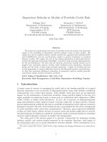
determined by the tail of the mixing distribution G(q). In Figure 1 we plot the tail function
of the probit-normal mixing model, the logit-normal model, the beta-model and the mixing
model corresponding to the Clayton copula (see Example 4.14 below) on a logarithmic sc ale.
Inspection of Figure 1 shows that the distributions diverge only after the 99% quantile, the
logit-normal m ixing-distributions being the one with the heaviest tail. From a practical
point of view this means that the particular parametric form of the mixing distribution in a
Bernoulli-mixture model is of minor importance once π and ρ
Y
have been fixed. Of course
the estimation of these parameters is a difficult task, and we will discuss several approaches
in Section 5 below.
4.3 Relation to latent variable models
At a first glance latent variable models and Bernoulli mixture models app ear to be very
different types of models. However, as has already been observed by Gordy (2000) for the
special c ase of CreditMetrics and CreditRisk
+
, these differences are often related more to
presentation and interpretation than to mathematical substance. In this section we provide
a fairly general result linking latent variable models and mixture models. Results on the
relationship between latent variable models and mixture models are useful from a theoretical
and an applied perspective. From a theoretical viewpoint results on the connection between
these model classes help to distinguish essential from inessential features of credit risk models;

from a practical point of view a link be tween the different types of models enables us to apply
numerical and statistical techniques for s olving and calibrating the models, which are natural
in the context of mixture models, also to latent variable models and vice versa. We will make
frequent use of this in Section 5.
The following condition ensures that a latent variable model can be written as a Bernoulli
mixture model.
Definition 4.9. A latent-variable-vector X has a p-dimensional conditional independence
structure with conditioning variable Ψ, if there is some p < m and a p-dimensional random
vector Ψ = (Ψ
1
, . . . , Ψ
p
)

such that conditional on Ψ the random variables (X
i
)
1≤i≤m
are
independent.
Proposition 4.10. Consider an m-dimensional latent variable vector X and a p-dimensional
(p < m) random vector Ψ. Then the following are equivalent.
(i) X has p-dimensional conditional indepen dence structure with conditioning variable Ψ.
12
B
q
P(Q>q)
0.0 0.1 0.2 0.3
10^−6 10^−5 10^−4 10^−3 10^−2 10^−1 10^0
Probit−normal

Beta
Logit−normal
Clayton
Figure 1: Tail of the mixing distribution G of Q in four different exchangeable
Bernoulli mixture models: beta (close to one-factor CreditRisk
+
); probit-normal (one-factor
KMV/CreditMetrics); logit-normal (CreditPortfolioView); Clayton. In all cases the first two
moments π and π
2
have the values for group B in Table 1. Horizontal line at 0.01 shows
that models only really start to diverge around 99th percentile of mixing distribution.
13
(ii) For any choice of thresholds d
i
1
, 1 ≤ i ≤ m the default indicators Y
i
= 1
{X
i
≤d
i
1
}
follow
a Bernoulli mixture model with factor Ψ; the conditional default probabilities are given
by Q
i
(Ψ) = P (X

i
≤ d
i
1
| Ψ).
Example 4.11 (Normal mean-variance mixtures with factor structure). Suppose
that the latent variables X have a normal mean-variance mixture distribution as in Ex-
ample 3.5 so that X
i
= µ
i
(W ) + g(W)Z
i
for W independent of Z
i
. Suppose also that Z
(and hence X) follows the linear factor model (3), so that Z
i
=

p
j=1
a
i,j
Θ
j
+ σ
i
ε
i

for a ran-
dom vector Θ ∼ N
p
(0, Ω) and indepe ndent, standard normally distributed random variables
ε
1
. . . , ε
m
, which are also independent of Θ. Then X has a (p + 1)-dimensional conditional
independence structure.
To see this define the (p + 1)-dimensional random vector Ψ by Ψ = (Θ
1
, . . . , Θ
p
, W )

and observe that conditional on Ψ the random variables X
i
are independent and normally
distributed with mean µ
i
(W ) + g(W)

p
j=1
a
ij
Θ
j
and variance (g(W )σ

i
)
2
. The equivalent
Bernoulli mixture model is now easy to compute. Given thresholds (d
i
1
)
1≤i≤m
we get condi-
tional default probabilities
Q
i
(Ψ) = P (X
i
≤ d
i
1
| Ψ) = Φ

d
i
1
− µ
i
(W ) − g(W )

p
j=1
a

ij
Θ
j
g(W )σ
i

. (18)
In the special case of multivariate t latent variables we obtain
Q
i
(Ψ) = Φ

σ
−1
i

d
i
1

W/ν −

p
j=1
a
ij
Θ
j

. (19)

The formula (18) is the key to Monte Carlo simulation for latent variable models with
normal mixture distributions in a large portfolio context. For example, rather than sim-
ulating an m-dimensional t distribution to implement the Student model, we are simply
required to simulate a p-dimensional normal vector Θ with p  m, an independent chi-
squared variate W and then to conduct a series of independent Bernoulli experiments with
default probabilities Q
i
(Ψ) to decide whether individual counterparties default.
Example 4.12 (Archimedean copulas). As shown in the following lemma, which is
essentially due to Marshall and Olkin (1988), latent variable models based on exchangeable
Archimedean copulas possess a one-dime nsional conditional independence structure. The
relevance of this result to credit risk modelling is also discussed in Sch¨onbucher (2002).
Lemma 4.13. Given a distribution function F on R
+
with Laplace transform ϕ(x) =

∞
0
exp(−xy)dF (y), and suppose that F (0) = 0. Denote by ϕ
−1
the functional inverse
of ϕ. Consider a random variable Ψ ∼ F and a sequence (U
i
)
1≤i≤m
of random vari-
ables which are conditionally independent given Ψ with conditional distribution function
P (U
i
≤ u | Ψ = ψ) = exp(−ψϕ

−1
(u)) for u ∈ [0, 1]. Then
P (U
1
≤ u
1
, . . . , U
m
≤ u
m
) = ϕ(ϕ
−1
(u
1
), . . . , ϕ
−1
(u
m
)) ,
so that (U
i
)
1≤i≤m
has an Archimedean copula with generator φ = ϕ
−1
. Moreover, every
Archimedean copula can be obtained that way.
The Lemma gives a recipe for simulating from an Archimedean copula with generator
φ. We need to find a distribution function whose Laplace transform is φ
−1

so that we can
simulate values of Ψ. In a second stage we then simulate independently variates U
i
with
distribution function F (u) = exp(−Ψφ(u)). For a list of some Archimedean copulas where
this is possible see Joe (1997) or Sch¨onbucher (2002).
Consider now a latent variable model (X
i
, d
i
1
), 1 ≤ i ≤ m where X has an exchangeable
Archimedean copula with generator φ. Put Y
i
= 1
{X
i
≤d
i
1
}
and p
i
= P (Y
i
= 1). Using
Lemma 4.13, an equivalent Bernoulli mixture model is now straightforward to compute.
14
Observe that for Ψ and U
1

. . . U
m
as in the Lemma

X
i
, d
i
1

1≤i≤m
and (U
i
, p
i
)
1≤i≤m
are
two equivalent latent variable modes by Proposition 3.2. Moreover, the U
i
are obviously
independent given Ψ and we obtain for the conditional default probabilities
P (U
i
≤ p
i
| Ψ) = Q
i
(Ψ) := exp(−Ψφ(p
i

)) .
To simulate from the Archimedean copula-based latent variable model we may therefore use
the following efficient and simple approach. In a first step we simulate a realisation of Ψ
and then we conduct m independent Bernoulli experiments with default probabilities Q
i
(Ψ)
to simulate a realisation of defaulting counterparties.
Example 4.14 (The Clayton Copula). As a concrete example again consider the Clay-
ton copula of Example 3.6 with generator φ(t) = t
−θ
− 1. Suppose we wish to construct an
exchangeable Bernoulli mixture model with default probability π and joint default probabil-
ity π
2
which is equivalent to a latent variable mo del driven by the Clayton copula. Using (4)
the required value of θ to give the desired default probabilities is the solution to the equation
π
2
= C
θ
(π, π) = (2π
−θ
− 1)
−1/θ
, θ > 0.
It is easily seen that π
2
and hence default correlation in our exchangeable Bernoulli mixture
model is increasing in θ; for θ → 0 we obtain indepe ndent defaults, for θ → ∞ defaults
become c omonotonic and default correlation tends to one. A gamma(1/θ) variate Ψ with

density g(q) = q
1/θ−1
exp(−q)/Γ(1/θ) has Laplace transform equal to the generator inverse
φ
−1
(t) = (t + 1)
−1/θ
, so that a mixing distribution on [0, 1] would be defined by setting
Q = exp(−Ψ(π
−θ
− 1)). In effect we use a mixing distribution where − log Q has a two-
parameter gamma distribution. The Bernoulli mixture model implied by the Clayton copula
will be used in Section 5.1. See also Sch¨onbucher (2002) for more discussion of the technique
used in this example.
5 Calibration of Bernoulli mixture models
In this section we consider fitting Bernoulli mixture models to historical default data. We
envisage three s ituations of increasing complexity.
• Calibration of a model for a single homogeneous group of obligors with some common
credit rating. We consider various approaches to estimating the parameters of an
exchangeable Bernoulli mixture model, in particular the default correlation.
• Calibration of a model for a large portfolio divided into a number of different rating
categories. Here we assume that rating category is the only available covariate for each
obligor and that historical default data have been collected for each rating class (either
internally or by a rating agency using a comparable rating system). We fit the model
of Example 4.4 to data collected in Standard and Poor’s (2001).
• Calibration of a latent variable model where the latent variables have a normal variance
mixture distribution. Here we envisage a portfolio where the default potential of
individual obligors is considered to be better understood so that they are treated more
heterogeneously. We assume that a partial calibration of the model is undertaken using
the approach of KMV/CreditMetrics but that some parameters of the latent variable

distribution remain unknown and these are to be estimated from historical data using
the equivalent Bernoulli mixture model.
15
5.1 Calibration of an exchangeable model
Suppose we have n years of data on historical default numbers for a homogeneous group;
for j = 1, . . . , n let m
j
denote the number of obligors observed in year j and let M
j
denote
the number that default. Further suppose that these defaults are generated by an exchange-
able Bernoulli mixture model so that there exist identically distributed mixing variables
Q
1
, . . . , Q
n
and defaults in year j are conditionally independent given Q
j
. We consider two
generic methods for estimating the fundamental parameters π = π
1
, π
2
and ρ
Y
: the method
of moments and the maximum likelihood method.
A natural moment-style estimator of π
k
is given by

π
k
=
1
n
n

j=1

M
j
k


m
j
k

=
1
n
n

j=1
M
j
(M
j
− 1) · · · (M
j

− k + 1)
m
j
(m
j
− 1) · · · (m
j
− k + 1)
, 1 ≤ k ≤ min{m
1
, . . . , m
n
}. (20)
To understand this estimator observe that

M
j
k

represents the number of possible subgroups
of k obligors among the defaulting obligors in year j. If we write Y
j,1
, . . . , Y
j,m
j
for the default
indicators of the obligors oberved in year j we have

M
j

k

=

i
1
, ,i
k
: {i
1
, ,i
k
}⊂{1, ,m
j
}
Y
j,i
1
· · · Y
j,i
k
,
so that E(

M
j
k

/


m
j
k

) = π
k
follows by taking expectations of both sides. We estimate the
unknown theoretical moment π
k
by taking the natural empirical average (20) constructed
from the n years of data. The estimator is unbiased for π
k
and consistent (as n → ∞);
for more details see Frey and McNeil (2001). Obviously ρ
Y
can be estimated by taking
ρ
Y
= (π
2
− π
2
)/(π − π
2
).
An alternative moment-style estimator of π
2
has bee n proposed by Gordy (2000) and, in
the notation of our paper, this takes the form
π

2
= π
2
+
1
n

n
j=1

M
j
m
j
− π

2
−
π(1−π)
n

n
j=1
1
m
j
1 −
1
n


n
j=1
1
m
j
. (21)
For a derivation see Appendix B of Gordy (2000).
To implement a maximum likelihood (ML) procedure we assume a simple parametric
form for the density of the Q
j
(such as beta, logit- or probit-normal); the joint probability
function of the data is then calculated using (10) under the assumption that the Q
j
are in-
dependent and maximised with respect to the natural parameters of the mixing distribution
(i.e. a and b in the case of beta and µ and σ for the logit- and probit-normal). If inde-
pendence seems unrealistic the method can be considered as a quasi-maximum-likelihood
(QML) procedure which should still yield reasonable parameter estimates. The ML esti-
mates of π = π
1
, π
2
and ρ
Y
are calculated by evaluating moments of the fitted distribution
using (11).
To decide which of these approaches is the best way to estimate these parameters we have
conducted a simulation study (summarised in Table 2) of the performance of the moment
method using both (20) and (21) and the ML method based on the assumption of a beta
mixing distribution. Computationally the beta mixture model is the easiest of the mixture

models to fit because evaluation of the joint probability of the data can be achieved without
numerical integration; this makes it fast and easy to perform in a large simulation study.
To generate data in the simulation study we consider three different Bernoulli mixture
models: the beta and probit-normal mixing models of Section 4.1.1; the mixing model im-
plied by a latent variable model with Clayton copula as in Example 4.14. In any single
experiment we generate 20 years of data using parameter values that roughly correspond
16
Model Parameter CCC B BB
All models π 0.188 0.049 0.0112
π
2
0.042 0.00313 0.000197
ρ
Y
0.0446 0.0157 0.00643
Beta a 4.02 3.08 1.73
b 17.4 59.8 153
Probit-Normal µ -0.93 -1.71 -2.37
σ 0.316 0.264 0.272
Clayton π 0.188 0.049 0.0112
θ 0.0704 0.032 0.0247
Table 1: Parameter values used in the simulation study of Table 2. These correspond very
roughly to the CCC, B and BB rating classes of Standard and Poors.
to one of the credit ratings CCC, B or BB of Standard & Poors; see Table 1 for the pa-
rameter values. The number of firms m
j
in each of the years is generated randomly using
a binomial-beta model to give a spread of values typical of real data; the defaults are then
generated using one of the Bernoulli mixture models and the three methods are com pared.
The experiment is repeated 5000 times and a relative root mean square error (RRMSE)

is estimated for each parameter and each method; that is we take the square root of the
estimated MSE and divide by the true parameter value.
It may be concluded from Table 2 that for es timating default probabilities the standard
method (20) is good enough and gives an essentially identical performance to an approach
based on fitting a Bernoulli mixture model with beta mixing distribution. However for
estimating π
2
and ρ
Y
the ML method is (almost) alway best and outperforms the moment
estimators even in the models where the beta distribution is misspecified. This can be
explained by the fact that - as shown in Example 4.8 - when we constrain well-behaved,
unimodal mixing distributions with densities (such as our four choices) to have the same
first and second moments these distributions are very similar. Of the moment formulae for
π
2
(20) should be preferred as the better quick method of getting an e stimate . It can also be
noted that the ML method tends to outperform the moment methods more as we increase
the credit quality so that defaults become rarer.
5.2 Calibration of model for several exchangeable groups
In view of the results in Table 2 we apply a ML approach to fitting more complex models.
We now suppose that in each year we have data for k different rating classes indexed by
r = 1, . . . , k. In year j the cohort consists of m
j,r
obligors in rating class r, of which M
j,r
default in the course of the year.
It is possible to generalise the beta mixture model of the previous section to obtain a
regression model for grouped data (see Joe, page 216), but numerical integration to obtain
the model likelihood can generally not be avoided in realistic models and we find it equally

convenient to switch to the probit-normal (or logit-normal) mixing distribution and fit the
model of Example 4.4. Thus we assume that in year j the conditional distribution of M
j
=
(M
j,1
, . . . , M
j,k
)

is of the form (14) given a standard normally distributed factor variable
Ψ
j
, and the unconditional probability function is obtained by integrating over this factor.
To complete the specification we assume that the factor random variables Ψ
1
, . . . , Ψ
n
for
each of the different years are iid standard normal. Again this may be considered to be a
QML approach if the assumption of independent factor variables seems unrealistic. We also
assume that for j
1
= j
2
, M
j
1
and M
j

2
are conditionally independent given Ψ
j
1
and Ψ
j
2
.
Thus the joint distribution of M
1
, . . . , M
n
is the product of the marginal distributions of
17
Group True Model Par. MomentA MomentB MLEbeta
RRMSE ∆ RRMSE ∆ RRMSE ∆
CCC beta π 0.101 0 0.101 0 0.101 0
CCC beta π
2
0.202 0 0.204 1 0.201 0
CCC beta ρ
Y
0.332 5 0.344 9 0.317 0
CCC clayton π 0.102 0 0.102 0 0.102 0
CCC clayton π
2
0.205 1 0.207 2 0.204 0
CCC clayton ρ
Y
0.331 8 0.344 12 0.306 0

CCC probitnorm π 0.100 0 0.100 0 0.100 0
CCC probitnorm π
2
0.205 1 0.208 2 0.204 0
CCC probitnorm ρ
Y
0.347 11 0.361 15 0.314 0
B beta π 0.130 0 0.130 0 0.130 0
B beta π
2
0.270 0 0.275 2 0.269 0
B beta ρ
Y
0.396 8 0.409 12 0.367 0
B clayton π 0.134 0 0.134 0 0.133 0
B clayton π
2
0.293 3 0.299 5 0.284 0
B clayton ρ
Y
0.432 17 0.449 22 0.368 0
B probitnorm π 0.130 0 0.130 0 0.130 0
B probitnorm π
2
0.286 3 0.292 5 0.277 0
B probitnorm ρ
Y
0.434 19 0.451 24 0.364 0
BB beta π 0.199 0 0.199 0 0.199 0
BB beta π

2
0.435 0 0.447 3 0.438 1
BB beta ρ
Y
0.508 7 0.526 10 0.476 0
BB clayton π 0.196 0 0.196 0 0.195 0
BB clayton π
2
0.475 8 0.490 12 0.438 0
BB clayton ρ
Y
0.588 22 0.610 27 0.480 0
BB probitnorm π 0.197 0 0.197 0 0.197 0
BB probitnorm π
2
0.492 10 0.509 14 0.446 0
BB probitnorm ρ
Y
0.607 27 0.631 31 0.480 0
Table 2: Each panel of the table relates to a block of 5000 simulations using a particular
exchangeable Bernoulli mixture model with parameter values roughly corresponding to a
particular S&P rating class. For each parameter of interest an e stimate d RRMSE (relative
root MSE) is tabulated for each of the three estimation methods: moment estimation based
on (20) denoted MomentA; moment estimation based on (21) denoted MomentB; ML esti-
mation based on the beta model. Methods can be compared by using ∆ - the percentage
inflation of the estimated RRMSE with respect to the best method (i.e. the RRMSE min-
imising method) for each parameter. Thus for each parameter the best method has ∆ = 0.
The table clearly shows that MLE performs (almost) always best.
18
the M

j
and the log-likelihood takes the form
L(µ, σ; M
1
, . . . , M
n
) =
n

j=1
k

r=1
log

m
j,r
M
j,r

+
n

j=1
log I
j
where µ = (µ
1
, . . . , µ
k

)

and σ = (σ
1
, . . . , σ
k
)

are the unknown model parameters and
I
j
=

∞
−∞
k

r=1
(h(µ
r
+ σ
r
z))
M
j,r
(1 − h(µ
r
+ σ
r
z))

m
j,r
−M
j,r
φ(z)dz.
Maximisation of the log-likelihood with respect to µ and σ requires n numerical integrations
for every point at which the log-likelihood is evaluated. To avoid numerical problems we
have found it useful to make the substitution q = Φ(z) and to rewrite and evaluate I
j
as
I
j
=

1
0
exp

k

r=1
M
j,k
log

h(µ
r
+ σ
r
Φ

−1
(q))

+ (m
j,r
− M
j,r
) log

1 − h(µ
r
+ σ
r
Φ
−1
(q))


dq.
Having obtained estimates of

µ and

σ, we can easily infer estimates of default probabil-
ities as well as within-group and between-group default correlations for each of the groups.
We use (13) to calculate estimates
π
(r)
:=


∞
−∞
h(µ
r
+ σ
r
z)φ(z)dz, 1 ≤ r ≤ k
π
(r,s)
2
:=

1
0

h(µ
r
+ σ
r
Φ
−1
(q))h(µ
s
+ σ
s
Φ
−1
(q))

dq, 1 ≤ r, s ≤ k,

where π
(r,s)
2
gives the estimated default probability for a pairs of obligors chosen respectively
from groups r and s. The matrix of estimated within-group and between-group default
correlations has (r, s)-element given by
ρ
(r,s)
Y
=
π
(r,s)
2
− π
(r)
π
(s)

(π
(r)
− π
(r)2
)(π
(s)
− π
(s)2
)
,
where the diagonal elements ρ
(r,r)

Y
are the estimated within-group default correlations.
Example 5.1 (Standard and Poor’s Data). In Standard and Poor’s (2001) (see Table 13
on pages 18-21) one-year default rates for groups of obligors formed into cohorts (described
as static pools) in the years 1981-2000 can be found. From this information it is possible to
infer the actual numbers of defaulting obligors. Standard and Poor’s use the ratings AAA,
AA, A, BBB, BB, B, CCC, but because the one-year default rates for AAA and AA-rates
obligors are largely zero, we concentrate on the rating categories A to CCC where defaults
over the one-year horizon are observed. Thus we work with n = 20 years of data and k = 5
rating classes.
The parameter estimates obtained by maximum likelihood in the case of the probit
link function are given in Table 3, together with the estimated default probabilities π
(r)
and estimated default correlations ρ
(r,s)
Y
that these imply. These values may prove a useful
reference for researchers who seek plausible values for default correlations and probabilities
in other studies of portfolio credit risk. Note that these default correlations are correlations
between event indicators for very low probability events and are necessarily very small.
The fitted model summarised in Table 3 can be used in conjunction with (17) to give
large sample risk measure estimates. The steps required are as follows.
1. The portfolio is mapped to the S&P rating system. For example, consider a low-grade
portfolio of 10000 obligors where the numbers of A, BBB, BB, B and CCC-rated firms
are 2000, 1000, 1000, 3000, 3000.
19
Parameter A BBB BB B C
µ
r
-3.40 -2.90 -2.41 -1.69 -0.84

s.e.(µ
r
) 0.14 0.09 0.08 0.06 0.08
σ
r
0.189 0.205 0.252 0.239 0.262
s.e.(σ
r
) 0.17 0.10 0.07 0.05 0.07
π
(r)
0.004 0.0022 0.0098 0.0503 0.2066
ρ
(r,s)
Y
A BBB BB B C
A 0.00022 0.00047 0.00103 0.00166 0.00256
BBB 0.00047 0.00103 0.00223 0.00361 0.00564
BB 0.00103 0.00223 0.00484 0.00791 0.01226
B 0.00166 0.00361 0.00791 0.01303 0.02048
C 0.00256 0.00564 0.01226 0.02048 0.03270
Table 3: Maximum likelihood parameter estimates and standard errors for a one-factor Bernoulli
mixture model fitted to historical Standard and Poor’s one-year default data, together with the
implied estimates of default probabilities π
(r)
and default correlations ρ
(r,s)
Y
that these imply. Note
that we have tabulated default c orrelation in absolute terms and not in percentage terms.

2. The inputs to formula (17) are determined. In our case we have m = 10000, k = 5,
λ
1
= 0.2, λ
2
= 0.1, λ
3
= 0.1, λ
4
= 0.3, λ
5
= 0.3. The parameters µ
1
, . . . , µ
5
, σ
1
, . . . , σ
5
are replaced by the estimates in Table 3. The h function is the probit link function
h(x) = Φ(x), wher Φ is the standard normal distribution function.
3. For typical values of α, such as 99% or 99.9% the formula is evaluated to give estimates
of the corresponding credit portfolio VaR. In our e xample we get q
0.99
(L
(10000)
) ≈ 1652
and q
0.999
(L

(10000)
) ≈ 2039.
The implied default probability and default correlation estimates in Table 3 could be used
to calibrate stochastic models other than the probit-normal model to the S&P default data.
For example, to calibrate a Clayton copula to group BB we use the inputs π
(3)
= 0.0098 and
ρ
(3,3)
Y
= 0.00484 to determine the parameter θ of the Clayton copula.
5.3 Calibration of normal variance mixtures
We now turn our attention to the calibration of models for m ore heterogeneous groups of
obligors constructed using the latent variable philosophy underlying KMV and CreditMet-
rics. We assume the factor structure of the latent variables X has dimension greater than
one and the dispersion matrix Σ of the latent variables has rich structure. This renders the
approach of trying to statistically estimate all parameters of an equivalent mixture model
from historical default data practically impossible, since relevant data for many parameters
will be scarce.
Under these circumstances other approaches to model calibration are used. Default
probabilities are either inferred using internal or external ratings or, via variants of the
Merton (1974) model from equity values. The parameters describing the factor model are
chosen either by an ad-hoc consideration of which factors influence asset returns and to what
extent, or possibly by a more formal regression analysis of asset returns (or a proxy like equity
returns) against economic factors. In the spirit of this approach we will as sume then that
individual default probabilities and the factor structure of X as summarised by the matrix
Σ are given.
1
For a Gaussian latent variable model this completes the calibration but, as we
have seen in Example 3.5, it is possible to develop latent variable models with non-Gaussian

1
Note that this is exactly the information which is provided by the KMV-Moodys model to subscribers of
the service.
20
distribution and more parameters. In this section we will consider how the calibration of a
model with multivariate t-distributed latent variables could b e completed by estimating the
degrees of freedom parameter ν; thus we obtain a hybrid calibration method which combines
a rational calibration based on consideration of relevant economic factors affecting default
as well as an adjustment to improve the fit of the model to observed historical defaults. The
approach would extend to other normal mean-variance mixture models with more unknown
parameters in the mixing distribution.
As before let m
j
, 1 ≤ j ≤ n be the number of obligors in the sample of observed firms in
year j. In any given year the default indicator vector Y
j
= (Y
j,1
, . . . , Y
j,m
j
)

is induced by a
latent variable model (X
j,i
, d
j,i
1
), 1 ≤ i ≤ m

j
, where the latent variable vector X
j
follows a
multivariate t distribution with factor structure. The conditional default probability of the
ith obligor in year j follows from (19) and is given by
P (Y
j,i
= 1 | Θ
j
= θ, W
j
= w) = Q
j,i
(θ, w) := Φ

d
j,i
1

w/ν − (A
j
θ)
i
σ
j,i

, (22)
where in every year j the matrix A
j

(determining the factor structure) and the constants
d
j,i
1
and σ
j,i
(determining the individual default probabilities) are considered known. Fur-
thermore we assume that W
j
is independent of Θ
j
for all j and that (W
j
, Θ
j
)
1≤j≤n
forms
an iid sequence of random vectors.
To complete the model fitting we use ML estimation to determine the parameter ν of the
chi-squared distribution of the W
j
. Denote by y
j
= (y
j,1
, . . . , y
j,m
j
)


the default-observations
in year j. Let B
j
= {1 ≤ i ≤ m
j
: y
j,i
= 1} be the identities of the firms which have
defaulted in year j, and B
c
j
:= {1, . . . , m
j
} − B
j
the identities of the surviving firms. Using
the conditional independence of the default indicators we obtain
P (Y
j
= y
j
| W
j
, Θ
j
) =

i∈B
j

P (Y
j,i
= 1 | Θ
j
, W
j
)

i∈B
c
j
(1 − P(Y
j,i
= 1 | Θ
j
, W
j
)) . (23)
The unconditional default probability function of the observations depends on the unknown
parameter ν and is given by
P (Y
j
= y
j
; ν) =

R

R
p

P (Y
j
= y
j
| Θ
j
= θ, W
j
= w)dF
0,Ω
j
(θ)dG
ν
(w) ,
where F
0,Ω
j
(θ) denotes the joint distribution function of a N
p
(0, Ω
j
)-distributed random
vector and G
ν
denotes the distribution function of a χ
2
ν
random variable. Under our inde-
pendence assumptions the log-likelihood function for given observations y
1

, . . . , y
n
equals
L(ν; y
1
, . . . , y
n
) =

n
j=1
ln P (Y
j
= y
j
; ν) , and this is maximised with respect to ν.
The main practical obstacle is the evaluation of the double integral in the log-likelihood
and the approach that we use is Monte Carlo simulation. We make the following practical
observations about the method. First, although the likelihood contribution (23) assumes
that every obligor is completely heterogeneous it is advisable to group obligors as far as
possible into homogeneous groups with identical default probabilities and factor structure.
The main advantage of this approach is better numerical performance of the MC-simulation
in the computation of the log-likelihood function. Second, it is very useful to use multivariate
importance sampling. Since the approach is useful for working with normal mixture models
in general, we briefly sketch the idea.
To compute the expectation E(f (X)), where X = g(W )Z follows a normal mixture
model with Z ∼ N(0, Σ) and Σ = AA

, we use the identity
E(f(X)) =


R

R
d
f(g(w)A
˜
z) dF
0,I
(
˜
z) dG(w)
=

R

R
d
dF
0,I
(
˜
z)
dF
µ(w),I
(
˜
z)
f(g(w)A
˜

z) dF
µ(w),I
(
˜
z) dG(w) .
21

probability
60 80 100 120
0.0 0.01 0.02 0.03
Figure 2: Density plot of estimates of the 99% quantile of M, the number of defaults, in a latent vari-
able model with t distributed latent variables and factor structure. The true value is approximately
equal to 80. Details are given in Section 5.3.
The new mean µ(w) of the relocated multivariate normal distribution with distribution
function F
µ(w),I
, which may depend on the realization w of the mixing variable W , is chosen
so that the second moment of the inner integral is reduced. This can be done using standard
importance sampling techniques for multivariate normal random variables; in particular the
density ratio dF
0,I
/dF
µ(w),I
is easily computed.
Example 5.2 (A simulation Experiment). To assess the feasibility of the above approach
in real applications we constructed a hypothetical situation using simulated data. We as-
sumed the availability of 20 years of data and considered a test portfolio of 400 obligors
belonging to three homogeneous groups with different exposures to two systematic factors.
The latent variables governing default were assumed to have a t distribution with 10 degrees
of freedom. K = 100 random datasets of 20-year default patterns were generated and ν was

estimated from each dataset using the MC approach to evaluating the likeliho od.
For each estimate ν
k
, k = 1, . . . , K we evaluated q
0.99
(M; ν
k
), the approximate 99%
quantile of the distribution of defaults implied by (16). Since the tail of the loss distribution
is the key object of interest in credit portfolio management, a density plot of the estimated
values q
0.99
(M; ˆν
k
), k = 1, . . . , K as in Figure 2 permits a good assessment of the performance
of the estimator. The true value in our simulated model is q
0.99
(M; 10) ≈ 80 and in a
Gaussian model it would be q
0.99
(M; ∞) ≈ 58. Since our estimates are concentrated around
80 it appears that the estimator is mostly able to distinguish the riskier t model with ν = 10
from a normal model.
2
This suggests that in the context of a normal variance mixture
models ML estimation might be useful in reducing the model risk related to the choice of
the copula.
2
Theoretically q
0.99

(M; ∞) is a lower bound for the distribution of q
0.99
(M; ˆν); the mass below 58 in
Figure 2 is due to the kernel-estimator used in the density plot.
22
6 Conclusion
Ultimately, the goal of academic research on credit risk models is to help the practitioner in
specifying a model, which is appropriate for his or her lending portfolio. We therefore con-
clude with a few recommendations on model choice, which summarise the practical aspects
of our research.
Bernoulli mixture m odels are more convenient than latent variable models when it comes
to both estimation and simulation, at least for large portfolios. If one prefers to work with a
latent variable model, the model should have a conditional independence structure, so that
it admits an equivalent representation as a mixture model. As we have shown in Section 4.3,
there is a wide range of latent variable models with this property.
One-factor regression models such as the model considered in Example 4.4 are reasonable
models for portfolios with a relatively homogeneous exposure to a common set of risk factors.
They are also useful parsimonious models in a situation where we have only rather imprecise
information on the risk factors affecting a portfolio, s uch that we have to rely solely on
historical default information in estimating model parameters. As we have seen in Section 5.1
and Section 5.2, maximum likelihoo d fitting of Bernoulli mixture models is a feasible method
of obtaining estimates of model parameters and the precise choice of the mixing distribution
is of lesser importance. Moreover, maximum likelihood methods seem to perform better
than simple moment estimation techniques. We further note that the models we have fitted
essentially belong to the class of generalised linear mixed models (GLMMs); although we
have taken a maximum likelihood approach it would also be possible to use computational
Bayesian methods such as Markov Chain Monte Carlo to fit such models.
For a portfolio, where obligors are exposed to several risk factors and where the exposure
to different risk factors differs markedly across obligors, such as a portfolio of loans to larger
corporations active in different industries or countries, we recommend a normal variance

mixture model with factor structure. Calibration of the factor structure can be done by an
analysis of asset returns or a proxy such as equity returns; the parameters of the mixing
distribution can be estimated from historical default data using the approach developed in
Section 5.3.
References
Credit-Suisse-Financial-Products (1997): “Cre ditRisk
+
a Credit Risk Management
Framework,” Technical Document, available from htpp://www.csfb.com/creditrisk.
Crosbie, P., and J. Bohn (2002): “Modeling default risk,” KMV working paper, available
from .
Crouhy, M., D. Galai, and R. Mark (2000): “A comparative analysis of current credit
risk models,” Journal of Banking and Finance, 24, 59–117.
Davis, M., and V. Lo (2001): “Infectious defaults,” Quantitative Finance, 1, 382–387.
Duffie, D., and K. Singleton (1999): “Modeling Term Structure Models of Defaultable
Bonds,” Review of Financial Studies, 12, 687–720.
Eberlein, E., and U. Keller (1995): “Hyperbolic Distributions in Finance,” Bernoulli,
1, 281–299.
Embrechts, P., A. McNeil, and D. Straumann (2001): “Correlation and dependency
in risk management: prop erties and pitfalls,” in Risk Management: Value at Risk and
Beyond, ed. by M. Dempster, and H. Moffatt. Cambridge University Press.
23
Frey, R., and A. McNeil (2001): “Modelling dependent defaults,” ETH E-Collection,
URL ETH Z¨urich.
Frey, R., and A. McNeil (2002): “VaR and Expected Shortfall in Portfolios of Dependent
Credit Risks: Conceptual and Practical Insights,” Journal of Banking and Finance, pp.
1317–1344.
Frey, R., A. McNeil, and N. Nyfeler (2001): “Copulas and Credit Models,”
RISK,14(October) pp. 111–114.
Giesecke, K. (2001): “Structural modelling of defaults with incomplete information,”

preprint, Humboldt-Universit¨at Berlin, forthcoming in Journal of Banking and Finance.
Gordy, M. (2000): “A comparative anatomy of credit risk models,” Journal of Banking
and Finance, 24, 119–149.
Gordy, M. (2001): “A Risk-Factor model foundation for ratings-based capital rules,” work-
ing paper, Board of Governors of the Federal Reserve System, forthcoming in Journal of
Financial Intermediation.
Jarrow, R., and F. Yu (2001): “Counterparty risk and the pricing of defaultable securi-
ties,” Journal of Finance, 53, 2225–2243.
Joe, H. (1997): Multivariate Models and Dependence Concepts. Chapman & Hall, London.
Kealhofer, S., and J. Bohn (2001): “Portfolio management of default risk,” KMV work-
ing paper, available from .
Koyluoglu, U., and A. Hickman (1998): “Reconciling the Differences,” RISK, 11(10),
56–62.
Lando, D. (1998): “Cox processes and credit risky securities,” Review of Derivatives Re-
search, 2, 99–120.
Li, D. (2001): “On default correlation: a Copula function approach,” Journal of Fixed
Income, 9, 43–54.
Lindskog, F. (2000): “Modelling Dependence with Copulas,” RiskLab Report, ETH
Zurich.
Marshall, A., and I. Olkin (1988): “Families of multivariate distributions,” Journal of
the American Statistical Assosiation, 83, 834–841.
Merton, R. (1974): “On the Pricing of Corporate Debt: The Risk Structure of Interest
Rates,” Journal of Finance, 29, 449–470.
Nelsen, R. B. (1999): An Introduction to Copulas. Springer, New York.
Petrov, V. V. (1975): Sums of Independent Random Variables. Springer, Berlin.
RiskMetrics-Group (1997): “CreditMetrics – Technical Doc ument,” available from
/>Sch
¨
onbucher, P., and D. Schubert (2001): “Copula-dependent default risk in intensity
models,” preprint, Universit¨at Bonn.

Sch
¨
onbucher, P. J. (2002): “Taken to the limit,” Preprint, Universit¨at Bonn.
Schweizer, B., and A. Sklar (1983): Probabilistic Metric Spaces. North–
Holland/Elsevier, New York.
24
Standard, and Poor’s (2001): “Ratings Performance 2000: Default, Transition, Recovery,
and Spreads,” .
Wilson, T. (1997): “Portfolio Credit Risk I and II,” RISK, 10(Sept and Oct).
A Copulas
In the following we present a brief introduction to copulas. For further reading see Em-
brechts, McNeil, and Straumann (2001), Joe (1997) and Nelsen (1999).
Definition A.1 (Copula). A copula is a multivariate distribution with standard uniform
marginal distributions, or the distribution function of such a distribution.
We use the notation C(u) = C(u
1
, . . . , u
d
) for the d-dimensional joint distribution func-
tions which are copulas. C is a mapping of the form C : [0, 1]
d
→ [0, 1], i.e. a mapping of the
unit hypercube into the unit interval. The following three properties characterise a copula
C.
1. C(u
1
, . . . , u
d
) is increasing in each component u
i

.
2. C(1, . . . , 1, u
i
, 1, . . . , 1) = u
i
for all i ∈ {1, . . . , d}, u
i
∈ [0, 1].
3. For all (a
1
, . . . , a
d
), (b
1
, . . . , b
d
) ∈ [0, 1]
d
with a
i
≤ b
i
we have:
2

i
1
=1
· · ·
2


i
d
=1
(−1)
i
1
+···+i
d
C(u
1i
1
, . . . , u
di
d
) ≥ 0,
where u
j1
= a
j
and u
j2
= b
j
for all j ∈ {1, . . . , d}.
Suppose the random vector X = (X
1
, . . . , X
d
)


has a joint distribution F with continuous
marginal distributions F
1
, . . . , F
d
. If we apply the appropriate probability transform to each
component we obtain a transformed vector (F
1
(X
1
), . . . , F
d
(X
d
)) whose distribution function
is by definition a copula, which we denote C. It follows that
F (x
1
, . . . , x
n
) = P (F
1
(X
1
) ≤ F
1
(x
1
), . . . , F

d
(X
d
) ≤ F
d
(x
d
))
= C(F
1
(x
1
), . . . , F
d
(x
d
)), (24)
or alternatively C(u
1
, . . . , u
n
) = F (F
←
1
(u
1
), . . . , F
←
d
(u

d
)), where F
←
i
denotes the generalised
inverse of the distribution function F
i
. Formula (24) shows how marginal distributions are
coupled together by a copula to form the joint distribution and is the essence of Sklar’s
theorem.
Theorem A.2 (Sklar’s Theorem). Let F be a joint distribution function with margins
F
1
, . . . , F
d
. Then there exists a copula C : [0, 1]
d
→ [0, 1] such that for all x
1
, . . . , x
d
in
R = [−∞, ∞] (24) holds; C is unique if F
1
, . . . , F
d
are continuous. Conversely, if C is a
copula and F
1
, . . . , F

d
are distribution functions, then the function F given by (24) is a joint
distribution function with margins F
1
, . . . , F
d
.
For a proof we refer to Schweizer and Sklar (1983). If F is a joint distribution function
with marginals F
1
, . . . , F
d
and (24) holds, we say that C a copula of F (or of a random
vector X ∼ F ).
A useful property of the copula of a distribution is its invariance under strictly increasing
transformations of the marginals. Let (X
1
, . . . , X
d
) be a vector of continuously distributed
risks with copula C and let T
1
, . . . , T
d
be strictly increasing functions. Then it is easily seen
that (T
1
(X
1
), . . . , T

d
(X
d
)) also has copula C.
25