Insurance-Based Credit Scores: Impact on Minority and Low Income Populations in Missouri doc
Bạn đang xem bản rút gọn của tài liệu. Xem và tải ngay bản đầy đủ của tài liệu tại đây (2.12 MB, 53 trang )
Insurance-Based Credit Scores: Impact on Minority and
Low Income Populations in Missouri
Brent Kabler, Ph.D.
Research Supervisor
Statistics Section
January 2004
Table of Contents
Description Page
Number
Abstract 1
Executive Summary 4
Introduction, Methodology, and Limitations of Study 13
Area Demographics and Credit Scores 19
Individual Characteristics and Credit Scores 30
Conclusion 38
Methodological Appendix 39
Sources 49
Charts and Figures
Description Page
Number
Table 1: Mean Credit Score by Minority Concentration 20
Table 2: % of Exposures in Worst Score Intervals by Minority Concentration 21
Table 3: Mean Credit Score by Per Capita Income 22
Table 4: % of Exposures in Worst Score Intervals by Per Capita Income 22
Table 5: Credit score, race / ethnicity, and socio-economic status 24
Table 6: % of Individuals in Worst Credit Score Interval(s), by Minority Status
and Family Income: Summary
31
Table 7: % of Individuals in Worst Credit Score Interval(s), by Minority Status
and Family Income: Company Results
32
Abstract and Overview
The widespread use of credit scores to underwrite and price automobile and
homeowners insurance has generated considerable concern that the practice may
significantly restrict the availability of affordable insurance products to minority and low-
income consumers. However, no existing studies have effectively examined whether credit
scores have a disproportionate negative impact on minorities or other demographic groups,
primarily because of the lack of public access to appropriate data.
This study examines credit score data aggregated at the ZIP Code level collected
from the highest volume automobile and homeowners insurance writers in Missouri.
Findings—consistent across all companies and every statistical test—indicate that credit
scores are significantly correlated with minority status and income, as well as a host of other
socio-economic characteristics, the most prominent of which are age, marital status and
educational attainment.
While the magnitude of differences in credit scores was very substantial, the impact
of credit scores on pricing and availability varies among companies and is not directly
examined in this study. The impact of scores on premium levels will be directly addressed in
studies expected to be completed by late 2004.
Missouri statue prohibits sole reliance on credit scoring to determine whether to
issue a policy. However, there are no limits on price increases that can be imposed due to
credit scores, so long as such increases can be actuarially justified.
This study finds that:
1. The insurance credit-scoring system produces significantly worse scores for
residents of high-minority ZIP Codes. The average credit score rank
1
in “all minority”
areas stood at 18.4 (of a possible 100) compared to 57.3 in “no minority” neighborhoods – a
gap of 38.9 points. This study also examined the percentage of minority and white
policyholders in the lower three quintiles of credit score ranges; minorities were
overrepresented in this worst credit score group by 26.2 percentage points. Estimates of
credit scores at minority concentration levels other than 0 and 100 percent are found on
page 8.
2. The insurance credit-scoring systems produces significantly worse scores for
residents of low-income ZIP Code. The gap in average credit scores between
communities with $10,953 and $25,924 in per capita income (representing the poorest and
1
Results are presented here as ranks, or more accurately, percentiles. Because of significant differences in the
scoring methods of insurers, many of the results in this report are presented as percentiles rather than as percentage
differences in the raw credit scores. Anyone who has taken a standardized test should be familiar with the term.
Scores for each company in the sample are ranked, and each raw score is then translated according to its
relative position within the overall distribution. For example, a score ranked at the 75
th
percentile means that
the score is among the top one-fourth of scores, and that 75 percent of recorded scores are worse. If the
average for non-minorities was at the 30
th
percentile, and the minority average at the 70
th
percentile, the
percentile difference is 40 percentiles. The percentile difference, calculated from the statistical models, is used herein as
a convenient way to summarize results for the non-technical reader.
1
wealthiest 5 percent of communities) was 12.8 percentiles. Policyholders in low-income
communities were overrepresented in the worst credit score group by 7.4 percentage points
compared to higher income neighborhoods. Estimates of credit scores at additional levels of
per capita income are found on page 9.
3. The relationship between minority concentration in a ZIP Code and credit scores
remained after eliminating a broad array of socioeconomic variables, such as income,
educational attainment, marital status and unemployment rates, as possible causes.
Indeed, minority concentration proved to be the single most reliable predictor of credit
scores.
4. Minority and low-income
individuals
were significantly more likely to have worse
credit scores than wealthier individuals and non-minorities. The average gap between
minorities and non-minorities with poor scores was 28.9 percentage points. The gap between
individuals whose family income was below the statewide median versus those with family
incomes above the median was 29.2 percentage points.
The following maps indicate the areas in Missouri that are most negatively affected
by the use of credit scores.
2
Lower Income Areas of Missouri Most Affected by Credit Scoring
Inset: Kansas City Region Inset: St. Louis Region
Bottom Quartile = 253 Zip Codes (out of 1,015), with 562,453 persons,
($6,153 - $13,335) or 10% of 5.6 million Missourians
Second Quartile = 254 ZIP Codes with 839,281 persons, or 15% of 5.6
($13,336-$15,326) million Missourians
3
Areas of Missouri With High Minority Concentration
Most Affected by Credit Scoring
Kansas City Region St. Louis Region
Southeast Missouri Region
%
M
i
n
o
r
i
t
y
L
e
s
s
t
h
a
n
2
0
%
2
0
%
t
o
5
0
%
O
v
e
r
5
0
%
Missourians in High-Minority ZIP codes
% Minority White, Non-
Hispanic
African-
Americans and
Hispanics
Other Total
20% to 50% 337,631 165,441 11,953 515,025
Over 50% 134,541 397,430 10,817 542,788
Total Missouri
Population
4,687,837 815,325 92,049 5,595,211
4
Executive Summary
The use of individuals’ credit histories to predict the risk of future loss has become a
common practice among automobile and homeowners insurers. The practice has proven to
be controversial not only because of concerns about how reliably credit scores may predict
risk. Many industry professionals, policymakers, and consumer groups have expressed
concern that the practice may pose a significant barrier to economically vulnerable segments
of the population in obtaining affordable automobile and homeowners coverage.
This study finds evidence that justifies such concerns.
Four questions are addressed in the study:
1. Is there a correlation between place of residence and insurance-based credit scores (called
“credit scores” or “scores” throughout the remainder of this report)? Specifically, do
residents of areas with high minority concentrations have worse average scores?
2. Do residents of poorer communities have worse average scores?
3. If credit scoring has a disproportionate impact on residents of communities with high
minority concentrations, what other socioeconomic factors might account for this fact?
4. Do minorities and poorer individuals tend to have worse scores than others, irrespective
of place of residence?
For this report, the category ‘minority’ includes all Missourians who identified
themselves as African-American or Hispanic in the 2000 census. A separate analysis of
African-Americans resulted in no substantive difference from the results presented here.
Data
Credit score data was solicited from the 20 largest automobile and homeowners
writers in Missouri for the period 1999-2001. Of these, 12—individually or combined with
sister companies—had used a single credit scoring product for a sufficient period of time to
generate a credible sample. In some instances, a single company is displayed as two separate
“companies” representing separate analyses of automobile and homeowners coverage. In
other instances, sister companies were combined to yield a more statistically credible sample.
The net result of these combinations is the 12 “companies” presented in the report.
5
Companies That Submitted Data for this Report
NAIC
Code Name
16322 Progressive Halcyon Insurance Co.
17230 Allstate Property & Casualty Insurance Co.
19240 Allstate Indemnity Co.
21628 Farmers Insurance Co., Inc.
21660 Fire Insurance Exchange
21687 Mid-Century Insurance Co.
22063 Government Employees Insurance Co.
25143 State Farm Fire And Casualty Co.
25178 State Farm Mutual Automobile Insurance Co.
27235 Auto Club Family Insurance Co.
35582 Government General Insurance Co.
42994 Progressive Classic Insurance Co.
Additional information about how the Missouri’s largest insurers use credit scores
can be found at the MDI web site, www.insurance.mo.gov.
The companies provided average credit scores by ZIP Code, as well as the
distribution of exposures (automobiles and homes) across five credit score intervals
representing equal numeric ranges. Both the average score and the percent of exposures in
the worst three intervals are used to assess to the degree to which race and ethnicity and
socioeconomic status are correlated with credit scores.
Because of the nature of the data, results are presented from two categorically
distinct levels of analysis:
1. Aggregate level—Inferences about residents in areas with high minority concentrations
or areas with lower incomes. This level of analysis does not purport to make inferences
about minority or lower-income individuals per se.
2. Individual level—Assessments of the likely impact of credit scores on minority individuals,
without reference to place of residence. These results make use of statistical models that are
widely employed in the social sciences, but findings are somewhat more speculative than are
the aggregate level results.
6
Findings
1. On average, residents of areas with high minority concentrations tend to have
significantly worse credit scores than individuals who reside elsewhere.
2. On average, residents of poor communities tend to have significantly worse credit
scores than those who reside elsewhere.
Given the variation in credit scoring methodologies, raw credit scores possess no
intrinsic meaning, and comparing raw scores across companies is of limited value.
Normalized or “standardized” results afford more meaningful comparisons. Averaged across
all companies, the spread in standardized scores between “no minority” and “all minority”
2
ZIP Codes was 38.9 percentiles—a very considerable gap.
3
For more than half of the
companies, the average scores of individuals residing in minority ZIP Codes fell into the
bottom one-tenth of scores (that is, at or lower than the 10
th
percentile). The average score
of individuals residing in non-minority ZIP Codes fell into the upper one-half of scores for
every company.
The last three columns of the table display percentile differences by income group.
On average, ZIP Codes with a per capita income of $25,924 (the top 5 percent of ZIP Codes)
had scores that were 12.8 percentiles higher than ZIP Codes with a per capita income of
$10,953 (the bottom 5 percent of ZIP Codes).
2
The statistical models incorporate data from all ZIP Codes to determine the overall relationship between
minority concentration and credit scores. Estimates derived from the models are presented here at the
extremes of 0 percent and 100 percent minority concentration for expository reasons (the meaning of values at
the extremes is usually more intuitive). For example, if the regression model indicated that every percentage
point increase in minority concentration is associated with a decrease in credit scores of 1.68 points, the impact
of increasing minority concentration to 100 percent would be a decline of 168 points. In reality, there are no
ZIP Codes whose residents are all minorities, though several ZIP Codes have more than 95 percent minority
concentration.
3
Percentile differences are based on normalized scores ranging from 0 to 100, and represent the rank of a score
relative to all other scores in the sample. Such percentiles are exactly analogous to those used for reporting
standardized test results. For example, a score falling in the 75
th
percentile means the score is among the top
one-fourth of scores. The numbers reported in the table below represent the percentile difference between
high and low minority ZIPs. For example, if the average score of high minority ZIP Codes was at the 20
th
percentile, and those for low minorities at the 80
th
percentile, the difference is 60 percentiles.
7
Standardized Credit Scores (Percentiles) by Minority Concentration and
Per Capita
Income in ZIP Code
Results of Weighted OLS Regression of Average Credit Score
Scores Coded So that a Lower Score is Worse
Average Score Percentile
by Minority Concentration
(on a scale of 100)
Average Score Percentile
by Per Capita Income
(on a scale of 100)
Company
4
100%
Minority
0%
Minority
Percentile
Difference
$10,953
(Poorest
5% of ZIP
Codes)
$25,924
(Wealthiest
5% of ZIP
Codes)
Difference
A
24.2 54.0 29.8 35.9 51.6 15.7
B
2.1 59.5 57.4 37.8 52.4 14.6
C
5.8 59.1 53.4 30.5 52.4 21.9
D
11.9 56.4 44.5 44.4 52.8 8.4
E
12.3 57.9 45.6 46.8 54.8 8.0
F
30.5 59.5 29.0 46.0 57.9 11.9
G
29.1 59.1 30.0 42.9 56.8 13.9
H*
22.4 56.0 33.6 45.2 52.8 7.6
I*
33.0 50.8 17.8 41.3 48.0 6.7
J
14.2 59.9 45.6 40.5 55.2 14.7
K
25.1 55.6 30.4 44.0 53.6 9.6
L
9.7 59.5 49.8 34.8 55.2 20.3
Average
(Unweighted) 18.4 57.3 38.9 40.9 53.6 12.8
*These two companies were unable to provide MDI with raw credit scores. Data thus consists of scores that have been furthered
modified based on non-credit related information prior to being used for rating / underwriting.
In addition to average credit scores by ZIP Code, the number of exposures
5
in five
equal credit score intervals was also collected; each interval represents the range of scores
divided by five.
6
The proportion of exposures in the worst three intervals was used, as a
parallel measure to average scores, to assess the association between race and income and
credit scores. On average, a 26.2 percentage point difference existed in the proportion of
exposures in the worst credit score group between “all minority” and non-minority ZIP
Codes. The corresponding gap between the wealthiest and poorest income groups was 7.4
percentage points.
Estimates for additional levels of minority concentration and per capita income are
displayed in the following four tables.
4
This report represents an analysis of credit scoring in general, and not the compliance of a specific company
with any laws, nor the degree to which a company deviated from the norm. Thus, no individual companies are
identified when displaying results.
5
One “exposure” is equal to one year of coverage for one automobile or home.
6
For clarification, credit score intervals are not quintiles where each interval represents an equal number of
exposures. Rather, each interval is an equal numeric range in credit scores, and exposures are not distributed
equally between intervals.
8
Percent of Exposures in Worst 3 Credit Score Intervals
by % Minority and
Per Capita
Income in a ZIP Code
Results of Weighted OLS Regression
Scores in Worst Group by Percent
Minority
Scores in Worst Group by
Per Capita
Income
Company 0%
Minority
100%
Minority
Difference $10,953
(Poorest
5% of ZIP
Codes)
$25,924
(Wealthiest
5% of ZIP
Codes)
Difference
A 41.4% 64.8% 23.4% 52.4% 44.4% 8.0%
B 8.9% 53.7% 44.9% 19.4% 12.5% 6.9%
C 20.5% 61.7% 41.2% 35.8% 25.1% 10.7%
D 26.7% 57.2% 30.6% 34.4% 28.2% 6.2%
E 33.7% 73.2% 39.5% 42.6% 35.9% 6.7%
F 38.9% 62.3% 23.5% 50.9% 39.5% 11.3%
G 14.5% 31.9% 17.4% 22.9% 16.2% 6.7%
H 21.7% 37.1% 15.5% 26.7% 22.9% 3.8%
I 68.3% 79.7% 11.4% 75.0% 68.0% 7.0%
J
12.1% 30.4% 18.3% 19.0% 13.8% 5.2%
K 13.2% 28.4% 15.2% 18.6% 14.2% 4.4%
L 21.8% 55.5% 33.7% 35.9% 24.1% 11.8%
Average
(Unweighted) 26.8% 53.0% 26.2% 36.1% 28.7% 7.4%
Standardized Credit Scores (Percentiles) by % Minority in a ZIP Code
Results of Weighted OLS Regression of Average Credit Score
Scores Coded So that a Lower Score is Worse
Company 0%
Minority
25%
Minority
50%
Minority
75%
Minority
90%
Minority
100%
Minority
A
54.0 46.0 38.2 30.9 26.8 24.2
B
59.5 37.1 18.4 7.2 3.6 2.1
C
59.2 41.3 24.2 13.1 8.2 5.8
D
56.4 42.9 30.5 20.1 14.9 11.9
E
57.9 44.4 31.6 20.6 15.2 12.3
F
59.5 48.0 44.8 37.5 33.0 30.5
G
59.1 48.4 43.6 36.3 31.9 29.1
H
56.0 46.8 37.8 29.8 25.1 22.4
I
50.8 46.0 41.7 37.1 34.5 33.0
J
59.9 46.8 34.1 23.0 17.4 14.2
K
55.6 47.6 39.4 31.9 27.8 25.1
L
59.5 44.0 29.8 17.9 12.5 9.7
Average 57.3 44.9 34.5 25.4 20.9 18.4
9
Percent of Exposures in Worst 3 Credit Score Intervals
by % Minority in a ZIP Code
Results of Weighted OLS Regression
Company 0%
Minority
25%
Minority
50%
Minority
75%
Minority
90%
Minority
95%
Minority
100%
Minority
A
41.4 47.2 53.1 58.9 62.4 63.6 64.8
B
8.9 20.1 31.3 42.5 49.2 51.5 53.7
C
20.5 30.8 41.1 51.4 57.6 59.6 61.7
D
26.7 34.3 42.0 49.6 54.2 55.7 57.2
E
33.7 43.6 53.5 63.3 69.2 71.2 73.2
F
38.9 44.7 50.6 56.5 60.0 61.2 62.3
G
14.5 18.9 23.2 27.6 30.2 31.0 31.9
H
21.7 25.5 29.4 33.3 35.6 36.4 37.1
I
68.3 71.2 74.0 76.9 78.6 79.2 79.7
J
12.1 16.7 21.2 25.8 28.5 29.5 30.4
K
13.2 17.0 20.8 24.6 26.9 27.6 28.4
L
21.8 30.2 38.6 47.1 52.1 53.8 55.5
Average 26.8 33.4 39.9 46.4 50.4 51.7 53.0
Standardized Credit Scores (Percentiles) by
Per Capita
Income in ZIP Code
Results of Weighted OLS Regression of Average Credit Score
Scores Coded So that a Lower Score is Worse
Company Bottom
1%
($8,642)
Quartile 1
($13,335)
Quartile 2
($15,326)
Quartile 3
($18,092)
T
op 1%
($50,536)
A
33.4 38.2 40.5 43.3 76.1
B
35.9 40.1 42.1 44.8 74.5
C
27.4 33.7 36.7 40.5 84.1
D
43.3 45.6 47.2 48.4 65.9
E
45.2 48.0 49.2 50.4 67.7
F
44.0 48.0 49.6 51.6 75.5
G
40.9 45.2 46.8 49.6 76.7
H
44.0 46.4 47.6 48.8 64.4
I
40.1 42.5 43.3 44.4 59.1
J
38.2 42.9 44.8 47.6 77.0
K
42.5 45.6 46.8 48.4 68.4
L
31.9 37.8 40.5 48.8 83.7
Average
(Unweighted) 38.9 42.8 44.6 47.2 72.8
10
Percent of Exposures in Worst Three Credit Score Intervals
by
Per Capita
Income a ZIP Code
Results of Weighted OLS Regression
Company Bottom 1%
($8,642)
Quartile 1
(13,335)
Quartile 2
(15,326)
Quartile 3
(18,092)
T
op 1%
(50,536)
A
53.6 51.1 50.1 48.6 31.6
B
20.5 18.3 17.4 16.1 1.4
C
37.4 34.1 32.6 30.7 7.9
D
35.3 33.4 32.6 31.4 18.3
E
43.6 41.5 40.6 39.4 25.1
F
52.6 49.1 47.6 45.5 21.3
G
23.9 21.8 20.9 19.7 5.4
H
27.3 26.1 25.6 24.8 16.7
I
76.1 73.9 73.0 71.7 56.8
J
19.8 18.2 17.5 16.5 5.5
K
19.3 17.9 17.3 16.5 7.2
L
37.7 34.0 32.4 30.2 5.1
A
verage
(Unweighted) 37.3 34.9 34.0 32.6 16.9
3. Credit scores are significantly correlated with minority concentration in a ZIP
Code, even after controlling for income, educational attainment, marital status,
urban residence, the unemployment rate and other socioeconomic factors.
Statistical models were used to control for—i.e., remove—the impact of
socioeconomic factors that might account for the correlation between race/ethnicity and
credit scores. The inclusion of such controls slightly weakened, but by no means eliminated
(or accounted for) the association between minority status and credit scores. Among all
such control variables, race/ethnicity proved to be the most robust single predictor of credit
scores; in most instances it had a significantly greater impact than education, marital status,
income and housing values. It was also the only variable for which a consistent correlation
was found across all companies.
Other variables found to be significantly correlated with credit scores across the
majority of companies were educational attainment, age, marital status, and urban residence.
Why scores should be correlated with minority status, even after controlling for such
broad measures of socioeconomic status, is not immediately clear. Such a result indicates
that the variable “minority concentration” contains unique characteristics not contained in
the “control” variables. For example, credit scores may reflect factors uniquely associated
11
with racial status (such as limited access to credit, for example). The results clearly call for
further study.
4. The minority status and income levels of
ndividuals
are correlated with credit
scores, regardless of place of residence.
i
Three different statistical models were used to assess differences in scores between
minority and low-income individuals, as opposed to residents of high minority or low-
income areas (not all of whom, of course, are minorities or poor). Based on the most
credible of the three models, African-American and Hispanic insureds had scores in
the worst credit score group at a rate of about 30 percentage points higher than did
other individuals (for example, where 30 percent of one group may have poor scores,
compared to 60 percent of another group). A gap of 30 percentage points also existed
between individuals earning below and above the median family income for
Missouri. Across companies, the gap for minority status ranged from 14 percent to 48
percent; and for income the gap ranged from 17 to 46 percent.
Difference in % of individuals in the worst 3 (of 5) credit score intervals
Estimates of Gary King’s Ecological Inference (EI) Model
7
Company
Minority Status
(% of minorities
with low scores
minus % of non-
minorities with low
scores)
Income
(% of lower-income
individuals with
low scores minus
% of higher-
income individuals
with low scores)
A 19.1% 27.7%
B 39.5% 16.8%
C 42.1% 46.1%
D 30.6% 22.5%
E 47.9% 28.5%
F 25.8% 35.6%
G 14.5% 21.0%
H 29.1% 32.8%
J 15.0% 26.7%
K 15.3% 26.4%
L 38.5% 37.2%
Unweighted
Average
28.9% 29.2%
7
The EI model is one of three employed in this report to make individual-level inferences. The other two are
Goodman’s Regression and the “Neighborhood” model, each of which is explained in the body of the report.
12
While considerable variation exists among the three models with respect to the
magnitude of estimates, all three consistently estimated a disproportionate impact based on
the minority status of individuals and an individual’s family income.
Because the data is composed of ZIP Code level aggregates, inferences about
individual-level characteristics are somewhat more speculative than are inferences about the
demographic characteristics of place of residence. Individual-level estimates in this report
result from three of the most widely-used statistical models for such purposes. While the model
results are not “proof” of an
individual-level
disproportionate impact, the evidence appears to be
substantial, credible and compelling.
13
I. Introduction
Use of credit scores by insurers has come into prominence within the last ten years.
A recent study found that more than 90 percent of personal lines insurers use credit scores
for rating or underwriting private automobile insurance (Conning & Co., 2001), and many
insurers also use credit scoring for homeowners coverage. Such scores are distinguished
from credit scores used in financial underwriting. While both lending and insurance scores
have many elements in common, insurance-based credit scores purport to predict the risk of
insurance loss rather than the risk of financial default.
The insurance industry has produced studies indicating that credit scores are
predictive of both loss frequency and severity for a wide variety of coverages. For example,
for private passenger automobile insurance, one study found credit scores highly predictive
of liability (both BI and PD), collision, comprehensive, uninsured motorist and medical
payment losses (Miller and Smith, 2003. See also Tillinghast-Towers Perrin, 1996;
Monaghan, 2000; and Kellison, Brockett, Shin, and Li, 2003).
This study does not examine the relationship between credit scores and the
likelihood of insurance losses. Regulators and consumer groups have expressed growing
concern that use of credit scores may restrict the availability of insurance products in
predominantly minority and low income communities, markets that already show signs of
significant affordability and access problems (Kabler, 2004).
Components common to most scoring models have been made public: high debt to
limit ratios, derogatory items such as collection actions, liens, and foreclosures, the number
of loan and credit card applications, and the number of credit accounts. Many of these items
are known to be correlated with both income and minority status. The largest study of its
kind, the Freddie Mac Consumer Credit Survey, concluded that both African-Americans and
Hispanics were significantly more likely to have derogatory items on their credit history than
were their white counterparts. Similar gaps were observed between income groups (Freddie
Mac, 1999).
Many analysts also contend that credit scores, which weigh items that signify
financial distress or limited availability of credit, are correlated with minority status.
Significant debate has continued about lending practices that restrict access to credit in
minority communities—a factor that could have a significant impact on insurance-based
credit scores. Minority communities in core urban areas also are more typically vulnerable to
economic dislocations, such as significantly elevated un- and under-employment rates, that
produce the kind of financial distress likely to be measured by credit scoring models.
Unfortunately, no rigorous studies have directly examined what, if any,
impact the growing prevalence of insurance credit scores has had on the availability
of insurance coverage in poor and minority communities.
14
The studies that have entered the public domain have been largely inconclusive or
suffer from serious methodological deficiencies. A study funded by the American Insurance
Association (AIA), an industry trade association, found no correlation between income and
credit scores (AIA, 1998). However, the AIA study appears to suffer from methodological
flaws so serious that no conclusions are warranted.
8
The Virginia Bureau of Insurance sponsored a study based on ZIP Code aggregates.
Unfortunately, the numeric results of the analysis were never publicly released. Rather, the
Bureau’s report stated that “Nothing in this analysis leads the Bureau to the conclusion that
income or race alone is a reliable predictor of credit scores, thus making the use of credit
scoring an ineffective tool for redlining”—a statement that could reasonably be made even
with a finding of a very significant disproportionate impact (Commonwealth of Virginia,
1999).
9
More recently, the Washington Department of Insurance sponsored a consumer
survey that matched demographic information obtained from telephone interviews with
credit scores (Pavelchek and Brown, 2003). While the study found a statistically significant
association between credit scores and income, the findings regarding the racial impact of
scoring were inconclusive, primarily because of the small number of minorities included in
the survey sampled from the relatively homogonous population of the state of Washington .
A literature review by the American Academy of Actuaries (2002) has also concluded
that existing studies were inconclusive with respect to the disproportionate impact issue.
This study begins filling that void.
Caveats and Limitations of Study
This study is based on ZIP Code-level credit score averages and is subject to certain
limitations. Unlike a survey of individuals, in which demographic data such as race and
income are obtained directly, this analysis makes inferences based on patterns observed in
aggregate relationships (such as average credit score in a ZIP Code). The reader is therefore
8
The study suffers from two serious flaws. First, based on conversations with the data provider, the data used
in the study is not a random sample of the population about which inferences are made. Rather, it is a
marketing sample that systematically excludes poorer individuals, renters, and individuals who had recently
relocated. Secondly, the dependent variable, income, is not directly measured but rather estimated via a
procedure that is not explained.
9
Based on conversations with Virginia analysts, the study does not appear to have been designed to measure
disproportionate impact. The study’s conclusion is relevant only to acts of intentional discrimination, where in
the Bureau’s opinion credit scores are ineffective for such purposes due to the fact that many non-minorities
also have poor scores, and that credit scores may be related to other socioeconomic characteristics such that
the sole use of scores is “ineffective.” In technical terms, this conclusion is based on the R-squared value of the
regression models used (which measure how “precise” scores are at targeting only minorities). Unfortunately,
the R-Squared values were not reported, and there is clearly an element of subjective judgment about what level
of R-Squared renders credit scoring an effective tool for “intentional” discrimination, let alone what might
constitute a significant disproportionate impact. For example, one could conclude that, while 60 percent of
minorities have poor scores, because 30 percent of non-minorities have poor scores that scores are not precise
enough to be used as a “redlining” tool. However, such results would indicate a substantial disproportionate
racial impact.
15
alerted to the dangers of conflating two categorically distinct levels-of-analysis contained in
the report:
1. Macro or Aggregate Level-of-Analysis
Inferences made about the correlation between average credit scores and
demographic characteristics of ZIP codes.
2. Micro or Individual Level-of-Analysis
Inferences made about the correlation between individual traits and credit scores,
irrespective of place of residence
The macro-level analysis (# 1) based on ZIP Code characteristics can produce valid
inferences about “individuals that reside in poorer ZIP Codes,’ or “individuals that reside in
areas with large minority concentrations,” but not about minority individuals or poor
individuals per se; data limitations prevent any direct inferences about the relationship
between credit scores and individual characteristics such as race/ethnicity or socioeconomic
status (see methodological appendix).
However, the ecological or aggregate relationship is meaningful on its own terms, and possesses broad
implications for important public policy issues. Federal courts, as well as statutes in many states,
restrict or prohibit the use of geographic area as a rating or underwriting factor in personal
lines. Such “redlining” issues are most directly relevant to the racial mix of an area, and not
necessarily the race or ethnicity of individuals residing in such areas who might be harmed.
In fact, non-minorities have been recognized in both lending and insurance litigation as
possessing an actionable claim if they are harmed by business practices with negative
consequences associated with the racial composition of areas in which they reside (Cf.
United Farm Bureau Mutual Insurance Co v. Metropolitan Human Relations Commission,
24F.3d 1008 (7
th
Circuit, 1994).
The individual-level analysis (# 2) is based on statistical procedures that model
underlying individual-level distributions that could account for the observed ZIP Code level
distributions. Thus, the results are somewhat more speculative than are the direct ZIP Code
level observations. The results of three different models for each company/ insurance line
combination are presented. These results, taken together, provide credible and compelling, if
not irrefutable, evidence for conclusions.
An additional limitation of this study is that some sparsely populated ZIP Codes
were not included in the analysis due to a lack of data. This problem was acute in some
cases where companies used scores for new business only, or did not use scores over the
entire study period (1999-2001). For the aggregate-level analysis, this problem was
minimized by the use of “weights” based on ZIP Code exposures. For the individual-level
analysis, ZIP Codes lacking credible data were deleted. In all instances, the number of ZIP
Codes included in the analysis, as well as the percent of Missouri’s population residing in
those ZIP Codes, is reported for each table.
16
Among the findings of the report are:
Aggregate analysis
1. Mean credit scores are significantly correlated with the minority concentration in a ZIP
Code.
2. Mean credit scores are correlated with socioeconomic characteristics, particularly income,
educational attainment, marital status, and age.
3. The correlation between minority concentration and credit scores remains even after
controlling for numerous other socioeconomic characteristics that might be expected to
account for any disproportionate impact of credit scores on minorities. Indeed, minority
concentration proved to be a much more robust predictor of credit scores than any of the
socioeconomic variables included in the analysis.
Individual-Level Analysis
1. Credit scores appear to be significantly correlated with race/ethnicity and with family
income.
Data and Methodology
Credit score data aggregated at the ZIP Code level was solicited from the 20 largest
home and automobile insurance writers in the state. A total of 12 insurers had credible data
for at least one line of insurance for the study period of 1999 to 2001. The data contained
the following elements for each Missouri ZIP Code:
1. Mean credit score
2. The number of exposures for each of five equal credit score intervals
These two data elements constitute our dependent variables, with the second
measured by the percent of exposures (insured automobiles or homes) falling into the worst
three of five credit score intervals. Demographic data for each Zip Code was obtained from
the 2000 decennial census.
The aggregate analysis was performed using weighted regression, where each
observation weight was based on number of exposures. The individual-level inferences are
the product of three different models: Goodman’s Regression, the Neighborhood Model,
and Gary King’s EI method. Each model entails different requisite assumptions.
Conclusions are presented only in those instances in which the results of each model are
concordant. In addition, the maximum possible bounds for individual-level estimates are
presented. These models are more fully described in the methodological appendix.
17
The Dependent Variable: Disproportionate Impact
The primary purpose of this study is to measure the level of disproportionate impact
between credit scores and race/ethnicity, and credit scores and socioeconomic status.
Disproportionate impact is defined as the
bivariate
relationship between credit scores and
the independent variable of interest, such as race/ethnicity or income. That is, for purposes
of measuring the level of disproportionate impact, no attempt is made to control for possible
confounding variables, or factors that might explain a disproportionate impact should one
be identified.
A secondary purpose of this study—for which the data is less well suited—is to
tentatively identify causal explanations for any disparities that might be observed. This
causal analysis does employ statistical controls for possible confounding variables related to
socioeconomic status. However, the reader should bear in mind the differing purposes of
the bivariate and multivariate analyses: the first is the measure of disproportionate impact;
and the second a rudimentary causal analysis of disproportionate impact. Multivariate
regression is employed for the aggregate analysis only. Due to both data and methodological
limitations, the individual-level analysis is not amenable to a multivariate analysis of any
complexity.
10
This interpretation of disproportionate impact conforms to various judicial
interpretations. A clear judicial statement regarding the statistical issues was issued by the
Supreme Court in Thornburg v. Gingles, 478 U.S. 30 (1986). While there were separate
concurring opinions, there was no disagreement regarding the statistical problem associated
with the case. At issue was alleged gerrymandering that diluted the voting strength of
minorities across several districts. Given the relevancy of the court’s opinion to issues
discussed above, the decision is worth quoting at some length:
“Appellants argued that the term ‘racially polarized voting’ must, as a matter of law, refer to voting patterns
for which the principal cause is race. Courts erred by relying only on bi-variate analysis which merely
demonstrated a correlation between the race of the voter and the level of voter support for certain candidates,
but which did not prove that race was the primary determinant of voters’ choices. The court must also
consider party affiliation, age, religion, income, educational levels, media exposure…”
……………….
“Appellant’s argument [was] that the proper test was not voting patterns that are “merely correlated with the
voter’s race, but to voting patterns that are determined primarily by the voter’s race, rather than by the voter’s
other socioeconomic characteristics.”
10
One can postulate a variety of causal paths: race (or racial discrimination) causes lower incomes relative to
majority groups. Lower incomes in turn might cause lower credit scores. Such causal chains are not well
identified in models that implicitly assume that all causal variables operate simultaneously and
independently upon credit scores. Multivariate analyses such as multiple regression asks the question “if
African-Americans were identical to whites with respect to income, education, occupation, etc, would racial
status still be correlated with credit scores?” This is not necessarily the most important question for our
purposes. However, our (aggregate) data do not permit a full path analysis whereby complex causal
relationships can be more appropriately modeled. Our analysis is limited to identifying whether any residual
correlation between race / ethnicity remains that cannot be accounted for by socioeconomic variables. We
recognize that such an analysis may raise more questions than it answers.
18
The Court refused the appellants’ argument that a demonstration that minorities vote
in recognizable patterns that differ from majority voting must use multivariate analysis to
determine the causes of differences in voting; and that voting differences must persist after
removing or controlling for such causes (i.e. income, etc.).
Justices Brennan, Marshall, Blackman, and Stevens wrote:
“The reasons black and white voters vote differently have no relevance to the central inquiry….[regarding the
legal test]…It is the difference between the choices made by blacks and whites-not the reasons for that
difference-that results in blacks having less opportunity than whites to elect their preferred
representative…only the correlation between race of voter and selection of certain candidates, not the causes of
the correlation, matters.”
“A definition of racially polarized voting which holds that black bloc voting does not exist when black voters’
choice of certain candidates is most strongly influenced by the fact that the voters have low incomes and menial
jobs- when the reason most of those voters have menial jobs and low incomes is attributable to past or present
racial discrimination…”
Justice O’Connor, joined by Justices Powell and Rehnquist, issued a concurring opinion:
“Insofar as statistical evidence of divergent racial voting patterns is admitted solely to establish that the
minority group is politically cohesive and to assess its prospects for electoral success, such a showing cannot be
rebutted by evidence that the divergent voting patterns may be explained by causes other than race.
Results
Regression results for each company are displayed for each of the following
relationships:
Aggregate-Level (Macro) Analysis:
1. The bivariate relationship between credit scores and % minority in a ZIP Code
2. The bivariate relationship between credit scores and per capita income in a ZIP
Code
3. A multivariate analysis incorporating race /ethnicity, income, and additional
socioeconomic variables.
For each of the three general types of relationships, two different measures of credit
scores is used: mean credit score, and the percent of individuals that fall into the worst three
of five credit score intervals (as defined above). Since the nominal value of credit scores
possesses no intrinsic meaning, regression results are presented as standard deviations from
the sample mean, with mean=0 and standard deviation=1.
19
Individual-Level (Micro) Analysis
1. The bivariate relationship between minority status and the percent of
exposures in the worst three credit score intervals
2. The bivariate relationship between family income and the percent of exposures
in the worst three credit score intervals
This report contains no information that would identify specific companies.
The Relationship Between Demographic Characteristics of an Area and Credit
Scores
Regression coefficient estimates for each company/line of business combination
(called “companies” in the following tables) are displayed in the Tables 1-5. The
racial/ethnic composition of ZIP Codes is strongly correlated with the average credit score
of a ZIP Code for all companies. Table 1 indicates that, averaged across companies, a one
percent increase in minority concentration is associated with a change in credit score of 012
standard deviations. That is, as the minority concentration in a ZIP Code approaches 100
percent, the average credit score is 1.2 standard deviations below (i.e. worse than) ZIP Codes
with no minority residents. In a few instances, average credit scores decreased by over two
standard deviations. In no instance was a credit score not significantly correlated with racial
composition.
The R-Squared values, representing the proportion of the variation in credit scores
“explained” by the model, are displayed in the final column. R-Square values range from
.0419 to .5261, so that in at least some instances, the single variable (minority concentration)
accounts for a majority of the variability in credit scores across ZIP Codes. In other
instances, minority concentration accounts for little of such variability.
20
Table 1: Mean Credit Score (Standard Deviation) = B
1
+ B
2
(% Minority) + e
Weighted OLS Regression
(Coded so that lower score results in less favorable terms of insurance)
Company B
1
(Intercept)
Parameter
Estimate for
B
2
(% Minority)
Significance
Level (P –
Value)
R-Squared
A .096311 007964 .0003 / .0001 .1882
B .236896 022663 .0001 / .0001 .4677
C .234784 018088 .0001 / .0001 .5261
D .156336 013346 .0001 / .0001 .2578
E .204466 013667 .0001 / .0001 .1355
F .242645 007525 .0001 / .0001 .1957
G .234755 007851 .0001 / .0001 .1294
H .149917 009123 .0001 / .0001 .1005
I .020339 004620 .4828 / .0001 .0419
J .247975 013219 .0001 / .0001 .2841
K .140280 008133 .0001 / .0001 .1204
L .235147 015372 .0001 / .0001 .3433
Unweighted
Average
.18332 011798
Table 2 provides a parallel measure of the relationship between minority composition and
credit scores. Data included the distribution of exposures along five equal numeric
intervals. The following table displays the results of a regression of percent minority on the
percent of exposures in the three intervals containing the worst scores. For each percentage
point increase in minority density, the percent of exposures in the worst credit score
intervals ranged from .11 to .44.
11
The average estimate across all companies was .26.
11
Again, the reader can think of these estimates in terms of comparing ZIP Codes with 0 percent and 100
percent minority population. For example, the parameter estimate for Company A indicates that high minority
concentration in a ZIP Code is associated with a 23.4 percentage point increase of the number of exposures in
the worst credit score intervals.
21
Table 2: % of Exposures in Worst Credit Score Interval(s) = B
1
+B
2
(% Minority) + e
Company B
1
(Intercept)
B
2
(% Minority)
Significance
Level (P –
Value)
R-Squared
A 41.390861 .233971 .0001 / .0001 .1349
B 8.867530 .448665 .0001 / .0001 .4810
C 20.459163 .412182 .0001 / .0001 .5062
D 26.689941 .305530 .0001 / .0001 .2433
E 33.732080 .394545 .0001 / .0001 .1176
F 38.8656692 .234620 .0001 / .0001 .1590
G 14.545614 .173579 .0001 / .0001 .1263
H 21.660166 .154712 .0001 / .0001 .0394
I 68.32027 .114139 .0001 / .0001 .0300
J 12.112518 .182560 .0001 / .0001 .2303
K 13.218579 .151518 .0001 / .0001 .1130
L 21.813759 .336678 .0001 / .0001 .2655
Unweighted
Average
26.80635 .261892
The relationship between per capita income and credit scores is also positive in all
cases. Tables 3 and 4 measure the impact on credit scores of each $10,000 increment in per
capita income in ZIP Code. Across all companies, a $10,000 increase in per capita income
is associated with an increase in average credit scores of .22 standard deviations (Table 3),
and a 4.93 percentage point increase in the number of exposures in the worst three credit
score intervals (out of five). As with tables 1 and 2, there is considerable variability in the
estimates across different companies.
22
Table 3: Mean Credit Score (Standard Deviation) = B
1
+ B
2
* Per Capita Income
(Per 10k Increments) + e
(Coded so that lower scores results in less favorable terms of insurance)
Company Intercept Parameter
Estimate for B1
(
Per Capita
Income
)
Significance
Level (P –
Value)
R-Squared
A 659632 .270907 .0001 / .0001 .1480
B 569438 .242403 .0001 / .0001 .0561
C 928092 .382609 .0001 / .0001 .2247
D 291691 .138827 .0001 / .0001 .0557
E 232981 .136252 .0001 / .0001 .0394
F 319388 .199621 .0001 / .0001 .1221
G 425798 .228680 .0001 / .0001 .2111
H 252602 .124069 .0001 / .0001 .0378
I 345479 .113245 .0001 / .0011 .0177
J 510392 .247263 .0001 / .0001 .2025
K 323383 .158699 .0001 / .0001 .0731
L 770462 .345873 .0001 / .0001 .2049
Unweighted
Average
469112 .2157
Table 4: % of Exposures in Worst Credit Score Interval(s) =B
1
+ B
2
* Per Capita
Income (Per 10k Increments) + e
Company B
1
(Intercept)
B
2
(
Per Capita
Income
)
Significance
Level (P –
Value)
R-Squared
A 58.205403 -5.315069 .0001 / .0001 .0473
B 24.465080 -4.615034 .0001 / .0001 .0533
C 43.569153 -7.125176 .0001 / .0001 .2056
D 38.893367 -4.116010 .0001 / .0001 .0881
E 47.491322 -4.468555 .0001 / .0001 .0441
F 59.143437 -7.562138 .0001 / .0001 .1463
G 27.753627 -4.469898 .0001 / .0001 .1611
H 29.455088 -2.546238 .0001 / .0002 .0217
I 80.165443 -4.681817 .0001 / .0001 .0357
J 22.795670 -3.462954 .0001 / .0011 .1468
K 21.814874 -2.927337 .0001 / .0001 .0616
L 44.491601 -7.874 .0001 / .0001 .1713
Unweighted
Average
41.520339 -4.9304
23