Interest Rates and The Credit Crunch: New Formulas and Market Models potx

Interest Rates and The Credit Crunch:
New Formulas and Market Models
Fabio Mercurio
QFR, Bloomberg
∗
First version: 12 November 2008
This version: 5 February 2009
Abstract
We start by describing the major changes that occurred in the quotes of market
rates after the 2007 subprime mortgage crisis. We comment on their lost analogies
and consistencies, and hint on a possible, simple way to formally reconcile them. We
then s how how to price intere st rate swaps under the new market practice of using
different curves for generating future LIBOR rates and for discounting cash flows.
Straightforward modifications of the market formulas for caps and swaptions will also
be derived.
Finally, we will introduce a new LIBOR market model, which will be based on
modeling the joint evolution of FRA rates and forward rates belonging to the discount
curve. We will start by analyzing the basic lognormal case and then add stochastic
volatility. The dynamics of FRA rates under different measures will be obtained and
closed form formulas for caplets and swaptions derived in the lognormal and Heston
(1993) cases.
1 Introduction
Before the credit crunch of 2007, the interest rates quoted in the market showed typical
consistencies that we learned on books. We knew that a floating rate bond, where rates are
set at the beginning of their application period and paid at the end, is always worth par
at inception, irrespectively of the length of the underlying rate (as soon as the payment
schedule is re-adjusted accordingly). For instance, Hull (2002) recites: “The floating-rate
bond underlying the swap pays LIBOR. As a result, the value of this bond equals the swap
∗
Stimulating discussions with Peter Carr, Bjorn Flesaker and Antonio Castagna are gratefully acknowl-
edged. The author also thanks Marco Bianchetti and Massimo Morini for their helpful comments and

Paola Mosconi and Sabrina Dvorski for proofreading the article’s first draft. Needless to say, all errors are
the author’s responsibility.
1
2
principal.” We also knew that a forward rate agreement (FRA) could be replicated by going
long a deposit and selling short another with maturities equal to the FRA’s maturity and
reset time.
These consistencies between rates allowed the construction of a well-defined zero-coupon
curve, typically using bootstrapping techniques in conjunction with interpolation methods.
1
Differences between similar rates were present in the marke t, but generally regarded as
negligible. For instance, deposit rates and OIS (EONIA) rates for the same maturity would
chase each other, but keeping a safety distance (the basis) of a few basis points. Similarly,
swap rates with the same maturity, but based on different lengths for the underlying
floating rates, would be quoted at a non-zero (but again negligible) spread.
Then, August 2007 arrived, and our convictions became to weaver. The liquidity crisis
widened the basis, so that market rates that were consistent with each other suddenly
revealed a degree of incompatibility that worsened as time passed by. For instance, the
forward rates implied by two consecutive deposits became different than the quoted FRA
rates or the forward rates implied by OIS (EONIA) quotes. Remarkably, this divergence
in values does not create arbitrage opportunities when credit or liquidity issues are taken
into account. As an example, a swap rate based on semiannual payments of the six-month
LIBOR rate can be different (and higher) than the same-maturity swap rate based on
quarterly payments of the three-month LIBOR rate.
These stylized facts suggest that the consistent construction of a yield curve is possible
only thanks to credit and liquidity theories justifying the simultaneous existence of different
values for same-tenor market rates. Morini (2008) is, to our knowledge, the first to design
a theoretical framework that motivates the divergence in value of such rates. To this end,
he introduces a stochastic default probability and, assuming no liquidity risk and that the
risk in the FRA contract exceeds that in the LIBOR rates, obtains patterns similar to the

market’s.
2
However, while waiting for a combined credit-liquidity theory to be produced
and become effective, practitioners seem to agree on an empirical approach, which is based
on the construction of as many curves as possible rate lengths (e.g. 1m, 3m, 6m, 1y).
Future cash flows are thus generated through the curves associated to the underlying rates
and then discounted by another curve, which we term “discount curve”.
Assuming different curves for different rate lengths, however, immediately invalidates
the classic pricing approaches, w hich were built on the cornerstone of a unique, and fully
consistent, zero-coupon curve, used both in the generation of future cash flows and in the
calculation of their present value. This paper shows how to generalize the main (interest
rate) market models so as to account for the new marke t practice of using multiple curves
for each single currency.
The valuation of interest rate derivatives under different curves for generating future
rates and for discounting received little attention in the (non-credit related) financial lit-
1
The bootstrapping aimed at inferring the discount factors (zero-coupon bond prices) for the market
maturities (pillars). Interpolation methods were needed to obtain interest rate values between two market
pillars or outside the quoted interval.
2
We also hint at a possible solution in Section 2.2. Compared to Morini, we consider simplified assump-
tions on defaults, but allow the interbank counterparty to change over time.
3
erature, and mainly concerning the valuation of cross currency swaps, see Fruchard et
al. (1995), Boenkost and Schmidt (2005) and Kijima et al. (2008). To our knowledge,
Bianchetti (2008) is the first to apply the methodology to the single currency case. In this
article, we start from the approach proposed by Kijima et al. (2008), and show how to
extend accordingly the (single currency) LIBOR market model (LMM).
Our extended version of the LMM is based on the joint evolution of FRA rates, namely
of the fixed rates that give zero value to the related forward rate agreements.

3
In the
single-curve case, an FRA rate can be defined by the expectation of the corresponding
LIBOR rate under a given forward measure, see e.g. Brigo and Mercurio (2006). In our
multi-curve setting, an analogous definition applies, but with the complication that the
LIBOR rate and the forward measure belong, in general, to different curves. FRA rates
thus become different objects than the LIBOR rates they originate from, and as such
can be modeled with their own dynamics. In fact, FRA rates are martingales under the
associated forward measure for the discount curve, but modeling their joint evolution is
not equivalent to defining their instantaneous covariation structure. In this article, we will
start by considering the basic example of lognormal dynamics and then introduce general
stochastic volatility processes. The dynamics of FRA rates under non-canonical measures
will be shown to be similar to those in the classic LMM. The main difference is given by
the drift rates that depend on the relevant forward rates for the discount curve, rather
then the other FRA rates in the considered family.
A last remark is in order. Also when we price interest rate derivatives under credit
risk we eventually deal with two curves, one for generating cash flows and the other for
discounting, see e.g. the LMM of Sch¨onbucher (2000). However, in this article we do
not want to model the yield curve of a given risky issuer or counterparty. We rather
acknowledge that distinct rates in the market account for different credit or liquidity effects,
and we start from this stylized fact to build a new LMM consistent with it.
The article is organized as follows. Section 2 briefly describes the changes in the main
interest rate quotes occurred after August 2007, proposing a simple formal explanation
for their differences. It also de scribes the market practice of building different curves and
motivates the approach we follow in the article. Section 3 introduces the main definitions
and notations. Section 4 shows how to value interest rate swaps when future LIBOR rates
are generated with a corresponding yield curve but discounted with another. Section 5
extends the market Black formulas for caplets and swaptions to the double-curve case.
Section 6 introduces the extended lognormal LIBOR market model and derives the FRA
and forward rates dynamics under different measures and the pricing formulas for caplets

and swaptions. Section 7 introduces stochastic volatility and derives the dynamics of rates
and volatilities under generic forward and swap measures. Hints on the derivation of pricing
formulas for caps and swaptions are then provided in the specific case of the Wu and Zhang
(2006) model. Section 8 concludes the article.
3
These forward rate agreements are actually swaplets, in that, contrary to market FRAs, they pay at
the end of the application period.
4
2 Credit-crunch interest-rate quotes
An immediate consequence of the 2007 credit crunch was the divergence of rates that until
then closely chased each other, either because related to the same time interval or because
implied by other market quotes. Rates related to the same time interval are, for instance,
deposit and OIS rates with the same maturity. Another example is given by swap rates
with the same maturity, but different floating legs (in terms of payment frequency and
length of the paid rate). Rates implied by other market quotes are, for instance, FRA
rates, which we learnt to be equal to the forward rate implied by two related deposits. All
these rates, which were so closely interconnected, suddenly became different objects, each
one incorporating its own liquidity or credit premium.
4
Historical values of some relevant
rates are shown in Figures 1 and 2.
In Figure 1 we compare the “last” values of one-month EONIA rates and one-month
deposit rates, from November 14th, 2005 to November 12, 2008. We can see that the basis
was well below ten bp until August 2007, but since then started moving erratically around
different levels.
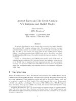
In Figure 2 we compare the “last” values of two two-year swap rates, the first paying
quarterly the three-month LIBOR rate, the second paying semiannually the six-month
LIBOR rate, from November 14th, 2005 to November 12, 2008. Again, we can notice the
change in behavior occurred in August 2007.
In Figure 3 we compare the “last” values of 3x6 EONIA forward rates and 3x6 FRA

rates, from November 14th, 2005 to November 12, 2008. Once again, these rates have been
rather aligned until August 2007, but diverged heavily thereafter.
2.1 Divergence between FRA rates and forward rates implied by
deposits
The closing values of the three-month and six-month deposits on November 12, 2008 were,
respectively, 4.286% and 4.345%. Assuming, for simplicity, 30/360 as day-count convention
(the actual one for the EUR LIBOR rate is ACT/360), the implied three-month forward
rate in three months is 4.357%, whereas the value of the corresponding FRA rate was
1.5% lower, quoted at 2.85%. Surprisingly enough, these values do not necessarily lead to
arbitrage opportunities. In fact, let us denote the FRA rate and the forward rate implied
by the two deposits with maturity T
1
and T
2
by F
X
and F
D
, respectively, and assume that
F
D
> F
X
. One may then be tempted to implement the following strategy (τ
1,2
is the year
fraction for (T
1
, T
2

]):
a) Buy (1 + τ
1,2
F
D
) bonds with maturity T
2
, paying
(1 + τ
1,2
F
D
)D(0, T
2
) = D(0, T
1
)
4
Futures rates are less straightforward to compare because of their fixed IMM maturities and their
implicit convexity correction. Their values, however, tend to be rather close to the corresp onding FRA
rates, not displaying the large discrepancies observed with other rates.
5
Figure 1: Euro 1m EONIA rates vs 1m deposit rates, from 14 Nov 2005 to 12 Nov 2008.
Source: Bloomberg.
dollars, where D(0, T) denotes the time-0 bond price for maturity T ;
b) Sell 1 bond with maturity T
1
, receiving D(0, T
1
) dollars;

c) Enter a (payer) FRA, paying out at time T
1
τ
1,2
(L(T
1
, T
2
) − F
X
)
1 + τ
1,2
L(T
1
, T
2
)
where L(T
1
, T
2
) is the LIBOR rate set at T
1
for maturity T
2
.
The value of this strategy at the current time is zero. At time T
1
, b) plus c) yield

τ
1,2
(L(T
1
, T
2
) − F
X
)
1 + τ
1,2
L(T
1
, T
2
)
− 1 = −
1 + τ
1,2
F
X
1 + τ
1,2
L(T
1
, T
2
)
,
which is negative if rates are assumed to be positive. To pay this residual debt, we sell the

1 + τ
1,2
F
D
bonds with maturity T
2
, remaining with
1 + τ
1,2
F
D
1 + τ
1,2
L(T
1
, T
2
)
−
1 + τ
1,2
F
X
1 + τ
1,2
L(T
1
, T
2
)

=
τ
1,2
(F
D
− F
X
)
1 + τ
1,2
L(T
1
, T
2
)
> 0
in cash at T
1
, which is equivalent to τ
1,2
(F
D
− F
X
) received at
2
. This is clearly an
arbitrage, since a zero investment today produces a (stochastic but) positive gain at time
T
1

or, equivalently, a deterministic positive gain at T
2
(with no intermediate net cash
6
Figure 2: Euro 2y swap rates (3m vs 6m), from 14 Nov 2005 to 12 Nov 2008. Source:
Bloomberg.
flows). However, there are two issues that, in the current market environment, can not b e
neglected any more (we assume that the FRA is default-free):
i) Possibility of default before T
2
of the counterparty we lent money to;
ii) Possibility of liquidity crunch at times 0 or T
1
.
If either events occ ur, we can end up with a loss at final time T
2
that may outvalue the
positive gain τ
1,2
(F
D
− F
X
).
5
Therefore, we can conclude that the strategy above does
not necessarily constitute an arbitrage opportunity. The forward rates F
D
and F
X

are in
fact “allowed” to diverge, and their difference can be seen as representative of the market
estimate of future credit and liquidity issues.
2.2 Explaining the diffe rence in value of similar rates
The difference in value between formerly equivalent rates can be explained by means of a
simple credit model, which is based on assuming that the generic interbank counterparty
is subject to default risk.
6
To this end, let us denote by τ
t
the default time of the generic
5
Even assuming we can sell back at T
1
the T
2
-bonds to the counterparty we initially lent money to,
default still plays against us.
6
Morini (2008) develops a similar approach with stochastic probability of default. In addition to ours,
he considers bilateral default risk. His interbank counterparty is, however, kept the same, and his definition
of FRA contract is different than that used by the market.
7
Figure 3: 3x6 EONIA forward rates vs 3x6 FRA rates, from 14 Nov 2005 to 12 Nov 2008.
Source: Bloomberg.
interbank counterparty at time t, where the subscript t indicates that the random variable
τ
t
can be different at different times. Assuming independence between default and interest
rates and denoting by R the (assumed constant) recovery rate, the value at time t of a

deposit starting at that time and with maturity T is
D(t, T ) = E

e
−

T
t
r(u) du

R+(1−R)1
{τ
t
>T }

|F
t

= RP (t, T )+(1−R)P (t, T )E

1
{τ
t
>T }
|F
t

,
where E denotes expectation under the risk-neutral measure, r the default-free instan-
taneous interest rate, P (t, T ) the price of a default-free zero coupon bond at time t for

maturity T and F
t
is the information available in the market at time t.
7
Setting
Q(t, T) := E

1
{τ
t
>T }
|F
t

,
the LIBOR rate L(T
1
, T
2
), which is the simple interest earned by the deposit D(T
1
, T
2
), is
given by
L(T
1
, T
2
) =

1
τ
1,2

1
D(T
1
, T
2
)
− 1

=
1
τ
1,2

1
P (T
1
, T
2
)
1
R + (1 − R)Q(T
1
, T
2
)
− 1


.
7
We also refer to the next section for all definitions and notations.
8
Assuming that the above FRA has no counterparty risk, its time-0 value can be written as
0 = E

e
−

T
1
0
r(u) du
τ
1,2
(L(T
1
, T
2
) − F
X
)
1 + τ
1,2
L(T
1
, T
2

)

= E

e
−

T
1
0
r(u) du

1 −
1 + τ
1,2
F
X
1 + τ
1,2
L(T
1
, T
2
)

= E

e
−


T
1
0
r(u) du

1 − (1 + τ
1,2
F
X
)P (T
1
, T
2
)(R + (1 − R)Q(T
1
, T
2
))


= P (0, T
1
) − (1 + τ
1,2
F
X
)P (0, T
2
)


R + (1 − R)E

Q(T
1
, T
2
)

which yields the value of the FRA rate F
X
:
F
X
=
1
τ
1,2

P (0, T
1
)
P (0, T
2
)
1
R + (1 − R)E

Q(T
1
, T

2
)

− 1

.
Since
0 ≤ R ≤ 1, 0 < Q(T
1
, T
2
) < 1,
then
0 < R + (1 − R)E

Q(T
1
, T
2
)

< 1
so that
F
X
>
1
τ
1,2


P (0, T
1
)
P (0, T
2
)
− 1

. (1)
Therefore, the FRA rate F
X
is larger than the forward rate implied by the default-free
bonds P (0, T
1
) and P (0, T
2
).
If the OIS (EONIA) swap curve is elected to be the risk-free curve, which is reasonable
since the credit risk in an overnight rate is deemed to be negligible even in this new market
situation, then (1) explains that the FRA rate F
X
can be (arbitrarily) higher than the
corresponding forward OIS rate if the default risk implicit in the LIBOR rate is taken into
account. Similarly, the forward rate implied by the two deposits D(0, T
1
) and D(0, T
2
), i.e.
F
D

=
1
τ
1,2

D(0, T
1
)
D(0, T
2
)
− 1

=
1
τ
1,2

R + (1 − R)Q(0, T
1
)
R + (1 − R)Q(0, T
2
)
P (0, T
1
)
P (0, T
2
)

− 1

will be larger than the FRA rate F
X
if
R + (1 − R)Q(0, T
1
)
R + (1 − R)Q(0, T
2
)
>
1
R + (1 − R)E

Q(T
1
, T
2
)

.
This happens, for instance, when R < 1 and the market expectation for the future credit
premium from T
1
to T
2
(inversely proportional to Q(T
1
, T

2
)) is low compared to the value
implied by the spot quantities Q(0, T
1
) and Q(0, T
2
).
8
8
Even though the quantities Q(T
1
, T
2
) and Q(0, T
i
), i = 1, 2, refer to different default times τ
0
and
τ
T
1
, they can not be regarded as completely unrelated to each other, since they both depend on the credit
worthiness of the generic interbank counterparty from T
1
to T
2
.
9
Further degrees of freedom to be calibrated to market quotes can be added by also
modeling liquidity risk.

9
A thorough and sensible treatment of liquidity effects, is however
beyond the scope of this work.
2.3 Using multiple curves
The analysis just performed is meant to provide a simple theoretical justification for the
current divergence of market rates that refer to the same time interval. Such rates, in fact,
become compatible with each other as soon as credit and liquidity risks are taken into
account. However, instead of explicitly modeling credit and liquidity effects, practitioners
seem to deal with the above discrepancies by segmenting market rates, labeling them
differently according to their application period. This results in the construction of different
zero-coupon curves, one for each possible rate length considered. One of this curves, or any
version obtained by mixing “inhomogeneous rates”, is then elected to act as the discount
curve.
As far as derivatives pricing is concerned, however, it is still not clear how to account for
these new market features and practice. Whe n pricing interest rate derivatives with a given
model, the usual first step is the model calibration to the term structure of market rates.
This task, before August 2007, was straightforward to accomplish thanks to the existence
of a unique, well defined yield curve. When dealing with multiple curves, however, not
only the calibration to market rates but also the modeling of their evolution becomes a
non-trivial task. To this end, one may identify two possible solutions:
i) Modeling default-free rates in conjunction with default times τ
t
and/or liquidity
effects.
ii) Modeling the j oint, but distinct, evolution of rates that applies to the same interval.
The former choice is consistent with the above procedure to justify the simultaneous
existence of formerly equivalent rates. Howeve r, devising a sensible model for the evolution
of default times may not be so obvious. Notice, in fact, that the standard theories on credit
risk do not immediately apply here, since the default time does not refer to a single credit
entity, but it is representative of a generic sector, the interbank one. The random variable

τ
t
, therefore, does not change over time because the credit worthiness of the reference entity
evolves stochastically, but because the counterparty is generic and a new default time τ
t
is
generated at each time t to assess the credit premium in the LIBOR rate at that time.
In this article, we prefer to follow the latter approach and apply a logic similar to that
used in the yield curves construction. In fact, given that practitioners build different curves
for different tenors, it is quite reasonable to introduce an interest rate model where such
curves are modeled jointly but distinctly. To this end, we will model forward rates with a
given tenor in conjunction with those implied by the discount curve. This will be achieved
in the spirit of Kijima et al (2008).
The forward (or ”growth”) curve associated to a given rate tenor can be constructed
with standard bootstrapping techniques. The main difference with the methodology fol-
9
Liquidity effects are modeled, among others, by Cetin et al. (2006) and Acerbi and Scandolo (2007).
10
lowed in the pre-credit-crunch situation is that now only the market quotes corresponding
to the given tenor are employed in the stripping procedure. For instance, the three-month
curve can be constructed by bootstrapping zero-coupon rates from the market quotes of
the three-month deposit, the futures (or 3m FRAs) for the main maturities and the liquid
swaps (vs 3m).
The discount curve, instead, can be selected in several different ways, depending on the
contract to price. For instance, in absence of c ounterparty risk or in case of collateralized
derivatives, it can be deemed to be the classic risk-neutral curve, whose best proxy is the
OIS swap curve, obtained by suitably interpolating and extrapolating OIS swap quotes.
10
For a contract signed with a generic interbank counterparty without collateral, the discount
curve should reflect the f act that future cash flows are at risk and, as such, must be

discounted at LIBOR, which is the rate reflecting the credit risk of the interbank sector.
In such a case, therefore, the discount curve may be bootstrapped (and extrapolated) from
the quoted deposit rates. In general, the discount curve can be selected as the yield curve
associated the counterparty in question.
11
In the following, we will assume that future cash flows are all discounted with the same
discount curve. The extension to a more general case involves a heavier notation and here
neglected for simplicity.
3 Basic definitions and notation
Let us assume that, in a single currency economy, we have selected N different interest-rate
lengths δ
1
, . . . , δ
N
and constructed the corresponding yield curves. The curve associated
to length δ
i
will be shortly referred to as curve i.
12
We denote by P
i
(t, T) the associated
discount factor (equivalently, zero-coup on bond price) at time t for maturity T. We also
assume we are given a curve D for discounting future cash flows. We denote by P
D
(t, T)
the curve-D discount factor at time t for maturity T .
We will consider the time structures {T
i
0

, T
i
1
, . . .}, where the superscript i denotes the
curve it belongs to, and {T
S
0
, T
S
1
, . . .}, which includes the payment times of a swap’s fixed
leg.
Forward rates can be defined for each given curve. Precisely, for each curve x ∈
{1, 2, . . . , N, D}, the (simply-compounded) forward rate prevailing at time t and applied
to the future time interval [T, S] is defined by
F
x
(t; T, S) :=
1
τ
x
(T, S)

P
x
(t, T)
P
x
(t, S)
− 1


, (2)
10
Notice that OIS rates carry the credit risk of an ove rnight rate, which may be regarded as negligible
in most situations.
11
A detailed description of a possible methodology for constructing forward and discount curves is
outlined in Ametrano and Bianchetti (2008). In general, bootstrapping multiple curves, for the same
currency, involves plenty of technicalities and subjective choices.
12
In the next section, we will hint at a possible bootstrap methodology.
11
where τ
x
(T, S) is the year fraction for the interval [T, S] under the convention of curve x.
13
Given the times t ≤ T
i
k−1
< T
i
k
and the curve x ∈ {1, . . . , N, D}, we will make use of
the following short-hand notation:
F
x
k
(t) := F
x
(t; T

i
k−1
, T
i
k
) =
1
τ
x
k

P
x
(t, T
i
k−1
)
P
x
(t, T
i
k
)
− 1

(3)
where τ
x
k
is the year fraction for the interval [T

i
k−1
, T
i
k
] for curve x, namely τ
x
k
:= τ
x
(T
i
k−1
, T
i
k
).
As in Kijima et al (2008), the pricing measures we will consider are those asso ciated to
the discount curve D. To denote these measures we will adopt the notation Q
z
x
, where the
subscript x (mainly D) identifies the underlying yield curve, and the superscript z defines
the measure in question. More precisely, we denote by:
• Q
T
D
the T -forward measure, whose numeraire is the zero-coupon bond P
D
(·, T).

• Q
T
D
the spot LIBOR measure associated to times T = {T
i
0
, . . . , T
i
M
} , whose numeraire
is the discretely-rebalanced bank account B
T
D
:
B
T
D
(t) =
P
D
(t, T
i
m
)

m
j=0
P
D
(T

i
j−1
, T
i
j
)
, T
i
m−1
< t ≤ T
i
m
, m = 1, . . . , M.
• Q
c,d
D
the forward swap measure defined by the time structure {T
S
c
, T
S
c+1
, . . . , T
S
d
},
whose numeraire is the annuity
C
c,d
D

(t) =
d

j=c+1
τ
S
j
P
D
(t, T
S
j
),
where τ
S
j
:= τ
D
(T
S
j−1
, T
S
j
).
The expectation under the generic measure Q
z
x
will be denoted by E
z

x
, where again the in-
dices x and z identify, respectively, the underlying yield curve and the measure in question.
The information available in the market at each time t will be described by the filtration
F
t
.
4 The valuation of interest rate swaps
In this section, we show how to value linear interest rate derivatives under our assumption
of distinct forward and discount curves. To this end, let us consider a set of times T
i
a
, . . . , T
i
b
compatible with c urve i,
14
and an interest rate swap where the floating leg pays at e ach
13
In practice, for curves i = 1, . . . , N , we will consider only intervals where S = T +δ
i
, whereas for curve
D the interval [S, T ] may be totally arbitrary.
14
For instance, if i denotes the three-month curve, then the times T
i
k
must be three-month spaced.
12
time T

i
k
the LIBOR rate of curve i set at the previous time T
i
k−1
, k = a + 1, . . . , b. In
formulas, the time-T
i
k
payoff of the floating leg is
FL(T
i
k
; T
i
k−1
, T
i
k
) = τ
i
k
F
i
k
(T
i
k−1
) =
1

P
i
(T
i
k−1
, T
i
k
)
− 1. (4)
The time-t value, FL(t; T
i
k−1
, T
i
k
), of such a payoff can be obtained by taking the discounted
expectation under the forward measure Q
T
i
k
D
:
15
FL(t; T
i
k−1
, T
i
k

) = τ
i
k
P
D
(t, T
i
k
)E
T
i
k
D

F
i
k
(T
i
k−1
)|F
t

.
Defining the time-t FRA rate as the fixed rate to be exchanged at time T
i
k
for the floating
payment (4) so that the swap has zero value at time t,
16

i.e
L
i
k
(t) := FRA(t; T
i
k−1
, T
i
k
) = E
T
i
k
D

F
i
k
(T
i
k−1
)|F
t

,
we can write
FL(t; T
i
k−1

, T
i
k
) = τ
i
k
P
D
(t, T
i
k
)L
i
k
(t). (5)
In the classic single curve valuation (i ≡ D), the forward rate F
i
k
is a martingale under
the associated T
i
k
-forward measure (coinciding with Q
T
i
k
D
), so that the expected value L
i
k

(t)
coincides with the current forward rate:
L
i
k
(t) = F
i
k
(t).
Accordingly, as is well known, the present value of each payment in the swap’s floating leg
can be simplified as follows:
FL(t; T
i
k−1
, T
i
k
) = τ
i
k
P
D
(t, T
i
k
)L
i
k
(t) = τ
i

k
P
i
(t, T
i
k
)F
i
k
(t) = P
i
(t, T
i
k−1
) − P
i
(t, T
i
k
),
which leads to the classic result that the LIBOR rate set at time T
i
k−1
and paid at time
T
i
k
can be replicated by a long position in a zero-coupon bond expiring at time T
i
k−1

and a
short position in another bond with maturity T
i
k
.
In the situation we are dealing with, however, curves i and D are different, in general.
The forward rate F
i
k
is not a martingale under the forward measure Q
T
i
k
D
, and the FRA
rate L
i
k
(t) is different from F
i
k
(t). Therefore, the present value of a future LIBOR rate is
no longer obtained by discounting the corresponding forward rate, but by discounting the
corresponding FRA rate.
15
For most swaps, thanks to the presence of collaterals or netting clauses, curve D can be assumed to
be the risk-free one (as obtained from OIS swap rates).
16
This FRA rate is slightly different than that defined by the marke t, see Section 2.2. This slight abuse
of terminology is justified by the definition that applies when payments occur at the end of the application

period (like in this case).
13
The net present value of the swap’s floating le g is simply given by summing the values
(5) of single payments:
FL(t; T
i
a
, . . . , T
i
b
) =
b

k=a+1
FL(t; T
i
k−1
, T
i
k
) =
b

k=a+1
τ
i
k
P
D
(t, T

i
k
)L
i
k
(t), (6)
which, for the reasons just explained, will be different in general than P
D
(t, T
i
a
) − P
D
(t, T
i
b
)
or P
i
(t, T
i
a
) − P
i
(t, T
i
b
).
Let us then consider the swap’s fixed leg and denote by K the fixed rate paid on the
fixed leg’s dates T

S
c
, . . . , T
S
d
. The present value of these payments is immediately obtained
by discounting them with the discount curve D:
d

j=c+1
τ
S
j
KP
D
(t, T
S
j
) = K
d

j=c+1
τ
S
j
P
D
(t, T
S
j

),
where we remember that τ
S
j
= τ
D
(T
S
j−1
, T
S
j
).
Therefore, the interest rate swap value, to the fixed-rate payer, is given by
IRS(t, K; T
i
a
, . . . , T
i
b
, T
S
c
, . . . , T
S
c
) =
b

k=a+1

τ
i
k
P
D
(t, T
i
k
)L
i
k
(t) − K
d

j=c+1
τ
S
j
P
D
(t, T
S
j
).
We can then calculate the corresponding forward swap rate as the fixed rate K that makes
the IRS value equal to zero at time t. We get:
S
i
a,b,c,d
(t) =


b
k=a+1
τ
i
k
P
D
(t, T
i
k
)L
i
k
(t)

d
j=c+1
τ
S
j
P
D
(t, T
S
j
)
. (7)
This is the forward swap rate of an interest rate swap where cash flows are generated
through curve i and discounted with curve D.

In the particular case of a spot-starting swap, with payment times for the floating and
fixed legs given, respectively, by T
i
1
, . . . , T
i
b
and T
S
1
, . . . , T
S
d
, with T
i
b
= T
S
d
, the swap rate
becomes:
S
i
0,b,0,d
(0) =

b
k=1
τ
i

k
P
D
(0, T
i
k
)L
i
k
(0)

d
j=1
τ
S
j
P
D
(0, T
S
j
)
, (8)
where L
1
(0) is the constant first floating payment (known at time 0). As already noticed
by Kijima et at. (2008), neither leg of a spot-starting swap needs be worth par (when a
fictitious exchange of notionals is introduced at maturity). However, this is not a problem,
since the only requirement for quoted spot-starting swaps is that their net present value
must be equal to zero.

Remark 1 As traditionally done in any bootstrapping algorithm, equation (8) can be used
to infer the expected rates L
i
k
implied by the market quotes of spot-starting swaps, which by
14
definition have zero value. The bootstrapped L
i
k
can then be used, in conjunction with any
interpolation tool, to price other swaps based on curve i. As already noticed by Boenkost
and Schmidt (2005) and by Kijima et al. (2008), these other swaps will have different
values, in general, than those obtained through classic bootstrapping methods applied to
swap rates
S
0,d
(0) =
1 − P
D
(0, T
S
d
)

d
j=1
τ
S
j
P

D
(0, T
S
j
)
.
However, this is perfectly reasonable since we are here using an alternative, and more
general, approach.
5 The pricing of caplets and swaptions
Similarly to what we just did for interest rate swaps, the purpose of this section is to derive
pricing formulas for options on the main interest rates, which will result in modifications
of the corresponding Black-like formulas governed by our double-curve paradigm.
As is well known, the formal justifications for the use of Black-like formulas for caps
and swaptions come, respectively, from the lognormal LMM of Brace et al. (1997) and
Miltersen et al. (1997) and the lognormal swap model of Jamshidian (1997).
17
To be able
to adapt such formulas to our double-curve case, we will have to reformulate accordingly
the corresponding market models.
Again, the choice of the discount curve D depends on the credit worthiness of the
counterparty and on the possible presence of a collateral mitigating the credit risk exposure.
5.1 Market formula for caplets
We first consider the case of a caplet paying out at time T
i
k
τ
i
k
[F
i

k
(T
i
k−1
) − K]
+
. (9)
To price such payoff in the basic single-curve case, one notices that the forward rate F
i
k
is
a martingale under the T
i
k
-forward measure Q
T
i
k
i
for curve i, and then calculates the time-t
caplet price
Cplt(t, K; T
i
k−1
, T
i
k
) = τ
i
k

P
i
(t, T
i
k
)E
T
i
k
i

[F
i
k
(T
i
k−1
) − K]
+
|F
t

according to the chosen dynamics. For instance, the classic choice of a driftless geometric
Brownian motion
18
dF
i
k
(t) = σ
k

F
i
k
(t) dZ
k
(t), t ≤ T
i
k−1
,
17
It is worth mentioning that the first proof that Black-like formulas for caps and swaptions are arbitrage
free is due to Jamshidian (1996).
18
We will use the symbol “d” to denote differentials as opposed to d, which instead denotes the index
of the final date in the swap’s fixed leg.
15
where σ
k
is a constant and Z
k
is a Q
T
i
k
i
-Brownian motion, leads to Black’s pricing formula:
Cplt(t, K; T
i
k−1
, T

i
k
) = τ
i
k
P
i
(t, T
i
k
) Bl

K, F
i
k
(t), σ
k

T
i
k−1
− t

(10)
where
Bl(K, F, v) = F Φ

ln(F/K) + v
2
/2

v

− KΦ

ln(F/K) − v
2
/2
v

,
and Φ denotes the standard normal distribution function.
In our double-curve setting, the caplet valuation requires more attention. In fact, since
the pricing measure is now the forward measure Q
T
i
k
D
for curve D, the caplet price at time
t becomes
Cplt(t, K; T
i
k−1
, T
i
k
) = τ
i
k
P
D

(t, T
i
k
)E
T
i
k
D

[F
i
k
(T
i
k−1
) − K]
+
|F
t

.
As already explained in the IRS case, the problem with this new expectation is that the
forward rate F
i
k
is not, in general, a martingale under Q
T
i
k
D

. A possible way to value it is
to model the dynamics of F
i
k
under its own measure Q
T
i
k
i
and then to model the Radon-
Nikodym derivative dQ
T
i
k
i
/dQ
T
i
k
D
that defines the measure change from Q
T
i
k
i
to Q
T
i
k
D

. This
is the approach proposed by Bianchetti (2008), who uses a foreign-currency analogy and
derives a quanto-like correction for the drift of F
i
k
. Here, instead, we take a different route.
Our idea is to follow a conceptually similar approach as in the classic LMM. There, the
trick was to replace the LIBOR rate entering the caplet payoff with the equivalent forward
rate, since the latter has “better” dynamics (a martingale) under the reference pricing
measure. Here, we make a step forward, and replace the forward rate with its conditional
expected value (the FRA rate). The purpose is the same as before, namely to introduce
an underlying asset whose dynamics is easier to model.
Since
L
i
k
(t) = E
T
i
k
D

F
i
k
(T
i
k−1
)|F
t


,
at the reset time T
i
k−1
the two rates F
i
k
and L
i
k
coincides:
L
i
k
(T
i
k−1
) = F
i
k
(T
i
k−1
).
We can, therefore, replace the payoff (9) with
τ
i
k
[L

i
k
(T
i
k−1
) − K]
+
(11)
and view the caplet as a call option no more on F
i
k
(T
i
k−1
) but on L
i
k
(T
i
k−1
). This leads to:
Cplt(t, K; T
i
k−1
, T
i
k
) = τ
i
k

P
D
(t, T
i
k
)E
T
i
k
D

[L
i
k
(T
i
k−1
) − K]
+
|F
t

. (12)
The FRA rate L
i
k
(t) is, by definition, a martingale under the measure Q
T
i
k

D
. If we smartly
choose the dynamics of such a rate, we can value the last expectation analytically and
16
obtain a closed-form formula for the caplet price. For instance, the obvious choice of a
driftless geometric Brownian motion
dL
i
k
(t) = v
k
L
i
k
(t) dZ
k
(t), t ≤ T
i
k−1
where v
k
is a constant and Z
k
is now a Q
T
i
k
D
-Brownian motion, leads to the following pricing
formula:

Cplt(t, K; T
i
k−1
, T
i
k
) = τ
i
k
P
D
(t, T
i
k
) Bl

K, L
i
k
(t), v
k

T
i
k−1
− t

.
Therefore, under lognormal dynamics for the rate L
i

k
, the caplet price is again given by
Black’s formula with an implied volatility v
k
. The differences with respect to the classic
formula (10) are give n by the underlying rate, which here is the FRA rate L
i
k
, and by the
discount factor, which here belongs to curve D.
5.2 Market formula for swaptions
The other plain-vanilla option in the interest rate market is the European swaption. A
payer swaption gives the right to enter at time T
i
a
= T
S
c
an IRS with payment times for the
floating and fixed legs given, respectively, by T
i
a+1
, . . . , T
i
b
and T
S
c+1
, . . . , T
S

d
, with T
i
b
= T
S
d
and where the fixed rate is K. Its payoff at time T
i
a
= T
S
c
is therefore

S
i
a,b,c,d
(T
i
a
) − K

+
d

j=c+1
τ
S
j

P
D
(T
S
c
, T
S
j
), (13)
where, see (7),
S
i
a,b,c,d
(t) =

b
k=a+1
τ
i
k
P
D
(t, T
i
k
)L
i
k
(t)


d
j=c+1
τ
S
j
P
D
(t, T
S
j
)
.
Setting
C
c,d
D
(t) =
d

j=c+1
τ
S
j
P
D
(t, T
S
j
)
the payoff (13) is conveniently priced under the swap measure Q

c,d
D
, whose associated
numeraire is the annuity C
c,d
D
(t). In fact, we get:
PS(t, K; T
i
a+1
, . . . , T
i
b
, T
S
c+1
, . . . , T
S
d
)
=
d

j=c+1
τ
S
j
P
D
(t, T

S
j
) E
Q
c,d
D


S
i
a,b,c,d
(T
i
a
) − K

+

d
j=c+1
τ
S
j
P
D
(T
S
c
, T
S

j
)
C
c,d
D
(T
S
c
)
|F
t

=
d

j=c+1
τ
S
j
P
D
(t, T
S
j
) E
Q
c,d
D

S

i
a,b,c,d
(T
i
a
) − K

+
|F
t

(14)
so that, also in our multi-curve paradigm, pricing a swaption is equivalent to pricing an
option on the underlying swap rate.
17
As in the single-curve case, the forward swap rate S
i
a,b,c,d
(t) is a martingale under the
swap measure Q
c,d
D
. In fact, by (6), S
i
a,b,c,d
(t) is equal to a tradable asset (the floating leg
of the swap) divided by the numeraire C
c,d
D
(t):

S
i
a,b,c,d
(t) =

b
k=a+1
τ
i
k
P
D
(t, T
i
k
)L
i
k
(t)

d
j=c+1
τ
S
j
P
D
(t, T
S
j

)
=
FL(t; T
i
a
, . . . , T
i
b
)
C
c,d
D
(t)
. (15)
Assuming that the swap rate S
i
a,b,c,d
evolves, under Q
c,d
D
, according to a driftless geometric
Brownian motion:
dS
i
a,b,c,d
(t) = ν
a,b,c,d
S
i
a,b,c,d

(t) dZ
a,b,c,d
(t), t ≤ T
i
a
where ν
a,b,c,d
is a constant and Z
a,b,c,d
is a Q
c,d
D
-Brownian motion, the expectation in (14)
can be explicitly calculated as in the caplet case, leading to the generalized Black formula:
PS(t, K; T
i
a+1
, . . . , T
i
b
, T
S
c+1
, . . . , T
S
d
) =
d

j=c+1

τ
S
j
P
D
(t, T
S
j
) Bl

K, S
i
a,b,c,d
(t), ν
a,b,c,d

T
i
a
− t

.
Therefore, the double-curve swaption price is still given by a Black-like formula, with the
only differences with respect to the basic case that discounting is done through curve D
and that the swap rate S
i
a,b,c,d
(t) has a more general definition.
After having derived market formulas for caps and swaptions under distinct discount
and forward curve s, we are now ready to extend the basic LMMs. We start by considering

the fundamental case of lognormal dynamics, and then introduce stochastic volatility in a
rather general fashion.
6 The double-curve lognormal LMM
In the classic (single-curve) LMM, one models the joint evolution of a set of consecutive
forward LIBOR rates under a common pricing measure, typically some “terminal” forward
measure or the spot LIBOR measure corresponding to the set of times defining the family
of forward rates. Denoting by T = {T
i
0
, . . . , T
i
M
} the times in question, one then jointly
models rates F
i
k
, k = 1, . . . , M, under the forward measure Q
T
i
M
i
or under the spot LIBOR
measure Q
T
i
. Using measure change techniques, one finally derives pricing formulas for
the main calibration instruments (caps and swaptions) either in closed form or through
efficient approximations.
To extend the LMM to the multi-curve case, we first need to identify the rates we need
to model. The previous section suggests that the FRA rates L

i
k
are convenient rates to
model as soon as we have to price a payoff, like that of a caplet, which depends on LIBOR
18
rates belonging to the same curve i. Moreover, in case of a swap-rate dependent payoff,
we notice we can write
S
i
a,b,c,d
(t) =

b
k=a+1
τ
i
k
P
D
(t, T
i
k
)L
i
k
(t)

d
j=c+1
τ

S
j
P
D
(t, T
S
j
)
=
b

k=a+1
ω
k
(t)L
i
k
(t), (16)
where the weights ω
k
are defined by
ω
k
(t) :=
τ
i
k
P
D
(t, T

i
k
)

d
j=c+1
τ
S
j
P
D
(t, T
S
j
)
. (17)
Characterizing the forward swap rate S
i
a,b,c,d
(t) as a linear combination of FRA rates L
i
k
(t)
gives another argument supporting the modeling of FRA rates as fundamental bricks to
generate sensible future payoffs in the pricing of interest rate derivatives. Notice, also the
consistency with the standard single-curve case, where the forward LIBOR rates F
i
k
(t) and
the FRA rates L

i
k
(t) coincide by definition.
However, there is a major difference with respect to the single-curve case, namely that
forward rates belonging to the discount curve need to be modeled too. In fact, as is evident
from equation (16), future swap rates also depend on future discount factors which, unless
we unrealistically assume a deterministic discount curve, will evolve stochastically over
time. Moreover, we will show below that the dynamics of FRA rates under typical pricing
measures depend on forward rates of curve D, so that also path-dependent payoffs on
LIBOR rates will depend on the dynamics of the discount curve.
6.1 The model dynamics
The LMM was introduced in the financial literature by Brace et al. (1997) and Miltersen
et al. (1997) by assuming that forward LIBOR rates have a lognormal-type diffusion coef-
ficient.
19
Here, we extend their approach to the case where the curve used for discounting
is different than that used to generate the relevant future rates. For simplicity, we stick to
the case where these rates belong to the same curve i.
Let us consider a set of times T = {0 < T
i
0
, . . . , T
i
M
}, which we assume to be compatible
with curve i. We assume that each rate L
i
k
(t) evolves, under its canonical forward measure
Q

T
i
k
D
, as a driftless geometric Brownian motion:
dL
i
k
(t) = σ
k
(t)L
i
k
(t) dZ
k
(t), t ≤ T
i
k−1
(18)
where the instantaneous volatility σ
k
(t) is deterministic and Z
k
is the k-th component of an
M-dimensional Q
T
i
k
D
-Brownian motion Z with instantaneous correlation matrix (ρ

k,j
)
k,j=1, ,M
,
namely dZ
k
(t) dZ
j
(t) = ρ
k,j
dt.
19
This implies that each forward LIBOR rate evolves according to a geometric Brownian motion under
its associated forward measure.
19
In a double-curve setting, we also need to model the evolution of rates
F
D
k
(t) = F
D
(t; T
i
k−1
, T
i
k
) =
1
τ

D
k

P
D
(t, T
i
k−1
)
P
D
(t, T
i
k
)
− 1

τ
D
k
= τ
D
(T
i
k−1
, T
i
k
)
To this end, we assume that the dynamics of each rate F

D
h
under the associated forward
measure Q
T
i
h
D
is given by:
dF
D
h
(t) = σ
D
h
(t)F
D
h
(t) dZ
D
h
(t), t ≤ T
i
h−1
(19)
where the instantaneous volatility σ
D
h
(t) is deterministic and Z
D

h
is the h-th component of
an M-dimensional Q
T
i
h
D
-Brownian motion Z
D
whose correlations are
dZ
D
k
(t) dZ
D
h
(t) = ρ
D,D
k,h
dt
dZ
k
(t) dZ
D
h
(t) = ρ
i,D
k,h
dt
Clearly, correlations ρ = (ρ

k,j
)
k,j=1, ,M
, ρ
D,D
= (ρ
D,D
k,h
)
k,h=1, ,M
and ρ
i,D
= (ρ
i,D
k,h
)
k,h=1, ,M
must be chosen so as to ensure that the global matrix
R :=

ρ ρ
i,D

ρ
i,D


ρ
D,D


is positive (semi)definite.
Remark 2 In some situations, it may be more realistic to resort to an alternative approach
and model either curve i or D jointly with the spread between them, see e.g. Kijima (2008)
or Sch¨onbucher (2000). This happens, for instance, when one curve is above the other and
there are sound financial reasons why the spread should be preserved positive in the future.
In such a case, one can assume that each spread X
k
(t) := |L
i
k
(t) − F
D
k
(t)| evolves under
the corresponding forward measure Q
T
i
k
D
, according to some
dX
k
(t) = σ
X
k
(t, X
k
(t)) dZ
X
k

(t),
whose solution is positively distributed. Sticking to (18), the dynamics (19) of forward rates
F
D
k
must then be replaced with
dF
D
k
(t) = dL
i
k
(t) ± dX
k
(t),
where the sign ± depends on the relative position of curves i and D. The analysis that
follows can be equivalently applied to the new dynamics of rates F
D
k
.
20
20
The calculations are essentially the same. Their length depends on the chosen volatility function σ
X
k
.
20
6.2 Dynamics under a general forward measure
To derive the dynamics of the FRA rate L
i

k
(t) under the forward measure Q
T
i
j
D
we start
from (18) and perform a change of measure from Q
T
i
k
D
to Q
T
i
j
D
, whose associated numeraires
are the curve-D zero-coupon bonds with maturities T
i
k
and T
i
j
, respectively. To this end,
we apply the change-of-numeraire formula relating the drifts of a given process under two
measures with known numeraires, see for instance Brigo and Mercurio (2006). The drift of
L
i
k

(t) under Q
T
i
j
D
is then equal to
Drift(L
i
k
; Q
T
i
j
D
) = −
dL
i
k
, ln(P
D
(·, T
i
k
)/P
D
(·, T
i
j
))
t

dt
,
where X, Y 
t
denotes the instantaneous covariation between processes X and Y at time
t.
Let us first consider the case j < k. The log of the ratio of the two numeraires can be
written as
ln(P
D
(t, T
i
k
)/P
D
(t, T
i
j
)) = ln

1/

k

h=j+1
(1 + τ
D
h
F
D

h
(t))

= −
k

h=j+1
ln

1 + τ
D
h
F
D
h
(t)

from which we get:
Drift(L
i
k
; Q
T
i
j
D
) = −
dL
i
k

, ln(P
D
(·, T
i
k
)/P
D
(·, T
i
j
))
t
dt
=
k

h=j+1
dL
i
k
, ln

1 + τ
D
h
F
D
h



t
dt
=
k

h=j+1
τ
D
h
1 + τ
D
h
F
D
h
(t)
dL
i
k
, F
D
h

t
dt
.
In the standard LMM, the drift term of L
i
k
under Q

T
i
j
D
depends on the instantaneous
covariations between forward rates F
i
k
and F
i
h
, h = j + 1, . . . , k. The initial assumptions
on the joint dynamics of forward rates are therefore sufficient to determine such a drift
term. Here, however, the situation is different since rates L
i
k
and F
D
h
belong, in general, to
different curves, and to calculate the instantaneous covariations in the drift term, we also
need the dynamics of rates F
D
h
.
Under (19), we thus obtain
Drift(L
i
k
; Q

T
i
j
D
) = σ
k
(t)L
i
k
(t)
k

h=j+1
ρ
i,D
k,h
τ
D
h
σ
D
h
(t)F
D
h
(t)
1 + τ
D
h
F

D
h
(t)
.
The derivation of the drift rate in the case j > k is perfectly analogous.
21
As to forward rates F
D
k
, their Q
T
i
j
D
-dynamics are equivalent to those we obtain in the
classic single-curve case, see Brigo and Mercurio (2006), since these probability measures
and rates are associated to the same curve D.
The joint evolution of all FRA rates L
i
1
, . . . , L
i
M
and forward rates F
D
1
, . . . , F
D
M
under

a common forward measure is then summarized in the following.
Proposition 3 The dynamics of L
i
k
and F
D
k
under the forward measure Q
T
i
j
D
in the three
cases j < k, j = k and j > k are, respectively,
j < k, t ≤ T
i
j
:














dL
i
k
(t) = σ
k
(t)L
i
k
(t)

k

h=j+1
ρ
i,D
k,h
τ
D
h
σ
D
h
(t)F
D
h
(t)
1 + τ
D
h

F
D
h
(t)
dt + dZ
j
k
(t)

dF
D
k
(t) = σ
D
k
(t)F
D
k
(t)

k

h=j+1
ρ
D,D
k,h
τ
D
h
σ

D
h
(t)F
D
h
(t)
1 + τ
D
h
F
D
h
(t)
dt + dZ
j,D
k
(t)

j = k, t ≤ T
i
k−1
:

dL
i
k
(t) = σ
k
(t)L
i

k
(t) dZ
j
k
(t)
dF
D
k
(t) = σ
D
k
(t)F
D
k
(t) dZ
j,D
k
(t)
j > k, t ≤ T
i
k−1
:












dL
i
k
(t) = σ
k
(t)L
i
k
(t)

−
j

h=k+1
ρ
i,D
k,h
τ
D
h
σ
D
h
(t)F
D
h
(t)

1 + τ
D
h
F
D
h
(t)
dt + dZ
j
k
(t)

dF
D
k
(t) = σ
D
k
(t)F
D
k
(t)

−
j

h=k+1
ρ
D,D
k,h

τ
D
h
σ
D
h
(t)F
D
h
(t)
1 + τ
D
h
F
D
h
(t)
dt + dZ
j,D
k
(t)

(20)
where Z
j
k
and Z
j,D
k
are the k-th components of M-dimensional Q

T
i
j
D
-Brownian motions Z
j
and Z
j,D
with correlation matrix R.
Remark 4 Following the same arguments used in the standard single-curve case, we can
easily prove that the SDEs (20) for the FRA rates all admit a unique strong solution if the
coefficients σ
D
h
are bounded.
When curves i and D coincide, we have already noticed that the FRA rates L
i
k
coincide
with the corresponding F
i
k
. As a further sanity check, we can also see that the FRA rate
dynamics reduce to those of the corresponding forward rates since
i ≡ D ⇒










ρ
i,D
k,h
→ ρ
k,h
τ
D
h
→ τ
i
h
σ
D
h
(t) → σ
h
(t)
F
D
h
(t) → F
i
h
(t)
for each h, k.
The extended dynamics (20) may raise some concern on numerical issues. In fact,

having doubled the number of rates to simulate, the computational burden of the lognormal
22
LMM (20) is doubled with respect to that of the single-curve case, since the SDEs for the
homologues L
i
k
and F
D
k
share the same structure. However, some smart selection of the
correlations between rates can reduce the simulation time. For instance, assuming that
ρ
i,D
k,h
= ρ
D,D
k,h
for each h, k, leads to the same drift rates for L
i
k
and the corresponding F
D
k
,
thus halvening the number of drifts to be calculated at each simulation time. This gives a
valuable advantage since it is well known that the drift calculations in a LMM are extremely
time consuming.
6.3 Dynamics under the spot LIBOR measure
Another measure commonly used for modeling the joint evolution of the given rates and
for pricing related derivatives is the spot LIBOR measure Q

T
D
associated to times T =
{T
i
0
, . . . , T
i
M
} , whose numeraire is the discretely-rebalanced bank account B
T
D
B
T
D
(t) =
P
D
(t, T
i
β(t)−1
)

β(t)−1
j=0
P
D
(T
i
j−1

, T
i
j
)
,
where β(t) = m if T
i
m−2
< t ≤ T
i
m−1
, m ≥ 1, so that t ∈ (T
i
β(t)−2
, T
i
β(t)−1
].
Application of the change-of numeraire technique, immediately leads to the following.
Proposition 5 The dynamics of FRA and forward rates under the spot LIBOR measure
Q
T
D
are given by:
dL
i
k
(t) = σ
k
(t)L

i
k
(t)
k

h=β(t)
ρ
i,D
k,h
τ
D
h
σ
D
h
(t)F
D
h
(t)
1 + τ
D
h
F
D
h
(t)
dt + σ
k
(t)L
i

k
(t) dZ
d
k
(t)
dF
D
k
(t) = σ
D
k
(t)F
D
k
(t)
k

h=β(t)
ρ
D,D
k,h
τ
D
h
σ
D
h
(t)F
D
h

(t)
1 + τ
D
h
F
D
h
(t)
dt + σ
D
k
(t)F
D
k
(t) dZ
d,D
k
(t)
(21)
where Z
d
= {Z
d
1
, . . . , Z
d
M
} and Z
d,D
= {Z

d,D
1
, . . . , Z
d,D
M
} are M-dimensional Q
T
D
-Brownian
motions with correlation matrix R.
6.4 Pricing caplets in the lognormal LMM
The pricing of caplets in the LMM is straightforward and follows from the same arguments
of Section 5. We get:
Cplt(t, K; T
i
k−1
, T
i
k
) = τ
i
k
P
D
(t, T
i
k
) Bl(K, L
i
k

(t), v
k
(t))
where
v
k
(t) :=


T
i
k−1
t
σ
k
(u)
2
du
As expected, thanks to the lognormality assumption, this formula for caplets (and hence
caps) is analogous to that obtained in the basic lognormal LMM. We just have to replace
forward rates with FRA rates and use the discount factors coming from curve D.
23
6.5 Pricing swaptions in the lognormal LMM
An analytical approximation for the implied volatility of swaptions can be derived also in
our multi-curve setting. To this end, remember (16) and (17):
S
i
a,b,c,d
(t) =
b


k=a+1
ω
k
(t)L
i
k
(t),
ω
k
(t) =
τ
i
k
P
D
(t, T
i
k
)

d
j=c+1
τ
S
j
P
D
(t, T
S

j
)
.
The forward swap rate S
i
a,b,c,d
(t) can be written as a linear combination of FRA rates L
i
k
(t).
Contrary to the single curve case, the weights are not a function of the FRA rates only,
since they also depend on discount factors calculated on curve D. Therefore we can not
write that, under the swap measure Q
c,d
D
, the swap rate S
i
a,b,c,d
(t) satisfies the S.D.E.
dS
i
a,b,c,d
(t) =
b

k=a+1
∂S
i
a,b,c,d
(t)

∂L
i
k
(t)
σ
k
(t)L
i
k
(t) dZ
c,d
k
(t).
However, we can resort to a standard approximation technique and freeze the weights ω
k
at their time-zero value. This leads to the approximation
S
i
a,b,c,d
(t) ≈
b

k=a+1
ω
k
(0)L
i
k
(t),
which enables us to write

dS
i
a,b,c,d
(t) ≈
b

k=a+1
ω
k
(0)σ
k
(t)L
i
k
(t) dZ
c,d
k
(t). (22)
Notice, in fac t, that by freezing the weights, we are also freezing the dependence of S
i
a,b,c,d
(t)
on forward rates F
D
h
.
To obtain a closed equation of type
dS
i
a,b,c,d

(t) = S
i
a,b,c,d
(t)v
a,b,c,d
(t) dZ
a,b,c,d
(t), (23)
we equate the instantaneous quadratic variations of (22) and (23)

v
a,b,c,d
(t)S
i
a,b,c,d
(t)

2
dt =
b

h,k=a+1
ω
h
(0)ω
k
(0)σ
h
(t)σ
k

(t)L
i
h
(t)L
i
k
(t)ρ
h,k
dt. (24)
Freezing FRA and swap rates at their time-zero value, we obtain this (approximated)
Q
c,d
D
-dynamics for the swap rate S
i
a,b,c,d
(t):
dS
i
a,b,c,d
(t) = S
i
a,b,c,d
(t)





b

h,k=a+1
ω
h
(0)ω
k
(0)σ
h
(t)σ
k
(t)L
i
h
(0)L
i
k
(0)ρ
h,k
(S
i
a,b,c,d
(0))
2
dZ
a,b,c,d
(t).
24
This immediately leads to the following (payer) swaption price at time 0:
PS(0, K; T
i
a+1

, . . . , T
i
b
, T
S
c+1
, . . . , T
S
d
) =
d

j=c+1
τ
S
j
P
D
(0, T
S
j
) Bl

K, S
i
a,b,c,d
(0), V
a,b,c,d

,

where the swaption implied volatility (multiplied by

T
i
a
) is given by
V
a,b,c,d
=




b

h,k=a+1
ω
h
(0)ω
k
(0)L
i
h
(0)L
i
k
(0)ρ
h,k
(S
i

a,b,c,d
(0))
2

T
i
a
0
σ
h
(t)σ
k
(t) dt. (25)
Again, this formula is analogous in structure to that obtained in the classic lognormal
LMM, see Brigo and Mercurio (2006). The difference here is that the swaption volatility
depends both on curves i and D, since weights ω’s belong to curve D, whereas the FRA
and swap rates are calculated with both curves.
A better approximation for lognormal LMM swaption volatilities can be derived by
assuming that each T
S
j
belongs to T = {T
i
0
, . . . , T
i
M
}, so that, for each j, there exists an
index i
j

such that T
S
j
= T
i
i
j
. In this case, we can write:
ω
k
(t) =
τ
i
k
P
D
(t, T
i
k
)

d
j=c+1
τ
S
j
P
D
(t, T
S

j
)
=
τ
i
k
P
D
(t, T
i
k
)
P
D
(t, T
i
a
)

d
j=c+1
τ
S
j
P
D
(t, T
i
i
j

)
P
D
(t, T
i
a
)
=
τ
i
k
k

h=a+1
1
1 + τ
D
h
F
D
h
(t)

d
j=c+1
τ
S
j
i
j


a=c+1
1
1 + τ
D
h
F
D
h
(t)
=: f(F
D
a+1
(t), . . . , F
D
b
(t))
where the last equality defines the function f and where the subscripts of rates F
D
h
(t) range
from a + 1 to b since T
S
d
= T
i
b
(namely i
d
= b).

Under the swap measure Q
c,d
D
, the swap rate S
i
a,b,c,d
(t) then satisfies the S.D.E.
dS
i
a,b,c,d
(t) =
b

k=a+1
∂S
i
a,b,c,d
(t)
∂L
i
k
(t)
σ
k
(t)L
i
k
(t) dZ
c,d
k

(t) +
b

k=a+1
∂S
i
a,b,c,d
(t)
∂F
D
k
(t)
σ
D
k
(t)F
D
k
(t) dZ
c,d,D
k
(t),
where {Z
c,d
1
, . . . , Z
c,d
M
} and {Z
c,d,D

1
, . . . , Z
c,d,D
M
} are M-dimensional Q
c,d
D
-Brownian motions
with correlation matrix R.
Matching instantaneous quadratic variations as in (24) and freezing stochastic quanti-
ties at their time-zero value, we can finally obtain another, more accurate, approximation
for the implied swaption volatility in the lognormal LMM, which we here omit for brevity.
25
6.6 The terminal correlation between FRA rates
Assume we are interested to calculate, at time 0, the terminal correlation between the FRA
rates L
i
k
and L
i
h
at time T
i
j
, with j ≤ k − 1 < h, under the forward measure Q
T
i
r
D
, with

r ≥ j:
Corr
T
i
r
D

L
i
k
(T
i
j
), L
i
h
(T
i
j
)

=
E
T
i
r
D

L
i

k
(T
i
j
)L
i
h
(T
i
j
)

− E
T
i
r
D

L
i
k
(T
i
j
)

E
T
i
r

D

L
i
h
(T
i
j
)


E
T
i
r
D

(L
i
k
(T
i
j
))
2

−

E
T

i
r
D

L
i
k
(T
i
j
)

2

E
T
i
r
D

(L
i
h
(T
i
j
))
2

−


E
T
i
r
D

L
i
h
(T
i
j
)

2
(26)
Mimicking the derivation of the approximation formula in the single-curve lognormal LMM,
see Brigo and Mercurio (2006), we first recall the dynamics of L
i
x
, x = k, h, under Q
T
i
r
D
:
dL
i
x

(t) = µ
x
(t)L
i
x
(t) dt + σ
x
(t)L
i
x
(t) dZ
x
(t)
where
µ
x
(t) :=


















σ
x
(t)
x

l=j+1
ρ
i,D
x,l
τ
D
l
σ
D
l
(t)F
D
l
(t)
1 + τ
D
l
F
D
l
(t)

if r < x
0 if r = x
−σ
x
(t)
j

l=x+1
ρ
i,D
x,l
τ
D
l
σ
D
l
(t)F
D
l
(t)
1 + τ
D
l
F
D
l
(t)
if r > x
Then, in the drift rate µ

x
(t), we freeze the forward rates F
D
l
(t) at their time-0 value to
obtain:
dL
i
x
(t) = ν
x
(t)L
i
x
(t) dt + σ
x
(t)L
i
x
(t) dZ
x
(t)
where
ν
x
(t) :=


















σ
x
(t)
x

l=j+1
ρ
i,D
x,l
τ
D
l
σ
D
l
(t)F
D

l
(0)
1 + τ
D
l
F
D
l
(0)
if r < x
0 if r = x
−σ
x
(t)
j

l=x+1
ρ
i,D
x,l
τ
D
l
σ
D
l
(t)F
D
l
(0)

1 + τ
D
l
F
D
l
(0)
if r > x
Since ν
x
is deterministic, L
i
x
follows (approximately) a geometric Brownian motion. The
expectations (26) are thus straightforward to calculate. We get:
E
T
i
r
D

L
i
x
(T
i
j
)

= L

i
x
(0) exp


T
i
j
0
ν
x
(t) dt

, x = k, h
E
T
i
r
D

L
i
x
(T
i
j
)

2


= (L
i
x
(0))
2
exp


T
i
j
0
[2ν
x
(t) + (σ
x
(t))
2
] dt

, x = k, h
E
T
i
r
D

L
i
k

(T
i
j
)L
i
h
(T
i
j
)

= L
i
k
(0)L
i
h
(0) exp


T
i
j
0
[ν
k
(t) + ν
h
(t) + ρ
k,h

σ
k
(t)σ
h
(t)] dt
