Introduction to Probability pdf

Introduction to Probability
Charles M. Grinstead
Swarthmore College
J. Laurie Snell
Dartmouth College
To our wives
and in memory of
Reese T. Prosser
Contents
1 Discrete Probability Distributions 1
1.1 Simulation of Discrete Probabilities . . . . . . . . . . . . . . . . . . . 1
1.2 Discrete Probability Distributions . . . . . . . . . . . . . . . . . . . . 18
2 Continuous Probability Densities 41
2.1 Simulation of Continuous Probabilities . . . . . . . . . . . . . . . . . 41
2.2 Continuous Density Functions . . . . . . . . . . . . . . . . . . . . . . 55
3 Combinatorics 75
3.1 Permutations . . . . . . . . . . . . . . . . . . . . . . . . . . . . . . . 75
3.2 Combinations . . . . . . . . . . . . . . . . . . . . . . . . . . . . . . . 92
3.3 Card Shuffling . . . . . . . . . . . . . . . . . . . . . . . . . . . . . . . 120
4 Conditional Probability 133
4.1 Discrete Conditional Probability . . . . . . . . . . . . . . . . . . . . 133
4.2 Continuous Conditional Probability . . . . . . . . . . . . . . . . . . . 162
4.3 Paradoxes . . . . . . . . . . . . . . . . . . . . . . . . . . . . . . . . . 175
5 Distributions and Densities 183
5.1 Important Distributions . . . . . . . . . . . . . . . . . . . . . . . . . 183
5.2 Important Densities . . . . . . . . . . . . . . . . . . . . . . . . . . . 205
6 Exp ect ed Value and Variance 225
6.1 Expected Value . . . . . . . . . . . . . . . . . . . . . . . . . . . . . . 225
6.2 Variance of Discrete Random Variables . . . . . . . . . . . . . . . . . 257
6.3 Continuous Random Variables . . . . . . . . . . . . . . . . . . . . . . 268
7 Sums of Random Variables 285

7.1 Sums of Discrete Random Variables . . . . . . . . . . . . . . . . . . 285
7.2 Sums of Continuous Random Variables . . . . . . . . . . . . . . . . . 291
8 Law of Large Numbers 305
8.1 Discrete Random Variables . . . . . . . . . . . . . . . . . . . . . . . 305
8.2 Continuous Random Variables . . . . . . . . . . . . . . . . . . . . . . 316
v
vi CONTENTS
9 Central Limit Theorem 325
9.1 Bernoulli Trials . . . . . . . . . . . . . . . . . . . . . . . . . . . . . . 325
9.2 Discrete Independent Trials . . . . . . . . . . . . . . . . . . . . . . . 340
9.3 Continuous Independent Trials . . . . . . . . . . . . . . . . . . . . . 356
10 Generating Functions 365
10.1 Discrete Distributions . . . . . . . . . . . . . . . . . . . . . . . . . . 365
10.2 Branching Processes . . . . . . . . . . . . . . . . . . . . . . . . . . . 376
10.3 Continuous Densities . . . . . . . . . . . . . . . . . . . . . . . . . . . 393
11 Markov Chains 405
11.1 Introduction . . . . . . . . . . . . . . . . . . . . . . . . . . . . . . . . 405
11.2 Absorbing Markov Chains . . . . . . . . . . . . . . . . . . . . . . . . 416
11.3 Ergodic Markov Chains . . . . . . . . . . . . . . . . . . . . . . . . . 433
11.4 Fundamental Limit Theorem . . . . . . . . . . . . . . . . . . . . . . 447
11.5 Mean First Passage Time . . . . . . . . . . . . . . . . . . . . . . . . 452
12 Random Walks 471
12.1 Random Walks in Euclidean Space . . . . . . . . . . . . . . . . . . . 471
12.2 Gambler’s Ruin . . . . . . . . . . . . . . . . . . . . . . . . . . . . . . 486
12.3 Arc Sine Laws . . . . . . . . . . . . . . . . . . . . . . . . . . . . . . . 493
Preface
Probability theory began in seventeenth century France when the two great French
mathematicians, Blaise Pascal and Pierre de Fermat, corresponded over two prob-
lems from games of chance. Problems like those Pascal and Fermat solved continued
to influence such early researchers as Huygens, Bernoulli, and DeMoivre in estab-

lishing a mathematical theory of probability. Today, probability theory is a well-
established branch of mathematics that finds applications in every area of scholarly
activity from music to physics, and in daily experience from weather prediction to
predicting the risks of new medical treatments.
This text is designed for an introductory probability course taken by sophomores,
juniors, and seniors in mathematics, the physical and so c ial sciences, engineering,
and computer science. It presents a thorough treatment of probability ideas and
techniques necessary for a firm understanding of the subject. The text can be used
in a variety of course lengths, levels, and areas of emphasis.
For use in a standard one-term course, in which both discrete and continuous
probability is covered, students should have taken as a prerequisite two terms of
calculus, including an introduction to multiple integrals. In order to cover Chap-
ter 11, which contains material on Markov chains, some knowledge of matrix theory
is necessary.
The text can also be used in a discrete probability course. The material has been
organized in such a way that the discrete and continuous probability discussions are
presented in a separate, but parallel, manner. This organization dispels an overly
rigorous or formal view of probability and offers some strong pedagogical value
in that the discrete discussions can sometimes serve to motivate the more abstract
continuous probability discussions. For use in a discrete probability course, students
should have taken one term of calculus as a prerequisite.
Very little computing background is assumed or necessary in order to obtain full
benefits from the use of the computing material and examples in the text. All of
the programs that are used in the text have been written in each of the languages
TrueBASIC, Maple, and Mathematica.
This book is on the Web at and is part of
the Chance project, which is devoted to providing materials for beginning courses in
probability and statistics. The computer programs, solutions to the odd-numbered
exercises, and current errata are also available at this site. Instructors may obtain
all of the solutions by writing to either of the authors, at and

It is our intention to place items related to this book at
vii
viii PREFACE
this site, and we invite our readers to submit their contributions.
FEATURES
Level of rigor and emphasis: Probability is a wonderfully intuitive and applicable
field of mathematics. We have tried not to spoil its beauty by presenting too much
formal mathematics. Rather, we have tried to develop the key ideas in a somewhat
leisurely style, to provide a variety of interesting applications to probability, and to
show some of the nonintuitive examples that make probability such a lively subject.
Exercises: There are over 600 exercises in the text providing plenty of oppor-
tunity for practicing skills and developing a sound understanding of the ideas. In
the exercise sets are routine exercises to be done with and without the use of a
computer and more theoretical exercises to improve the understanding of basic con-
cepts. More difficult exercises are indicated by an asterisk. A solution manual for
all of the exercises is available to instructors.
Historical remarks: Introductory probability is a subject in which the funda-
mental ideas are still closely tied to those of the founders of the subject. For this
reason, there are numerous historical comments in the text, especially as they deal
with the development of discrete probability.
Pedagogical use of computer programs: Probability theory makes predictions
about experiments whose outcomes depend upon chance. Consequently, it lends
itself beautifully to the use of computers as a mathematical tool to simulate and
analyze chance experiments.
In the text the computer is utilized in several ways. First, it provides a labora-
tory where chance experiments can be simulated and the students can get a feeling
for the variety of such experiments. This use of the computer in probability has
been already beautifully illustrated by William Feller in the second edition of his
famous text An Introduction to Probability Theory and Its Applications (New York:
Wiley, 1950). In the preface, Feller wrote about his treatment of fluctuation in coin

tossing: “The results are so amazing and so at variance with common intuition
that even sophisticated colleagues doubted that coins actually misbehave as theory
predicts. The record of a simulated experiment is therefore included.”
In addition to providing a laboratory for the student, the computer is a powerful
aid in understanding basic results of probability theory. For example, the graphical
illustration of the approximation of the standardized binomial distributions to the
normal curve is a more convincing demonstration of the Central Limit Theorem
than many of the formal proofs of this fundamental result.
Finally, the computer allows the student to solve problems that do not lend
themselves to c losed-form formulas such as waiting times in queues. Indeed, the
introduction of the computer changes the way in which we look at many problems
in probability. For example, being able to calculate exact binomial probabilities
for experiments up to 1000 trials changes the way we view the normal and Poisson
approximations.
PREFACE ix
ACKNOWLEDGMENTS FOR FIRST EDITION
Anyone writing a probability text today owes a great debt to William Feller,
who taught us all how to make probability come alive as a subject matter. If you
find an example, an application, or an exercise that you really like, it probably had
its origin in Feller’s classic text, An Introduction to Probability Theory and Its
Applications.
This book had its start with a course given jointly at Dartmouth College with
Professor John Kemeny. I am indebted to Professor Kemeny for convincing me that
it is both useful and fun to use the computer in the study of probability. He has
continuously and generously shared his ideas on probability and computing with
me. No less impressive has been the help of John Finn in making the computing
an integral part of the text and in writing the programs so that they not only
can be easily used, but they also can be understood and modified by the student to
explore further problems. Some of the programs in the text were developed through
collaborative efforts with John Kemeny and Thomas Kurtz on a Sloan Foundation

project and with John Finn on a Keck Foundation project. I am grateful to both
foundations for their support.
I am indebted to many other colleagues, students, and friends for valuable com-
ments and suggestions. A few whose names s tand out are: Eric and Jim Baum-
gartner, Tom Bickel, Bob Beck, Ed Brown, Christine Burnley, Richard Crowell,
David Griffeath, John Lamperti, Beverly Nickerson, Reese Prosser, Cathy Smith,
and Chris Thron.
The following individuals were kind enough to review various drafts of the
manuscript. Their encouragement, criticisms, and suggestions were very helpful.
Ron Barnes University of Houston, Downtown College
Thomas Fischer Texas A & M University
Richard Groeneveld Iowa State University
James Kuelbs University of Wisconsin, Madison
Greg Lawler Duke University
Sidney Resnick Colorado State University
Malcom Sherman SUNY Albany
Olaf Stackelberg Kent State University
Murad Taqqu Boston University
Abraham Wender University of North Carolina
In addition, I would especially like to thank James Kuelbs, Sidney Resnick, and
their students for using the manuscript in their courses and sharing their experience
and invaluable suggestions with me.
The versatility of Dartmouth’s mathematical word processor PREPPY, written
by Professor James Baumgartner, has made it much easier to make revisions, but has
made the job of typist extraordinaire Marie Slack correspondingly more challenging.
Her high standards and willingness always to try the next more difficult task have
made it all possible.
Finally, I must thank all the people at Random House who helped during the de-
x PREFACE
velopment and production of this project. First, among these was my editor Wayne

Yuhasz, whose continued encouragement and commitment were very helpful during
the development of the manuscript. The entire production team provided effic ient
and professional support: Margaret Pinette, project manager; Michael Weinstein,
production manager; and Kate Bradfor of Editing, Design, and Production, Inc.
ACKNOWLEDGMENTS FOR SECOND EDITION
The debt to William Feller has not diminished in the years between the two
editions of this book. His book on probability is likely to remain the classic book
in this field for many years.
The process of revising the first edition of this book began with some high-level
discussions involving the two present co-authors together with Reese Prosser and
John Finn. It was during these discussions that, among other things, the first co-
author was made aware of the concept of “negative royalties” by Professor Prosser.
We are indebted to many people for their help in this undertaking. First and
foremost, we thank Mark Kernighan for his almost 40 pages of single-spaced com-
ments on the first edition. Many of these comments were very thought-provoking;
in addition, they provided a student’s perspective on the book. Most of the major
changes in the second edition have their genesis in these notes.
We would also like to thank Fuxing Hou, who provided extensive help with the
typesetting and the figures. Her incessant good humor in the face of many trials,
both big (“we need to change the entire book from Lamstex to Latex”) and small
(“could you please move this subscript down just a bit?”), was truly remarkable.
We would also like to thank Lee Nave, who typed the entire first edition of the
book into the computer. Lee corrected most of the typographical errors in the first
edition during this process, making our job easier.
Karl Knaub and Jessica Sklar are responsible for the implementations of the
computer programs in Mathematica and Maple, and we thank them for their efforts.
We also thank Jessica for her work on the solution manual for the exercises, building
on the work done by Gang Wang for the first edition.
Tom Shemanske and Dana Williams provided much TeX-nical assistance. Their
patience and willingness to help, even to the extent of writing intricate TeX macros,

are very much appreciated.
The following people used various versions of the second edition in their proba-
bility courses, and provided valuable comments and criticisms.
Marty Arkowitz Dartmouth College
Aimee Johnson Swarthmore College
Bill Peterson Middlebury College
Dan Rockmore Dartmouth College
Shunhui Zhu Dartmouth College
Reese Prosser and John Finn provided much in the way of moral support and
camaraderie throughout this project. Certainly, one of the high points of this entire
PREFACE xi
endeavour was Professor Prosser’s telephone call to a casino in Monte Carlo, in an
attempt to find out the rules involving the “prison” in roulette.
Peter Doyle motivated us to make this book part of a larger project on the Web,
to which others can contribute. He also spent many hours actually carrying out the
operation of putting the book on the Web.
Finally, we thank Sergei Gelfand and the American Mathematical Society for
their interest in our book, their help in its production, and their willingness to let
us put the book on the Web.

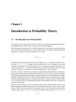
Chapter 1
Discrete Probability
Distributions
1.1 Simulation of Discrete Probabilities
Probability
In this chapter, we shall first consider chance experiments with a finite number of
possible outcomes ω
1
, ω
2

, . . . , ω
n
. For example, we roll a die and the possible
outcomes are 1, 2, 3, 4, 5, 6 corresponding to the side that turns up. We toss a coin
with possible outcomes H (heads) and T (tails).
It is frequently useful to be able to refer to an outcome of an experiment. For
example, we might want to write the mathematical expression which gives the sum
of four rolls of a die. To do this, we could let X
i
, i = 1, 2, 3, 4, represent the values
of the outcomes of the four rolls, and then we could write the expression
X
1
+ X
2
+ X
3
+ X
4
for the sum of the four rolls. The X
i
’s are called random variables. A random vari-
able is simply an expression whose value is the outcome of a particular experiment.
Just as in the case of other types of variables in mathematics, random variables can
take on different values.
Let X be the random variable which represents the roll of one die. We shall
assign probabilities to the possible outcome s of this experiment. We do this by
assigning to each outcome ω
j
a nonnegative number m(ω

j
) in such a way that
m(ω
1
) + m(ω
2
) + ···+ m(ω
6
) = 1 .
The function m(ω
j
) is called the distribution function of the random variable X.
For the case of the roll of the die we would assign equal probabilities or probabilities
1/6 to each of the outcomes. With this assignment of probabilities, one could write
P (X ≤ 4) =
2
3
1
2 CHAPTER 1. DISCRETE PROBABILITY DISTRIBUTIONS
to mean that the probability is 2/3 that a roll of a die will have a value which does
not exceed 4.
Let Y be the random variable which represents the toss of a coin. In this case,
there are two possible outcomes, which we can label as H and T. Unless we have
reason to suspect that the coin comes up one way more often than the other way,
it is natural to assign the probability of 1/2 to each of the two outcomes.
In both of the above experiments, each outcome is assigned an equal probability.
This would certainly not be the case in general. For example, if a drug is found to
be effective 30 percent of the time it is used, we might assign a probability .3 that
the drug is effective the next time it is used and .7 that it is not effective. This last
example illustrates the intuitive frequency concept of probability. That is, if we have

a probability p that an experiment will result in outcome A, then if we repeat this
experiment a large number of times we should expect that the fraction of times that
A will occur is about p. To check intuitive ideas like this, we shall find it helpful to
look at some of these problems experimentally. We could, for example, toss a coin
a large number of times and see if the fraction of times heads turns up is about 1/2.
We could also simulate this experiment on a computer.
Simulation
We want to be able to perform an experiment that corresponds to a given set of
probabilities; for example, m(ω
1
) = 1/2, m(ω
2
) = 1/3, and m(ω
3
) = 1/6. In this
case, one could mark three faces of a six-sided die with an ω
1
, two faces with an ω
2
,
and one face with an ω
3
.
In the general case we assume that m(ω
1
), m(ω
2
), . . . , m(ω
n
) are all rational

numbers, with least common denominator n. If n > 2, we can imagine a long
cylindrical die with a cross-section that is a regular n-gon. If m(ω
j
) = n
j
/n, then
we can label n
j
of the long faces of the cylinder with an ω
j
, and if one of the end
faces come s up, we can just roll the die again. If n = 2, a coin could be used to
perform the experiment.
We will be particularly interested in repeating a chance experiment a large num-
ber of times. Although the cylindrical die would be a convenient way to carry out
a few repetitions, it would be difficult to carry out a large number of experiments.
Since the modern computer can do a large numbe r of operations in a very short
time, it is natural to turn to the computer for this task.
Random Numbers
We must first find a computer analog of rolling a die. This is done on the computer
by means of a random number generator. Depending upon the particular software
package, the computer can be asked for a real number between 0 and 1, or an integer
in a given set of consecutive integers. In the first case, the real numbers are chosen
in such a way that the probability that the number lies in any particular subinterval
of this unit interval is equal to the length of the subinterval. In the second case,
each integer has the same probability of being chosen.
1.1. SIMULATION OF DISCRETE PROBABILITIES 3
.203309 .762057 .151121 .623868
.932052 .415178 .716719 .967412
.069664 .670982 .352320 .049723

.750216 .784810 .089734 .966730
.946708 .380365 .027381 .900794
Table 1.1: Sample output of the program RandomNumbers.
Let X be a random variable with distribution function m(ω), where ω is in the
set {ω
1
, ω
2
, ω
3
}, and m(ω
1
) = 1/2, m(ω
2
) = 1/3, and m(ω
3
) = 1/6. If our computer
package can return a random integer in the set {1, 2, , 6}, then we simply ask it
to do so, and make 1, 2, and 3 correspond to ω
1
, 4 and 5 correspond to ω
2
, and 6
correspond to ω
3
. If our computer package returns a random real numbe r r in the
interval (0, 1), then the expression
6r+ 1
will be a random integer between 1 and 6. (The notation x means the greatest
integer not exceeding x, and is read “floor of x.”)

The method by which random real numbers are generated on a computer is
described in the historical discussion at the end of this section. The following
example gives sample output of the program RandomNumbers.
Example 1.1 (Random Number Generation) The program RandomNumbers
generates n random real numbe rs in the interval [0, 1], where n is chosen by the
user. When we ran the program with n = 20, we obtained the data shown in
Table 1.1. ✷
Example 1.2 (Coin Tossing) As we have noted, our intuition suggests that the
probability of obtaining a head on a single toss of a c oin is 1/2. To have the
computer toss a coin, we can ask it to pick a random real number in the interval
[0, 1] and test to see if this number is less than 1/2. If so, we shall call the outcome
heads; if not we call it tails. Another way to proceed would be to ask the computer
to pick a random integer from the set {0, 1}. The program CoinTosses carries
out the experiment of tossing a coin n times. Running this program, with n = 20,
resulted in:
THTTTHTTTTHTTTTTHHTT.
Note that in 20 tosses, we obtained 5 heads and 15 tails. Let us toss a coin n
times, where n is much larger than 20, and see if we obtain a proportion of heads
closer to our intuitive guess of 1/2. The program CoinTosses keeps track of the
number of heads. When we ran this program with n = 1000, we obtained 494 heads.
When we ran it with n = 10000, we obtained 5039 heads.
4 CHAPTER 1. DISCRETE PROBABILITY DISTRIBUTIONS
We notice that when we tossed the coin 10,000 times, the proportion of heads
was close to the “true value” .5 for obtaining a head when a coin is tossed. A math-
ematical mo del for this experiment is called Bernoulli Trials (see Chapter 3). The
Law of Large Numbers, which we shall study later (see Chapter 8), will show that
in the Bernoulli Trials model, the prop ortion of heads should be near .5, consistent
with our intuitive idea of the frequency interpretation of probability.
Of course, our program could be easily modified to simulate coins for which the
probability of a head is p, where p is a real number between 0 and 1. ✷

In the case of coin tossing, we already knew the probability of the event o cc urring
on each experiment. The real power of simulation comes from the ability to estimate
probabilities when they are not known ahead of time. This method has been used in
the recent discoveries of strategies that make the casino game of blackjack favorable
to the player. We illustrate this idea in a simple situation in which we can compute
the true probability and see how effective the simulation is.
Example 1.3 (Dice Rolling) We consider a dice game that played an important
role in the historical development of probability. The famous letters between Pas-
cal and Fermat, which many believe started a serious study of probability, were
instigated by a request for help from a French nobleman and gambler, Chevalier
de M´er´e. It is said that de M´er´e had been betting that, in four rolls of a die, at
least one six would turn up. He was winning consistently and, to get more people
to play, he changed the game to bet that, in 24 rolls of two dice, a pair of sixes
would turn up. It is claimed that de M´er´e lost with 24 and felt that 25 rolls were
necessary to make the game favorable. It was un grand scandale that mathematics
was wrong.
We shall try to see if de M´er´e is correct by simulating his various bets. The
program DeMere1 simulates a large number of experiments, seeing, in each one,
if a six turns up in four rolls of a die. When we ran this program for 1000 plays,
a six came up in the first four rolls 48.6 percent of the time. When we ran it for
10,000 plays this happened 51.98 percent of the time.
We note that the result of the s ec ond run s uggests that de M´er´e was correct
in believing that his bet with one die was favorable; howe ver, if we had based our
conclusion on the first run, we would have decided that he was wrong. Accurate
results by simulation require a large number of experiments. ✷
The program DeMere2 simulates de M´er´e’s second bet that a pair of sixes
will occur in n rolls of a pair of dice. The previous simulation shows that it is
important to know how many trials we should simulate in order to expect a certain
degree of accuracy in our approximation. We shall see later that in these types of
experiments, a rough rule of thumb is that, at least 95% of the time, the error does

not exceed the reciprocal of the square root of the number of trials. Fortunately,
for this dice game, it will be easy to compute the exact probabilities. We s hall
show in the next s ec tion that for the first bet the probability that de M´er´e wins is
1 −(5/6)
4
= .518.
1.1. SIMULATION OF DISCRETE PROBABILITIES 5
5
10 15 20 25 30 35 40
-10
-8
-6
-4
-2
2
4
6
8
10
Figure 1.1: Peter’s winnings in 40 plays of heads or tails.
One can understand this calculation as follows: The probability that no 6 turns
up on the first toss is (5/6). The probability that no 6 turns up on either of the
first two tosses is (5/6)
2
. Reasoning in the same way, the probability that no 6
turns up on any of the first four tosses is (5/6)
4
. Thus, the probability of at least
one 6 in the first four tosses is 1 − (5/6)
4

. Similarly, for the second bet, with 24
rolls, the probability that de M´er´e wins is 1 − (35/36)
24
= .491, and for 25 rolls it
is 1 − (35/36)
25
= .506.
Using the rule of thumb mentioned above, it would require 27,000 rolls to have a
reasonable chance to determine these probabilities with sufficient accuracy to assert
that they lie on opposite sides of .5. It is interesting to p onder whether a gambler
can detect such probabilities with the required accuracy from gambling experience.
Some writers on the history of probability suggest that de M´er´e was, in fact, just
interested in these problems as intriguing probability problems.
Example 1.4 (Heads or Tails) For our next example, we consider a problem where
the exact answer is difficult to obtain but for which simulation easily gives the
qualitative results. Peter and Paul play a game called heads or tails. In this game,
a fair coin is tossed a sequence of times—we choose 40. Each time a head comes up
Peter wins 1 penny from Paul, and each time a tail comes up Peter loses 1 penny
to Paul. For example, if the results of the 40 tosses are
THTHHHHTTHTHHTTHHTTTTHHHTHHTHHHTHHHTTTHH.
Peter’s winnings may be graphed as in Figure 1.1.
Peter has won 6 pennies in this particular game . It is natural to ask for the
probability that he will win j pennies; here j could be any even number from −40
to 40. It is reasonable to guess that the value of j with the highest probability
is j = 0, since this occurs when the number of heads equals the number of tails.
Similarly, we would guess that the values of j with the lowest probabilities are
j = ±40.
6 CHAPTER 1. DISCRETE PROBABILITY DISTRIBUTIONS
A second interesting question about this game is the following: How many times
in the 40 tosses will Peter be in the lead? Looking at the graph of his winnings

(Figure 1.1), we see that Peter is in the lead when his winnings are positive, but
we have to make some convention when his winnings are 0 if we want all tosses to
contribute to the number of times in the lead. We adopt the convention that, when
Peter’s winnings are 0, he is in the lead if he was ahead at the previous toss and
not if he was behind at the previous toss. With this convention, Peter is in the lead
34 times in our example. Again, our intuition might suggest that the most likely
number of times to be in the lead is 1/2 of 40, or 20, and the least likely numbers
are the extreme cases of 40 or 0.
It is easy to settle this by simulating the game a large number of times and
keeping track of the number of times that Peter’s final winnings are j, and the
number of times that Peter ends up being in the lead by k. The proportions over
all games then give estimates for the corresponding probabilities. The program
HTSimulation carries out this simulation. Note that when there are an even
number of tos se s in the game, it is possible to be in the lead only an even number
of times. We have simulated this game 10,000 times. The results are shown in
Figures 1.2 and 1.3. These graphs, which we call spike graphs, were generated
using the program Spikegraph. The vertical line, or spike, at position x on the
horizontal axis, has a height equal to the proportion of outcomes which equal x.
Our intuition about Peter’s final winnings was quite correct, but our intuition about
the number of times Peter was in the lead was completely wrong. The simulation
suggests that the least likely number of times in the lead is 20 and the most likely
is 0 or 40. This is indeed correct, and the explanation for it is suggested by playing
the game of heads or tails with a large number of tosses and looking at a graph of
Peter’s winnings. In Figure 1.4 we show the results of a simulation of the game, for
1000 tosses and in Figure 1.5 for 10,000 tosses.
In the second example Peter was ahead mos t of the time. It is a remarkable
fact, however, that, if play is c ontinued long enough, Peter’s winnings will continue
to come back to 0, but there will be very long times between the times that this
happ e ns. These and related results will be discussed in Chapter 12. ✷
In all of our examples so far, we have simulated equiprobable outcomes. We

illustrate next an example where the outcomes are not equiprobable.
Example 1.5 (Horse Races) Four horses (Acorn, Balky, Chestnut, and Dolby)
have raced many times. It is e stimated that Acorn wins 30 percent of the time,
Balky 40 percent of the time, Chestnut 20 percent of the time, and Dolby 10 percent
of the time.
We can have our computer carry out one race as follows: Choose a random
number x. If x < .3 then we say that Acorn won. If .3 ≤ x < .7 then Balky wins.
If .7 ≤ x < .9 then Chestnut wins. Finally, if .9 ≤ x then Dolby wins.
The program HorseRace uses this method to simulate the outcomes of n races.
Running this program for n = 10 we found that Acorn won 40 percent of the time,
Balky 20 percent of the time, Chestnut 10 percent of the time, and Dolby 30 percent
1.1. SIMULATION OF DISCRETE PROBABILITIES 7
Figure 1.2: Distribution of winnings.
Figure 1.3: Distribution of number of times in the lead.
8 CHAPTER 1. DISCRETE PROBABILITY DISTRIBUTIONS
200 400 600 800 1000
1000 plays
-50
-40
-30
-20
-10
0
10
20
Figure 1.4: Peter’s winnings in 1000 plays of heads or tails.
2000 4000 6000 8000 10000
10000 plays
0
50

100
150
200
Figure 1.5: Peter’s winnings in 10,000 plays of heads or tails.
1.1. SIMULATION OF DISCRETE PROBABILITIES 9
of the time. A larger number of race s would be necessary to have better agreem ent
with the past experience. Therefore we ran the program to simulate 1000 races
with our four horses. Although very tired after all these races, they performed in
a manner quite consistent with our estimates of their abilities. Acorn won 29.8
percent of the time, Balky 39.4 percent, Chestnut 19.5 perce nt, and Dolby 11.3
percent of the time.
The program GeneralSimulation uses this method to simulate repetitions of
an arbitrary experiment with a finite number of outcomes occurring with known
probabilities. ✷
Historical Remarks
Anyone who plays the same chance game over and over is really carrying out a sim-
ulation, and in this sense the process of simulation has been going on for centuries.
As we have remarked, many of the early problems of probability might well have
been suggested by gamblers’ exp eriences .
It is natural for anyone trying to understand probability theory to try simple
experiments by tossing coins, rolling dice, and so forth. T he naturalist Buffon tossed
a coin 4040 times , resulting in 2048 heads and 1992 tails. He also estimated the
number π by throwing needles on a ruled surface and recording how many times
the needles crossed a line (see Section 2.1). The English biologist W. F. R. Weldon
1
recorded 26,306 throws of 12 dice, and the Swiss scientist Rudolf Wolf
2
recorded
100,000 throws of a single die without a computer. Such experiments are very time-
consuming and may not accurately represent the chance phenomena being studied.

For example, for the dice experiments of Weldon and Wolf, further analysis of the
recorded data showed a suspected bias in the dice. The statistician Karl Pearson
analyzed a large number of outcomes at certain roulette tables and suggested that
the wheels were biased. He wrote in 1894:
Clearly, since the Casino does not serve the valuable end of huge lab-
oratory for the preparation of probability statistics, it has no scientific
raison d’ˆetre. Men of sc ience cannot have their most refined theories
disregarded in this shameless manner! The French Government must be
urged by the hierarchy of science to close the gaming-saloons; it would
be, of course, a graceful act to hand over the remaining resources of the
Casino to the Acad´emie des Sciences for the endowment of a laboratory
of orthodox probability; in particular, of the new branch of that study,
the application of the theory of chance to the biological problems of
evolution, which is likely to occupy so much of men’s thoughts in the
near future.
3
However, these early experiments were suggestive and led to important discov-
eries in probability and statistics. They led Pearson to the chi-squared test, which
1
T. C. Fry, Probability and Its Engineering Uses, 2nd ed. (Princeton: Van Nostrand, 1965).
2
E. Czuber, Wahrscheinlichkeitsrechnung, 3rd ed. (Berlin: Teubner, 1914).
3
K. Pearson, “Science and Monte Carlo,” Fortnightly Review, vol. 55 (1894), p. 193; cited in
S. M. Stigler, The History of Statistics (Cambridge: Harvard University Press, 1986).
10 CHAPTER 1. DISCRETE PROBABILITY DISTRIBUTIONS
is of great importance in testing whether observed data fit a given probability dis-
tribution.
By the early 1900s it was clear that a better way to generate random numbers
was needed. In 1927, L. H. C. Tippett published a list of 41,600 digits obtained by

selecting numbers haphazardly from census reports. In 1955, RAND Corporation
printed a table of 1,000,000 random numbers generated from electronic noise. The
advent of the high-speed computer raised the possibility of generating random num-
bers directly on the computer, and in the late 1940s John von Neumann suggested
that this be done as follows: Suppose that you want a random sequence of four-digit
numbers. Choose any four-digit number, say 6235, to start. Square this number
to obtain 38,875,225. For the second number choose the middle four digits of this
square (i.e., 8752). Do the same process starting with 8752 to get the third number,
and so forth.
More modern methods involve the concept of modular arithmetic. If a is an
integer and m is a positive integer, then by a (mod m) we mean the remainder
when a is divided by m. For example, 10 (mod 4) = 2, 8 (mod 2) = 0, and so
forth. To generate a random sequence X
0
, X
1
, X
2
, . . . of numbers choose a starting
number X
0
and then obtain the numbers X
n+1
from X
n
by the formula
X
n+1
= (aX
n

+ c) (mod m) ,
where a, c, and m are carefully chosen constants. The sequence X
0
, X
1
, X
2
, . . .
is then a sequence of integers between 0 and m − 1. To obtain a sequence of real
numbers in [0, 1), we divide each X
j
by m. The resulting sequence consists of
rational numbers of the form j/m, where 0 ≤ j ≤ m − 1. Since m is usually a
very large integer, we think of the numbers in the sequence as b e ing random real
numbers in [0, 1).
For both von Neumann’s squaring method and the modular arithmetic technique
the sequence of numbers is actually completely determined by the first number.
Thus, there is nothing really random about these sequences. However, they produce
numbers that behave very much as theory would predict for random experiments.
To obtain different sequences for different experiments the initial number X
0
is
chosen by some other procedure that might involve, for example, the time of day.
4
During the Second World War, physicists at the Los Alamos Scientific Labo-
ratory needed to know, for purposes of shielding, how far neutrons travel through
various materials. This question was beyond the reach of theoretical calculations.
Daniel McCracken, writing in the Scientific American, states:
The physicists had most of the necessary data: they knew the average
distance a neutron of a given speed would travel in a given substance

before it collided with an atomic nucleus, what the probabilities were
that the neutron would bounce off instead of being absorbed by the
nucleus, how much energy the neutron was likely to lose after a given
4
For a detailed discussion of random numbers, see D. E. Knuth, The Art of Computer Pro-
gramming, vol. II (Reading: Addison-Wesley, 1969).
1.1. SIMULATION OF DISCRETE PROBABILITIES 11
collision and so on.
5
John von Neumann and Stanislas Ulam suggested that the problem be solved
by modeling the experiment by chance devices on a computer. Their work being
secret, it was necessary to give it a code name. Von Neumann chose the name
“Monte Carlo.” Since that time, this method of simulation has been called the
Monte Carlo Method.
William Feller indicated the possibilities of using computer simulations to illus-
trate basic concepts in probability in his book An Introduction to Probability Theory
and Its Applications. In discussing the problem about the number of times in the
lead in the game of “heads or tails” Feller writes:
The results concerning fluctuations in coin tossing show that widely
held beliefs about the law of large numbers are fallacious. These results
are so amazing and so at variance with common intuition that even
sophisticated colleagues doubted that coins actually misbehave as theory
predicts. The record of a simulated experiment is therefore included.
6
Feller provides a plot showing the result of 10,000 plays of heads or tails similar to
that in Figure 1.5.
The martingale betting system described in Exercise 10 has a long and interest-
ing history. Russell Barnhart pointed out to the authors that its use can be traced
back at least to 1754, when Casanova, writing in his memoirs, History of My Life,
writes

She [Casanova’s mistress] made me promise to go to the casino [the
Ridotto in Venice] for money to play in partnership with her. I went
there and took all the gold I found, and, determinedly doubling my
stakes acc ording to the system known as the martingale, I won three or
four times a day during the rest of the Carnival. I never lost the sixth
card. If I had lost it, I should have been out of funds, which amounted
to two thousand zecchini.
7
Even if there were no zeros on the roulette wheel so the game was perfectly fair,
the martingale system, or any other system for that matter, cannot make the game
into a favorable game. The idea that a fair game remains fair and unfair games
remain unfair under gambling systems has been exploited by mathematicians to
obtain important results in the study of probability. We will introduce the general
concept of a martingale in Chapter 6.
The word martingale itself also has an interesting history. The origin of the
word is obscure. A recent version of the Oxford English Dictionary gives examples
5
D. D. McCracken, “The Monte Carlo Method,” Scientific American, vol. 192 (May 1955),
p. 90.
6
W. Feller, Introduction to Probability Theory and its Applications, vol. 1, 3rd ed. (New York:
John Wiley & Sons, 1968), p. xi.
7
G. Casanova, History of My Life, vol. IV, Chap. 7, trans. W. R. Trask (New York: Harcourt-
Brace, 1968), p. 124.
12 CHAPTER 1. DISCRETE PROBABILITY DISTRIBUTIONS
of its use in the early 1600s and says that its probable origin is the reference in
Rabelais’s Book One, Chapter 20:
Everything was done as planned, the only thing being that Gargantua
doubted if they would be able to find, right away, breeches suitable to

the old fellow’s legs; he was doubtful, also, as to what cut would be most
becoming to the orator—the martingale, which has a draw-bridge effect
in the seat, to permit doing one’s business more easily; the sailor-style,
which affords more comfort for the kidneys; the Swiss, which is warmer
on the belly; or the codfish-tail, which is cooler on the loins.
8
Dominic Lusinchi noted an earlier occurrence of the word martingale. Accord-
ing to the French dictionary Le Petit Robert, the word comes from the Proven¸cal
word “martegalo,” which means “from Martigues.” Martigues is a town due west of
Merseille. The dictionary give s the example of “chausses `a la martinguale” (which
means Martigues-style breeches ) and the date 1491.
In modern uses martingale has several different meanings, all related to holding
down, in addition to the gambling use. For example, it is a strap on a horse’s
harness used to hold down the horse’s head, and also part of a sailing rig used to
hold down the bowsprit.
The Labouchere system described in Exercise 9 is named after Henry du Pre
Labouchere (1831–1912), an English journalist and member of Parliament. Labou-
chere attributed the system to Condorcet. Condorcet (1743–1794) was a political
leader during the time of the French revolution who was interested in applying prob-
ability theory to economics and politics. For example, he calculated the probability
that a jury using majority vote will give a correct decision if each juror has the
same probability of deciding correctly. His writings provided a wealth of ideas on
how probability might be applied to human affairs.
9
Exercises
1 Modify the program CoinTosses to toss a coin n times and print out after
every 100 tosses the proportion of heads minus 1/2. Do these numbers appear
to approach 0 as n increases? Modify the program again to print out, every
100 times, both of the following quantities: the proportion of heads minus 1/2,
and the number of heads minus half the number of tosses. Do these numbers

appear to approach 0 as n increases?
2 Modify the program CoinTosses so that it tosses a coin n times and records
whether or not the proportion of heads is within .1 of .5 (i.e., between .4
and .6). Have your program repeat this experiment 100 times. About how
large must n be so that approximately 95 out of 100 times the proportion of
heads is between .4 and .6?
8
Quoted in the Portable Rabelais, ed. S. Putnam (New York: Viking, 1946), p. 113.
9
Le Marquise de Condorcet, Essai sur l’Application de l’Analyse `a la Probabilit´e d`es D´ecisions
Rendues a la Pluralit´e des Voix (Paris: Imprimerie Royale, 1785).
1.1. SIMULATION OF DISCRETE PROBABILITIES 13
3 In the early 1600s, Galileo was asked to explain the fact that, although the
number of triples of integers from 1 to 6 with sum 9 is the same as the number
of such triples with sum 10, when three dice are rolled, a 9 seemed to come
up less often than a 10—supposedly in the experience of gamblers.
(a) Write a program to simulate the roll of three dice a large number of
times and keep track of the proportion of times that the sum is 9 and
the proportion of times it is 10.
(b) Can you conclude from your simulations that the gamblers were correct?
4 In raquetball, a player continues to serve as long as she is winning; a point
is scored only when a player is serving and wins the volley. The first player
to win 21 points wins the game. Assume that you serve first and have a
probability .6 of winning a volley when you serve and probability .5 when
your opponent serves. Estimate, by simulation, the probability that you will
win a game.
5 Consider the bet that all three dice will turn up sixes at least once in n rolls
of three dice. Calculate f(n), the probability of at least one triple-six when
three dice are rolled n times. Determine the smallest value of n necessary for
a favorable bet that a triple-six will occur when three dice are rolled n times.

(DeMoivre would say it should be about 216 log 2 = 149.7 and so would answer
150—see Exercise 1.2.17. Do you agree with him?)
6 In Las Vegas, a roulette wheel has 38 slots numbered 0, 00, 1, 2, . . . , 36. The
0 and 00 slots are green and half of the remaining 36 slots are red and half
are black. A croupier spins the wheel and throws in an ivory ball. If you bet
1 dollar on red, you win 1 dollar if the ball stops in a red slot and otherwise
you lose 1 dollar. Write a program to find the total winnings for a player who
makes 1000 bets on red.
7 Another form of bet for roulette is to bet that a specific number (say 17) will
turn up. If the ball stops on your number, you get your dollar back plus 35
dollars. If not, you lose your dollar. Write a program that will plot your
winnings when you make 500 plays of roulette at Las Vegas, first when you
bet each time on red (see Exercise 6), and then for a second visit to Las
Vegas when you make 500 plays betting each time on the number 17. What
differences do you see in the graphs of your winnings on these two occasions?
8 An astute student noticed that, in our simulation of the game of heads or tails
(see Example 1.4), the proportion of times the player is always in the lead is
very close to the prop ortion of times that the player’s total winnings end up 0.
Work out these probabilities by enumeration of all cases for two tosses and
for four tosses, and see if you think that these probabilities are, in fact, the
same.
9 The Labouchere system for roulette is played as follows. Write down a list of
numbers, usually 1, 2, 3, 4. Bet the sum of the first and last, 1 + 4 = 5, on
14 CHAPTER 1. DISCRETE PROBABILITY DISTRIBUTIONS
red. If you win, delete the first and last numbers from your list. If you lose,
add the amount that you last bet to the end of your list. Then use the new
list and bet the sum of the first and last numbers (if there is only one number,
bet that amount). Continue until your list becomes empty. Show that, if this
happ e ns, you win the sum, 1 + 2 + 3 + 4 = 10, of your original list. Simulate
this system and see if you do always stop and, hence, always win. If so, why

is this not a foolproof gambling system?
10 Another well-known gambling system is the martingale doubling system. Sup-
pose that you are betting on red to turn up in roulette. Every time you win,
bet 1 dollar next time. Every time you lose, double your previous bet. Suppose
that you use this system until you have won at least 5 dollars or you have lost
more than 100 dollars. Write a program to simulate this and play it a number
of times and see how you do. In his book The Newcomes, W. M. Thack-
eray remarks “You have not played as yet? Do not do s o; above all avoid a
martingale if you do.”
10
Was this good advice?
11 Modify the program HTSimulation so that it keeps track of the maximum of
Peter’s winnings in each game of 40 tosses. Have your program print out the
prop ortion of times that your total winnings take on values 0, 2, 4, . . . , 40.
Calculate the corresponding exact probabilities for games of two tosses and
four tosses.
12 In an upcoming national election for the President of the United States, a
pollster plans to predict the winner of the p opular vote by taking a random
sample of 1000 voters and declaring that the winner will be the one obtaining
the most votes in his sample. Suppose that 48 pe rcent of the voters plan
to vote for the Republican candidate and 52 percent plan to vote for the
Democratic candidate. To get some idea of how reasonable the pollster’s
plan is, write a program to make this prediction by simulation. Repeat the
simulation 100 times and see how many times the pollster’s prediction would
come true. Repeat your experiment, assuming now that 49 percent of the
population plan to vote for the Republican candidate; first with a sample of
1000 and then with a sample of 3000. (The Gallup Poll uses about 3000.)
(This idea is discussed further in Chapter 9, Section 9.1.)
13 The psychologist Tversky and his colleagues
11

say that about four out of five
people will answer (a) to the following question:
A certain town is served by two hospitals. In the larger hospital about 45
babies are born each day, and in the smaller hospital 15 babies are born each
day. Although the overall proportion of boys is about 50 percent, the actual
prop ortion at either hospital may be more or less than 50 percent on any day.
10
W. M. Thackerey, The Newcomes (London: Bradbury and Evans, 1854–55).
11
See K. McKean, “Decisions, Decisions,” Discover, June 1985, pp . 22–31. Kevin McKean,
Discover Magazine,
c
1987 Famil y Media, Inc. Reprinted with permission. This popular article
reports on the work of Tverksy et. al. in Judgement Under Uncertainty: Heuristics and Biases
(Cambridge: Cambridge University Press, 1982).
1.1. SIMULATION OF DISCRETE PROBABILITIES 15
At the end of a year, which hospital will have the greater number of days on
which more than 60 percent of the babies born were boys?
(a) the large hospital
(b) the small hospital
(c) neither—the number of days will be about the same.
Assume that the probability that a baby is a boy is .5 (actual estimates make
this more like .513). Decide, by simulation, what the right answer is to the
question. Can you suggest why so many people go wrong?
14 You are offered the following game. A fair coin will be tossed until the first
time it comes up heads. If this occurs on the jth toss you are paid 2
j
dollars.
You are sure to win at least 2 dollars so you should be willing to pay to play
this game—but how much? Few people would pay as much as 10 dollars to

play this game. See if you can decide, by simulation, a reasonable amount
that you would be willing to pay, per game, if you will be allowed to make
a large number of plays of the game. Does the amount that you would be
willing to pay per game depend upon the number of plays that you will be
allowed?
15 Tversky and his colleagues
12
studied the records of 48 of the Philadelphia
76ers basketball games in the 1980–81 season to see if a player had times
when he was hot and every shot went in, and other times when he was cold
and barely able to hit the backboard. The players estimated that they were
about 25 percent more likely to make a shot after a hit than after a miss.
In fact, the opposite was true—the 76ers were 6 percent more likely to score
after a miss than after a hit. Tversky reports that the number of hot and cold
streaks was about what one would expect by purely random effects. Assuming
that a player has a fifty-fifty chance of making a shot and makes 20 shots a
game, estimate by simulation the proportion of the games in which the player
will have a streak of 5 or more hits.
16 Estimate, by simulation, the average number of children there would be in
a family if all people had children until they had a boy. Do the same if all
people had children until they had at least one boy and at least one girl. How
many more children would you expect to find under the second scheme than
under the first in 100,000 families? (Assume that boys and girls are equally
likely.)
17 Mathematicians have been known to get some of the best ideas while sitting in
a cafe, riding on a bus, or strolling in the park. In the early 1900s the famous
mathematician George P´olya lived in a hotel near the woods in Zurich. He
liked to walk in the woods and think about mathematics. P´olya describes the
following incident:
12

ibid.