Is there Room for Forex Interventions under Inflation Targeting Framework? Evidence from Mexico and Turkey pptx
Bạn đang xem bản rút gọn của tài liệu. Xem và tải ngay bản đầy đủ của tài liệu tại đây (646.12 KB, 33 trang )
Is there Room for Forex Interventions under Inflation Targeting Framework?
Evidence from Mexico and Turkey
by
Ilker Domaç
†
and Alfonso Mendoza
‡
Abstract
The salient characteristics of emerging market economies coupled with the increasing
adoption of inflation targeting (IT) in these countries has stimulated much debate about
the role of the exchange rate in IT regimes. The paper aims at shedding more light on this
issue by investigating whether central bank foreign exchange interventions have any
impact on the volatility of the exchange rate in Mexico and Turkey since the adoption of
the floating regime. To this end, the study, using daily data on foreign exchange
intervention, employs an Exponential GARCH framework. Empirical results suggest that
both the amount and frequency of foreign exchange interventions have decreased the
volatility of the exchange rates in these countries. The findings corroborate the notion
that if foreign exchange interventions are carried out with finesse and sensibly—i.e., not
to defend a particular exchange rate—they could play a useful role under IT framework
in containing the adverse effects of temporary exchange rate shocks on inflation and
financial stability.
Keywords: Inflation targeting; exchange rate volatility; central bank intervention; E-GARCH.
JEL classification: C32; E58; F31; G15
The views expressed in this paper are those of the authors and should not be attributed to the institutions
with which they are affiliated.
† Corresponding author.
Central Bank of Turkey
Istiklal Caddesi No:10
Ulus, Ankara 06100
Turkey
E-mail Address:
‡ The University of York
E-mail Address:
1. Introduction
The successful performance of a number of industrialized countries that adopted
inflation targeting (IT) has rendered this monetary policy strategy an attractive
alternative for emerging market economies (EMs). Indeed, a number of EMs has already
instituted IT or some form of this monetary policy framework. The increasing attraction
of inflation targeting among EMs as a monetary policy framework combined with the
salient characteristics of EMs has, in turn, stimulated much discussion about the role of
exchange rate in inflation targeting regimes.
More specifically, it is argued that emerging market economies are often beset by
a lack of credibility and limited access to international markets; they are beset by more
pronounced adverse effects of exchange rate volatility on trade, high liability
dollarization, and higher pass-through from the exchange rate to inflation.
1
Consequently, it is argued that benign neglect of the exchange rate is not a feasible option
for emerging market economies.
This, in turn, begs the following question: How should policy makers take
account of the exchange rate under IT? It is true that under IT, the credibility of the
regime entails an institutional commitment to price stability as the primary goal of
monetary policy, to which other goals, including the exchange rate, are subordinated.
Monetary authorities in EMs, however, may need to take exchange rate movements into
consideration at least for two reasons. First, the evolution of the exchange rate has an
important impact on inflation owing to the open nature of EMs. Second, the presence of
a thin foreign exchange market or temporary shocks in EMs often forces these countries
to dampen short-term exchange rate volatility.
1
Calvo (1999).
2
As a consequence, EMs often resort to intervening or adjusting interest rates to
contain the effect of temporary exchange rate shocks on inflation and financial stability.
2
In practice, it appears that all inflation targeting central banks explicitly allow for the
option of intervening in foreign exchange markets, although industrial countries have
rarely relied on this option in recent years (see Appendix). Indeed, evidence suggests that
EMs, which typically have thinly-traded securities, engaged in foreign exchange
interventions more frequently compared to industrial countries since they are more
vulnerable to disturbances stemming from the foreign exchange market (Carere et. al.
(2002)).
Responding too heavily and too frequently to movements in the exchange rate
under IT, however, runs the risk of transforming the exchange rate into a nominal anchor
for monetary policy that takes precedence over the inflation target. One possible way to
avoid this problem for inflation targeting central banks in EMs is to adopt transparent
mechanisms which would ensure that polices to influence the exchange rate are aimed at
smoothing the impact of temporary shocks and achieving the inflation objective.
Granted that central banks adopt such mechanisms, can they really mitigate
unwarranted short-run exchange rate fluctuations? In the context of the IT framework,
this study aims to shed more light on this issue by considering the experiences of Mexico
and Turkey under the floating regime. To this end, the paper attempts to model central
bank intervention and its effect on volatility with autoregressive conditional
heteroscedasticity models. In particular, the study employs the Exponential-GARCH
model of Nelson (1991), which allows for the inclusion of negative values as exogenous
2
See Goldstein (2001) and Mishkin and Schmidt-Hebbel (2001) for more on this.
3
shocks in the variance, with a view to study the impact of sale and purchase operations
separately in the analysis.
The empirical findings suggest that both the amount and frequency of foreign
exchange interventions have decreased the volatility of the exchange rates in countries
under consideration. The results imply that sale operations are effective in influencing
the exchange rate and its volatility, while purchase operations are found to be statistically
insignificant in affecting the exchange rate and its volatility. All in all, the findings lend
support to the notion that if foreign exchange interventions are carried out with finesse
and sensibly—i.e., not to defend a particular exchange rate—they could play a useful role
under IT framework in mitigating the adverse effects of temporary exchange rate shocks
on inflation and financial stability.
The remainder of this paper is organized as follows. The next section provides a
brief overview of the literature on central bank intervention. Section 3 discusses the key
aspects of the intervention mechanisms in Mexico and Turkey under floating exchange
rate regime. Section 4 describes the empirical framework to model conditional volatility
and the effect of central bank interventions. Section 5 presents the empirical results.
Section 6 concludes the paper.
2. A Brief Review of the Literature on Central Bank Intervention
This section briefly reviews the literature on central bank intervention. Empirical
studies and the statements by central banks suggest that central banks intervene in foreign
exchange markets to slow or correct excessive trends in the exchange rate, i.e. they “lean
against the wind”, and to calm disorderly markets (Lewis 1995, Baille and Osterberg
4
1997). The channels through which a non-sterilized intervention in the foreign market
may affect the exchange rate are well known in the economic literature.
3
A purchase of
dollars from the Central Bank may depreciate the underlying currency in the same
proportion to the increase in liquidity on the money market and vice versa.
Sterilized intervention, on the other hand, might affect the exchange rate not
through changes in liquidity, but through two main channels: portfolio balance channel
and the signaling channel. The portfolio balance channel assumes that investors diversify
based on mean variance analysis.
4
As long as foreign and domestic bonds are imperfect
substitutes, sterilized interventions, which alter the relative supply of local bonds, will
always induce a change in the composition of the investor’s portfolio. Investors will then
require a greater (lower) return—measured by a risk premium—to absorb the increased
(lower) supply of such instruments and this, along with an equal-amount-increase in the
demand for foreign bonds, will cause a depreciation (appreciation) of the exchange rate.
Since interventions are small relative to the stock of outstanding bonds most
authors, including Rogoff (1984), have expressed skepticism that interventions could
have large impact through the portfolio balance channel. Not surprisingly, many studies
do not find evidence of this channel and those that do such as Evans and Lyons (2001)
and Ghosh (1992) suggest it is weak.
The signaling channel refers to the signals sent by the central bank to the market.
More specifically, if the central bank uses foreign exchange interventions credibly to
indicate intended changes in monetary policy, the resulting appreciation of the exchange
3
For a more thorough review of the literature see Sarno and Taylor (2001), Dominguez and Frankel
(1993b), and Edison (1993).
4
A detailed analysis and description of the portfolio effect can be found in Domínguez and Frenkel
(1993a).
5
rate can be described as the signaling channel. The policy intentions or beliefs of the
authority with respect to the foreign exchange market are made explicit with the aim of
stabilizing or re-directing the market. Even in the case where such intentions are never
realized, the exchange rate may change as a result of changing expectations about
fundamentals.
The impact of intervention through the signaling channel has often been found to
be substantially stronger than through the portfolio balance channel (Dominguez and
Frankel (1993a)). For the signaling channel to be an ongoing transmission mechanism,
central banks should be seen to follow interventions with appropriate changes in
monetary policy. Consequently, interventions operating through the signaling channel do
not constitute an independent policy tool.
5
3. A Quick Glance at the key Aspects of Foreign Exchange Intervention Policies in
Mexico and Turkey
3.1 The Banco de México
In the face of balance of payments and financial crisis, the Central Bank could no
longer defend the predetermined parity and decided to float the peso on December 19
th
1994. With the adoption of the floating regime, the management of monetary aggregates
became the anchor for the evolution of the general price level by early 1995. During the
first half of 1995, however, the authorities modified this ruled based strategy centered
solely on quantitative targets by incorporating discretion (via influencing the level of
5
A recent study on Mexico, which aimed at investigating the portfolio and signaling effect, indicated that
dollar purchases through the options mechanism have not significantly affected the foreign exchange
market (Werner (1997b)).
6
interest rates) in the conduct of monetary policy. Under the new strategy, the discretion
was constrained by the following ultimate goal: the attainment of the annual inflation
objective, and in the medium to long run, the gradual reduction of inflation. This
framework was maintained until 1997 and thereafter the monetary policy framework
began a gradual transition toward an explicit full-fledged inflation targeting regime. As a
consequence, the monetary base became less relevant and the inflation target more
significant in the implementation of monetary policy. The Central Bank announced a
series of annual inflation targets in 1999 with a view to converge to the inflation rate
prevailing in the country’s main trading partners. From this year on, the actual annual
rates of inflation have been below their ceilings and the Central Bank expects to attain its
final goal of a stationary annual inflation target of 3 percent by 2003.
6
Although it is no longer the anchor of the economy, the role of the exchange rate
as an adjustment variable in the conduct of the monetary policy still remains crucial. The
intensity of pass-trough shocks on inflation and output levels (and volatility) hinge on the
relative stability of the exchange rate, which, by and large, lies behind the policies of
sterilized foreign exchange rate intervention. Such stabilization has presumably relied
more on the effectiveness of USD sales in the foreign exchange market than to USD
purchases, which have been mainly utilized to increase the amount of international assets.
In August 1996, the authorities decided to auction Put Options
7
on the last
business day of each month, giving the right to credit institutions of selling dollars to the
Banco de México in any day during the life of the contract as long as the exercise price
6
See Schmidt-Hebbel and Werner (2002) for more on this.
7
This section provides a brief description of the derivatives mechanism. A more comprehensive discussion
of this issue can be found in Werner and Milo (1998).
7
(determined a day earlier) is no greater than the twenty-day moving average of the ‘fix
exchange rate’.
8
Figure 1 presents the cumulative net purchases of USD since August 1996. By the
end of the Put Options program in June 2001, international reserves represented a 30% of
the 40,866 millions of dollars. In total, market conditions allowed the participants to
exercise the derivative instruments 132 times. Although there is no a clear policy of
international reserves holdings, from the authorities’ standpoint, this amount of foreign
currency seems to be sufficient to insure the floating of the peso against capital flight or
sudden shocks to the capital account.
Figure 1. Banco de Mexico’s cumulative purchases of dollars
a
Figure 2. Daily purchases and sales of US dollars
b
0 2000 4000 6000 8000 10000 12000
8/1/1996 4/1/1997 12/1/1997 8/1/1998 4/1/1999 12/1/1999 8/1/2000 4/1/2001
$US millions
-400 -100 200 500
01.08.96 01.03.97 01.10.97 01.05.98 01.12.98 01.07.99 01.02.00 01.09.00 01.04.01
Purchases/sales of US dollars
Amount at auction
a: 1
st
August 1996 – 29
th
June 2001; b: August 1996 – June 2001 (maximum amount at auction in doted lines).
The discontinuation of the Options Program may be attributed to the increasing
concerns related to balance sheet currency mismatches. The bank assets returns (priced
in dollars) have been lower with respect to the interest paid for government instruments
denominated in local currency—a situation that worsens in episodes of excess demand
for Pesos. In addition, there could be funding risks associated to the different maturity
dates of both assets and liabilities.
8
The fix exchange rate is the exchange rate used by credit institutions in Mexico to settle transactions
denominated in foreign currency and to be liquidated within the country.
8
In addition to keep some symmetry in the intervention policy, internal and
external destabilizing shocks have been controlled by daily auction sales of US$ 200
million in a formal program of Contingent Sales of dollars since February 1997.
9
Figure
2 shows the magnitude and frequency of the USD sales and purchases in millions with
the auction amounts denoted by the lines. It is interesting to note that the amount of sales
during the period under investigation, with 14 interventions by the Banco de México,
reached only USD 2,100 million dollars.
All in all, the main goal of the Put Options program has been the accumulation of
international reserves, whereas contingent sales of dollars have been activated in periods
of high volatility and liquidity contractions.
10
The authorities have made it clear that both
Put Options and contingent sales are not intended to affect or defend a particular
exchange rate.
3.2 The Central Bank of Turkey
On February 22
nd
, 2001, Turkey announced its intention to float the lira, after
following a quasi-currency board/crawling peg exchange rate regime for over a year, as
part of its economic reform program. During the peak period of the crisis—the first
phase of forex operations—the priority of the Central Bank was to ensure the integrity of
the payment system and keep potential systemic risks under control. Foreign exchange
sales were conducted with a view to assist the banking system to cover its foreign
exchange short position and to enable banks to pay their foreign currency-based
9
Before this program, during the crisis of 1995, an additional USD5 billion were sold to compensate the
amortization of TESOBONOS and some commercial bank’s credit lines (Schmidt-Hebbel and Werner
(2002)).
10
However, the Annual Report for 1998 acknowledges that contingent sales may in fact worsen volatility
during liquidity contractions (see page 130).
9
liabilities. Timing, total volume and value of sales were decided in accordance with
market fluctuations, payment default risks and daily sentiment of the market players.
Other than direct sales, foreign exchange swaps have also been utilized under appropriate
conditions.
A new IMF supported economic program, which was launched in May 2001,
marked the third phase of forex operations. Under this program, pre-announcements of
auctions were paused; and instead of daily base operations, sales have been decided
according to daily market conditions. Additionally, it was decided that the total sale
amount would not be announced before the auction and the final decision was given in
accordance with total demand and daily market movements.
The excess Turkish lira liquidity in the market, which was injected as a result of
the utilization of the IMF and World Bank credits for Turkish Lira payments by the
Treasury, was mopped up by the programmed and scheduled foreign exchange sale
auctions. Contrary to earlier phases during which the aim was to support the banking
system, in this phase the Central Bank used forex operations as part of liquidity
management policies.
During July 2001, pre-announced auction figures remained within the minimum
levels, so that the Central Bank had the option to increase the amount to be sold if the
need were to emerge. Moreover, instead of one auction per day, auctions were placed in
certain dates with around two auctions per week. Daily auctions were put back in place
in September 2001 with a daily sale amount of USD 20 million and were continued
through November. However, these pre-announced auctions were paused in December
10
2001, as the Treasury did not plan to use additional external funding for the purpose of
domestic payments.
The fourth phase of forex operations was determined by the Central Bank’s
decision to increase the level of foreign exchange reserves through foreign exchange
buying auctions. However, as was the case with the pre-announced and pre-scheduled
auctions, there was no targeted level of reserves to be achieved. The aim was to enhance
the level of foreign exchange reserves without creating additional volatility in the foreign
exchange rates and without disturbing the banks’ foreign exchange positions.
The Central Bank resumed holding daily foreign exchange buying auctions in the
amount of USD 20 million during June 2002 as well. During this month, twenty foreign
exchange buying auctions were scheduled, so that the maximum amount of foreign
exchange to be bought through these auctions would not exceed USD 400 million.
However, the Central Bank decided to suspend the foreign exchange buying auctions
temporarily from July 1st 2002, in view of the reduced volume of the transactions and
increased political uncertainty prior to early elections in November 2002.
4. Modeling Volatility and Central Bank Intervention
A recent wave of studies on the effects of Central Bank intervention on the
volatility of the exchange rate has relied on the stylized Generalized Autoregressive
Conditional Heterosledasitcity (GARCH) models.
11
For instance, to analyze the effect of
the Deutsche Bundesbank and the Central Bank of Japan on the volatility of the Mark and
the Yen respectively, Dominguez (1998) used the parsimonious GARCH(1,1) model of
11
In the case of Mexico an alternative approach would consist in analyzing the implied volatility of option
prices. The main practical limitation, however, is the lack of information on a daily basis.
11
Bollerslev (1986). In an attempt to avoid violating non-negativity conditions,
Dominguez (1998) included the absolute value of sales and purchases as exogenous
variables in the variance equation. This transformation, however, did not allow the
investigation to distinguish the effect of sales (expressed in negative magnitudes) on the
conditional variance adequately. Instead, the study focused on the overall effect of
intervention.
Recent studies for the above-mentioned currencies suggest that traditional
GARCH models are outperformed by fractionally integrated or long-memory processes
and tend to underestimate the intervention effects in terms of volatility.
12
In their study
on the Bank of Australia intervention operations and its effect on exchange rate volatility,
Kim, et. al. (2000) employ the Exponential-GARCH (E-GARCH) model of Nelson
(1991). The E-GARCH allows for the inclusion of negative variables affecting the
volatility, which, in turn, makes it possible to analyze the components of the intervention
operations—i.e., sales and purchases as well.
In this paper, we also follow this approach to analyze both the overall effect of
intervention and the individual effect of sales and purchases. More specifically, we
propose the following process to model exchange rate returns and conditional volatility
assuming that the error terms are drawn from a Double Exponential (DE) distribution:
13
12
See for instance (Beine, et. al. (2002)).
13
A preliminary analysis suggested the use of the Generalized Error Distribution (GED). The estimated tail
thickness parameter (ν) could not reject the hypothesis Ho: ν= 1, which corresponds to the Laplace
distribution whose distribution function is
2/
||
)(
x
exf
−
= . In addition, Akaike and Bayes criteria
preferred this conditional density over a GED, normal or t distributions. This analysis is not included in the
paper, although the results are readily available upon request.
12
ONBRADYSIGNPURCHS
SALESINTEReew(
iideeDEONBRADY
SIGNPURCHSSALESINTERr
ONbradysignpurchs
salesertttt
ttttttONbrady
signpurchssalesert
δδδδ
δδσβγασ
σεσεεφφ
φφφφφ
++++
+++++=
=+++
++++=
−−− int
2
111
2
t
2
int0
)ln()|(|)ln
)1,0(~ , ),,0(~ ;
(1)
where INTER, SALES, PURCHS stand for, all in millions of USD, central bank
intervention, sales of foreign exchange, and purchases of foreign exchange,
respectively.
14
SIGN is a dummy variable with a value of unity on the day of a public report, and
is intended to signal exchange rate policy intentions in dates where there was a
modification of the contractual terms of the auctions. Information on this variable is
recorded from the Central Banks Monetary Reports, Annual Reports and Press Releases.
In an attempt to directly account for the effect of intervention in the money
market, we include the policy instrument for each country, denoted as ON. For Mexico,
we use the actual daily stance or target for cumulative balances in millions of pesos,
whereas for Turkey the annualized first difference of the overnight interest rate is
employed.
Werner (1997b) has reported a very strong association between the international
price for debt and the exchange rate process in Mexico. In light of his finding, we include
the first difference of the Brady bond yields, denoted as BRADY.
14
In the case of Mexico, given that investors will decide to exercise the put options in appreciating trends,
Werner (1997b) noticed that the variable PURCHS cannot be an exogenous variable since it is correlated
with the error term (ε
t
) in equation (1). In order to address the inconsistency problem, he uses the two
period lag of the variable as instrumental variable. In this paper, we also follow this approach (see Werner
(1997b) for more details).
13
To examine the effects of Central Bank Intervention in frequency terms, that is to
study the response of the variance to the number of times the institution sells or buys at
the same time, we include dummy variables taking a value of one for every purchase and
minus one for every sale of dollars in the market, and zero in the case of no sales or
purchases. In other words, INTER takes a value of unity when net purchases of dollars
(the sum of buys and sells) are positive, minus one when is negative, and 0 otherwise.
PURCHS will take a value of one when there is a purchase of dollars and zero otherwise,
while SALES takes a value of minus one for every sale of dollars.
The parameter
α
in the variance equation emulates the clustering effect showed
by traditional GARCH models, whereas γ is a leverage parameter allowing the variance
to respond differently following equal magnitude negative or positive shocks. Volatility
persistence is measured by
β
under the restriction that the estimate is smaller than one to
avoid an explosive behavior of the variance.
To examine the asymmetric response of the variance to positive and negative
innovations, we employ the News Impact Curve (NIC) by Engle and Ng (1993), which is
defined as:
)
2
exp(
0for exp
0for exp
)|(
2
t
t
22
π
ασ
ε
σ
ααγ
ε
σ
ααγ
σσε
β
−=
<
−
>
+
==
wA
A
A
NIC
tt
(2)
14
Finally, to account for day of the week effects, we tested the significance of
dummy variables. The associated coefficients turned out to be individually and jointly not
different from zero.
15
5. Data Description and Estimation Results
5.1 Data Analysis
16
Daily exchange rate returns are calculated by taking the log difference of the US
dollar/ Mexican Peso ($US/MXP) exchange rate from the first of August 1996 to the 29
th
of June 2001 and of the US dollar/Turkish Lira ($US/TL) from February 22
nd
2001 to
May 30 2002 respectively. For Mexico, we use the exchange rate determined in the inter-
bank foreign exchange market 48 hours.
17
In the case of Turkey, we employ the selling
spot rate.
Table 1 shows descriptive statistics for the exchange rate log returns, the first
difference of the Brady bond yields in Mexico, the target for cumulative balances (or
short) in millions of pesos, and the first difference of the overnight interest rate in
Turkey.
Table 1. Descriptive statistics on exchange rate log-returns and money market.
x
σ
S
a
K
b
SW
c
Min. Max. N
US$/MXP -0.0061
d
0.0026 -1.6018 19.43 0.8285
*
-0.0243 0.0155 1,282
US$/TL -0.0969
d
0.0119 5.6253 67.41 0.6564
*
-0.1454 0.0546 317
BRADY
e
-0.0033 0.3229 -0.1581 17.16 0.7933
*
-3.0400 2.3700 1,282
ON
f
-12.525 164.31 16.0202 267.88 0.0802
*
-2,823.3 4.0000 317
Short
g
-130.40 128.00 -0.6873 -0.6063 0.8362
*
-400 0 1,282
*
Reject the null at the 1% level.
a
S=Skewness;
b
K=Kurtosis;
c
SW= Shapiro-Wilk test for normality;
d
Numbers multiplied by 100;
e
BRADY is the first difference of the Mexican brady bond;
f
ON is the first difference of the overnight Turkish interest rate and
g
Short
is the Target for Cumulative Balances in Mexico in millions of Pesos.
15
We do not report such estimators on the grounds of parsimony, though the results can be obtained from
the authors upon request.
16
All data are obtained from the Banco de Mexico and the Central Bank of the Republic of Turkey except
for Brady par yield, which is taken from Datastream (mnemonics MXBSYLD).
17
We also used the spot floating exchange rate and the results are basically equivalent.
15
Log-returns present excess kurtosis and significant departures from normality as
indicated by Shapiro-Wilk test. The distribution of the Turkish Lira is biased to the right
while the peso to the left.
Figure 3: US$/MXP exchange rate
a
Figure 4: US$/MXP exchange rate returns
a
0.09
0.1
0.11
0.12
0.13
0.14
0.15
0.16
8/1/1996 8/1/1997 8/1/1998 8/1/1999 8/1/2000
-0.02 -0.01 0.00 0.01 0.02 0.03
8/1/1996 3/1/1997 10/1/1997 5/1/1998 12/1/1998 7/1/1999 2/1/2000 9/1/2000 4/1/2001
Figure 5: US$/TL exchange rate
b
Figure 6: US$/TL exchange rate returns
b
0,6 0,8 1,0 1,2 1,4
22.02.2001 22.05.2001 22.08.2001 22.11.2001 22.02.2002 22.05.2002
-0,15 -0,10 -0,05 0,00 0,05
22.02.2001 22.05.2001 22.08.2001 22.11.2001 22.02.2002 22.05.2002
a: August 1996–June 2001, contingent sales in vertical lines; b: 22 February 2001– 29 May 2002.
Table 2 presents the results of the Augmented Dickey-Fuller and Phillips-Perron
tests for unit roots. The findings of both tests show that log-returns of the Peso and Lira
can be treated as stationary variables.
16
Table 2. Augmented Dickey-Fuller (ADF) and Philips-Perron (PP) unit root tests
a
ADF PP
Currency (5) (20) (5) (20)
US$/MXP -15.19
*
-7.52
*
-37.29
*
37.26
*
US$/TL -8.07
*
-3.76
*
-15.09
*
-15.11
*
*
Significant at the 1% level.
a
The order of augmentation is in parenthesis and the tests include a drift term.
Table 3 displays statistics on the Banco de México daily foreign exchange market
intervention. The average amount of put options at auction was of USD 235.8 million. To
put it into context, this is comparable to the mean sales or purchases of dollars carried out
by the Fed during the period 1977 to 1994. The average amount of exercised options was,
however, USD 9.6 million.
The amount and frequency of contingent sales is substantially smaller than that of
the purchases. There was a sale of dollars every 100 working days of about USD 1.7
million on average. The maximum amount of USD sales is 200 million, which took place
on September 10, 1998, and is almost equivalent to the highest amount of exercised
options. On this day, there was also a USD 278 million discretionary and unanticipated
sale of dollars.
Table 3. Statistics of foreign exchange daily intervention in Mexico, August 1996-
June 2001.
Average Amount (m.d.) Dispersion (m.d.) Max. (m.d.)
Put Options 235.8 97.10 500
Exercised Options 9.6 37.03 279
Sales 1.7 17.36 200
The doted lines in Figure 3 with the $US/MXP spot exchange rate and Figure 4
with log exchange rate returns from August 1996 to June 2001 show the points at which
there were contingent sales of dollars, which mainly occurred during high volatility
periods and seemed to be followed by currency appreciations.
17
In general, one may say that the magnitude and frequency of interventions in
Mexico, which declined noticeably since 1999, are in line with the experience of other
countries that practice floating with varying degrees of “dirt”.
18
5.2 Estimation Results
This section aims to assess whether central bank interventions both in frequency
and magnitude have any impact on the evolution of the exchange rate and its volatility.
To this end, Tables 4 and 5 report the empirical results pertaining to the overall and
individual central bank intervention effects on the conditional mean and variance.
19,20
The
first two columns corresponding to each country present the E-GARCH parameter
estimates with exogenous shocks measured in magnitudes and frequencies, respectively.
The column labeled restricted in Table 5 for each country shows the basic model with no
intervention effects, that is φ
inter
=φ
purch
=φ
sales
=φ
sign
=φ
brady
=φ
on
=φ
put
=0 in both the mean and
variance equations.
Diagnostics and decision criteria are presented at the bottom of the tables. Akaike
and Bayes criteria select a parsimonious random walk plus drift to model the mean
exchange rate returns of both currencies.
21
Ljung-Box statistics for the presence of
18
In the real world clean floats do not exist. Even the US, usually regarded as the cleanest of the floaters,
intervenes occasionally in the foreign exchange market. In the case of Mexico, the majority of sale
interventions were associated with the pressures exerted by the Zamba and Russian crises during 1998.
19
The overall effect of interventions is studied by setting φ
purch
=φ
sales
=0 in equation (1). The individual
impacts are analyzed by constraining φ
inter
=0 in the same equation.
20
The lag structure in the estimations is determined by the Bayesian and Akaike information criteria.
21
In the case of Mexico, this is in line with Werner (1997a) and Werner (1997b). The difference of local
and foreign interest rates was also considered as a regressor; however, this variable became statistically
insignificant in both countries once departures from normality are taken into account.
18
autocorrelation in the standardized residuals and in the squares of the standardized
residuals cannot reject the null at conventional levels.
22
5.2.1 Mean Equation
We first examine the exchange rate mean level. According to our estimates,
overall intervention operations during the floating regime have had a highly significant
positive impact on the exchange rates, as can be seen from
φ
inter
in Table 4. A net sale of
USD 100 million in Mexico appreciates the exchange rate by 0.08 percent, whereas in
Turkey a similar operation appreciates the lira by 0.20 percent.
As can be seen from Table 4, the results show that both the size and the frequency
of central bank interventions in the market exert a positive pressure on the foreign
exchange—i.e. appreciation. More specifically, our findings imply that whenever the
exchange market perceives the presence of the central bank, the Mexican peso and the
Turkish lira appreciate by 0.12 percent and 0.09 percent, respectively.
22
The exception is net intervention measured in frequencies for Turkey presented in Table 5 where the
introduction of qualitative dummies somehow induces heteroskedasticity. To deal with potential model
misspecification we calculated robust t-ratios using the Quasi Maximum Likelihood method suggested by
Bollerslev and Wooldridge (1992). The results, available from the authors, are consistent with the original
findings and basically confirm the conclusions.
19
Table 4. EGARCH(1,1) Estimations: Net Foreign Exchange Central Bank
Intervention in Mexico and Turkey.
Mexico Turkey
Magnitudes
a
Frequencies Restricted Magnitudes
a
Frequencies Restricted
Mean Equation
φ
ο
-0.00008
***
(-1.6101)
b
-0.00014
*
(-2.8403)
-3.54e-09
(-9.9e-07)
0.00044
***
(1.9429)
-0.00003
(-0.1441)
0.000001
(0.03728)
φ
inter
c
8.3e-06
*
(13.636)
0.00117
*
(15.4138)
_
0.00002
*
(3.8514)
0.00085
*
(3.0779)
_
φ
sign
-0.00005
(-0.1197)
-0.00020
(-0.43317)
_
0.0009
(0.06246)
0.00203
(1.6462)
_
φ
brady
-0.00062
*
(-4.5418)
-0.00058
*
(4.3338)
-0.00061
*
(-4.3340)
_ _
_
φ
ON
d
3.13e-07
(1.2132)
4.39-07
***
(1.7177)
_
-4.3e-07
(-0.0050)
5.9e-07
(-0.0065)
_
Variance Equation
ω
-1.8810
*
(-7.2810)
-2.2050
*
(-7.9162)
-1.6680
*
(-6.8440)
-2.9820
*
(-2.8189)
-3.4460
*
(-2.7182)
-0.3239
*
(-2.5764)
α
0.2246
*
(5.4018)
0.2482
*
(5.1337)
0.2338
*
(5.5630)
0.4907
*
(2.7391)
0.5961
*
(3.3950)
0.1489
*
(3.3351)
β
0.8617
*
(43.0238)
0.8371
*
(39.4554)
0.8799
*
(46.7700)
0.7502
*
(7.6158)
0.7076
*
(5.9962)
0.9796
*
(85.2927)
γ
-0.9467
*
(-4.3584)
-0.8697
*
(-3.8704)
-0.9933
*
(-4.4210)
_
_
_
δ
inter
-0.00373
*
(-6.8121)
-0.6018
*
(-6.9585)
_
-0.00329
**
(-2.2635)
-0.2536
**
(-2.1041)
_
δ
ON
0.00014
(1.4113)
0.00013
(1.2007)
_
-0.00204
*
(-1.6208)
-0.00199
(-1.5600)
_
δ
sig
0.4965
***
(1.7702)
0.5761
**
(2.1004)
_
0.2222
(0.2064)
-0.1057
(-0.1004)
_
δ
put
-0.00008
(-0.55512)
_ _
_ _ _
Decision Criteria
AIC
e
-12,582.7 -12,625.5 -12,491.1 -2,317.6 -2,309.8 -2,277.3
BIC
e
-12,505.4 -12,553.4 -12,460.1 -2,280.0 -2,272.2 -2,262.3
Q
ε
(20)
f
22.00
[0.3405]
g
25.08
[0.1984]
23.79
[0.2517]
16.40
[0.6915]
17.64
[0.6111]
12.88
[0.8824]
Q
2
ε
(20)
f
9.55
[0.9756]
11.11
[0.9433]
7.88
[0.9926]
14.97
[0.7781]
31.96
[0.0437]
0.46
[0.9999]
*, ** and *** denote significance at the 1, 5 and 10% levels respectively.
a
In millions of US dollars;
b
t-ratios in parenthesis;
c
Net
intervention is measured as the sum of sales and purchases in a given day;
d
ON denotes the target for cumulative balances (short) in
Mexico and the overnight interest rate in Turkey;
e
AIC and BIC are the Akaike and Bayes Information Criteria respectively;
f
Q
ε
(20)
and Q
2
ε
(20) are the twentieth-order Ljung-Box tests for correlation in the standardized residuals and in the squares of the standardized
residuals;
g
P-values in brackets.
In Table 5, we present the effect of intervention on the exchange rate by type of
operations. A sale to the market of USD 100 million appreciates the Peso by 0.90 percent,
while an equivalent intervention in Turkey appreciates the lira by 0.20 percent.
Similarly, for every presence of the Central Banks, the Peso and the lira appreciate by 1.3
percent and 0.16 percent, respectively. By contrast, purchases of dollars are generally not
20
statistically different from zero, suggesting that sterilized interventions of this nature do
not influence the exchange rate mean level.
Table 5. EGARCH(1,1) Estimations: Central Bank dollar sales/purchases in
amounts and frequencies.
México Turkey
Magnitudes
a
Frequencies Magnitudes
a
Frequencies
Mean Equation
φ
ο
9.5e-09
(0.0003)
b
4.8e-09
(0.0010)
0.00033
(1.2560)
0.00051
(1.4792)
φ
sales
0.00009
*
(9.0397)
0.01279
*
(8.5266)
0.00002
*
(3.2444)
0.00158
*
(2.7893)
φ
purchs
4.8e-07
(0.5829)
6.6e-05
(0.6227)
0.00003
(1.4543)
0.00001
(0.0049)
φ
sign
-0.00039
(-1.0345)
0.00009
(0.2464)
0.00209
(1.2576)
0.00215
(1.5071)
φ
brady
-0.00071
*
(-5.0664)
-0.00078
*
(5.5539)
_ _
Variance Equation
ω
-1.6150
*
(-5.2121)
-1.8440
*
(-5.4996)
-2.7575
*
(-2.9329)
-3.4023
*
(-2.9118)
α
0.14480
*
(3.1443)
0.14820
*
(3.0129)
0.4706
*
(2.7800)
0.5889
*
(3.4734)
β
0.8797
*
(36.5108)
0.8661
*
(34.0331)
0.7708
*
(8.8436)
0.7193
*
(6.6930)
γ
-1.0000
**
(-12.3337)
-1.0000
**
(-2.3134)
_
_
δ
sales
-0.01091
*
(-5.5154)
-2.1930
*
(-4.9335)
-0.00308
**
(-2.2545)
-0.3419
***
(-1.7891)
δ
purchs
0.00153
***
(1.7611)
0.03651
(0.3482)
-0.00169
(-0.2805)
-0.1116
(-0.3771)
δ
ON
c
0.00023
*
(2.7190)
0.00025
*
(2.6158)
-0.00167
*
(-4.0173)
-0.0018
*
(-3.7717)
δ
sig
-0.03104
(-0.0895)
0.1347
(0.3526)
0.17198
(0.1657)
-0.0405
(-0.03897)
δ
put
-0.00026
**
(-1.9518)
_
_ _
Decision Criteria
AIC
d
-12,556.8 -12,578.2 -2,316.8 -2,310.6
BIC
d
-12,474.3 -12,500.9 -2,275.5 -2,269.2
Q
ε
(20)
e
23.99
[0.2428]
f
24.52
[0.2204]
15.56
[0.7435]
15.75
[0.7320]
Q
2
ε
(20)
e
4.61
[0.9998]
13.37
[0.8610]
14.60
[0.7988]
28.87
[0.0904]
*, ** and *** denote significance at the 1, 5 and 10% levels respectively.
a
In millions of US dollars;
b
t-ratios in parenthesis;
c
ON
denotes the target for cumulative balances (short) in Mexico and the overnight interest rate in Turkey;
d
AIC and BIC are the Akaike
and Bayes Information Criteria respectively;
e
Q
ε
(20) and Q
2
ε
(20) are the twentieth-order Ljung-Box tests for correlation in the
residuals and in the squares of the residuals;
f
P-values in brackets.
21
The results also suggest that monetary policy instruments and signals to the
market— estimates of
φ
ON
and
φ
sign
—do not seem to affect the direction or magnitude of
the mean exchange rate.
23
Finally, in line with the findings of Werner (1997b), an
increase in the international price for debt is associated with the depreciation of the
Mexican peso.
5.2.2. Variance Equation
We next turn to the effect of overall and disaggregated Central Bank intervention
on the conditional variance. As indicated by Dominguez (1998), central bank intervention
is expected to reduce volatility as long as it signals a commitment to reduce volatility and
intervention is both credible and unambiguous.
From the estimated parameters (δ
inter
in Table 4), we observe that overall Central
Bank intervention has significantly decreased the conditional variance of both the
Mexican Peso and the Turkish Lira. In this respect, it may be useful to make a distinction
between the size and frequency of the interventions in terms of their impact on the
volatility of the exchange rate. The response of volatility to the magnitude of
intervention is very similar in both countries. The impact of the frequency of intervention
on the volatility of the exchange rate, however, is greater in the case of Mexico compared
to Turkey.
When the impact of interventions is studied separately, the results, once again,
show that the reduction of volatility is a direct result of sales and not purchases of dollars
(Table 5). Indeed, the findings demonstrate that dollar sales—both in size and
23
The
φ
ON
estimates are not reported in Table 5 to save space.
22
frequency—have a strong negative impact on the volatility of the exchange rate, while
the impact of purchases on the volatility of the exchange rate turns out to be positive but
statistically insignificant.
24,25
In line with the findings of Kim,
et. al. (2000), exchange rate volatility in Mexico
has been at best weakly positively influenced by the signaling effect (δ
sign
in Table 4).
The results suggest that official reports, signaling modifications in the policy of
intervention, have not had a significant effect on the conditional variance of the Turkish
lira.
The empirical results also imply that changes in the monetary authorities’
instrument have an impact on the conditional variance process. As can be seen from
Table 5, changes in the policy instrument—short—have a positive impact on the
volatility of the exchange rate (δ
ON
) in Mexico.
In the case of Turkey, however, the results imply that an increase in the policy
instrument—overnight interest rate—has a negative effect on the conditional variance of
the exchange rate.
26
The negative impact exerted by the monetary policy instrument in
Turkey suggests that interest rate intervention is possibly acting as a parallel stabilizing
force, while in the case of Mexico empirical findings suggest that the target for
cumulative balances has an adverse impact on the stability of the exchange rate market.
24
There is, however, some weak evidence suggesting that the volatility of the peso increases with the
magnitude of the purchase by 15 basis points (see
δ
purchs
in Table 5).
25
These results are in clear contrast with the studies on hard currencies by Beine et. al (2002), Kim, et. al.
(2000), Baillie & Oesterber (1997a,b) and Dominguez (1998), who find that exchange rate volatility is
generally increased following a central bank intervention.
26
Contrary to our findings for Turkey, Booth, et. al. (2000) report a positive association between interest
rate changes and exchange rate volatility in their study of the effects of the Bundesbank’s discount and
Lombard’s interest rate changes on the volatility of the DM exchange rate.
23
Finally, in the case of Mexico, we also find weak evidence suggesting that the size of the
put options contracts reduces the volatility of the Peso.
In the context of the floating regime, what can be concluded about the
performance of forex interventions in these countries? As argued by Obstfeld (1995),
clean floating means high volatility of nominal exchange rate—much higher than early
proponents such as Friedman (1953) and Johnson (1969) anticipated. Moreover, as
Mussa (1986) pointed out, it almost always means greater volatility of the real exchange
rate, for prices move sluggishly. To the extent that this volatility in real prices is costly,
either directly or because it causes volatility in output or in the health of the financial
system, policy makers typically want to mitigate it. This, in turn, could explain to a great
extent the rationale for the intervention in the foreign exchange market in both countries.
In this regard, results imply that central bank interventions both in Mexico and Turkey
have been successful.
5.2.3 Clusters, Asymmetries and Persistency
As was discussed in section four, the conditional variance of the exchange rates
might not only be affected by the magnitude of innovations and by past values of the
conditional variance, as is the case in simple GARCH processes, but also by the direction
of the shocks.
As can be gathered from Tables 4 and 5, the E-GARCH parameters with no
exception are highly significant. Once we consider intervention, the decay rate (
β
) for
Turkey is higher than that of Mexico’s. More specifically, a volatility shock to the peso’s
conditional variance reaches half its original size in four days as a minimum, while it
24
takes three days at most in the case of the lira.
27
Interestingly, our estimates suggest that
shocks to volatility are less persistent when the central bank intervenes.
The conditional variance of the peso reacts differently to equal magnitude
negative and positive innovations.
28
From the standpoint of the foreign investor, the
response of the conditional variance would be greater to bad news (depreciations) than to
good news (appreciations) of the same magnitude.
To examine the effect of central bank intervention on the sensitivity of the
conditional variance of both currencies, we use the News Impact Curve (NIC) for the
restricted EGARCH model (continuous line) introduced in section four.
29
As can be seen
from Figure 7, the conditional variance of the peso reacts more to past negative shocks
than to positive innovations of equal size. Moreover, the response is greater, the bigger
the size of the shock. For the Turkish Lira such response is fully symmetric since the
leverage effect turned out to be statistically insignificant.
The doted and discontinuous lines in Figure 7 also show the NIC for the extended
models—i.e., considering intervention in frequencies and magnitudes respectively. They
present the actual variance responses once the exogenous variables are taken into
consideration. In general, the sensitivity of the conditional variance is greater than the
one suggested by the restricted E-GARCH model with no exogenous influences
(continuous line).
30
27
This is the so-called half-life statistic indicating the number of days in which a shock to the variance
reaches half its initial size. Here we calculate this as log(0.5)/log(β).
28
The leverage effect (γ) in Turkey was not significantly different from zero. Hence, in all the estimations
for this country, we restrict such coefficient to zero in which case the responses of the conditional variance,
as it is graphically shown, are fully symmetric.
29
To keep comparability, we standardized all NIC curves by setting A=1.
30
See also AIC and BIC in Tables 5 and 6.
25