Ebook Introduction to Data Compression (Fourth edition): Part 2 - Khalid Sayood

11
Differential Encoding

11.1

Overview

ources such as speech and images have a great deal of correlation from sample
to sample. We can use this fact to predict each sample based on its past and
only encode and transmit the differences between the prediction and the sample
value. Differential encoding schemes are built around this premise. Because
the prediction techniques are rather simple, these schemes are much easier to
implement than other compression schemes. In this chapter, we will look at various components
of differential encoding schemes and study how they are used to encode sources—in particular,
speech. We will also look at a widely used international differential encoding standard for
speech encoding.

S

11.2

Introduction

In the last chapter we looked at vector quantization—a rather complex scheme requiring a
significant amount of computational resources—as one way of taking advantage of the structure
in the data to perform lossy compression. In this chapter, we look at a different approach that
uses the structure in the source output in a slightly different manner, resulting in a significantly
less complex system.
When we design a quantizer for a given source, the size of the quantization interval depends
on the variance of the input. If we assume the input is uniformly distributed, the variance
depends on the dynamic range of the input. In turn, the size of the quantization interval

determines the amount of quantization noise incurred during the quantization process.
Introduction to Data Compression. DOI: />© 2012 Elsevier Inc. All rights reserved.


346

11

D I F F E R E N T I A L

E N C O D I N G

1.0

Original
Difference

0.8
0.6
0.4
0.2
0
−0.2
0
0.6
0.8
0
0
F I G U R E 11 . 1

1

2

3

4

5

6

Sinusoid and sample- to- sample differences.

In many sources of interest, the sampled source output {xn } does not change a great deal
from one sample to the next. This means that both the dynamic range and the variance of
the sequence of differences {dn = xn − xn−1 } are significantly smaller than that of the source
output sequence. Furthermore, for correlated sources the distribution of dn is highly peaked at
zero. We made use of this skew, and resulting loss in entropy, for the lossless compression of
images in Chapter 7. Given the relationship between the variance of the quantizer input and
the incurred quantization error, it is also useful, in terms of lossy compression, to look at ways
to encode the difference from one sample to the next rather than encoding the actual sample
value. Techniques that transmit information by encoding differences are called differential
encoding techniques.
E x a m p l e 11 . 2 . 1 :
Consider the half cycle of a sinusoid shown in Figure 11.1 that has been sampled at the rate
of 30 samples per cycle. The value of the sinusoid ranges between 1 and −1. If we wanted
to quantize the sinusoid using a uniform four-level quantizer, we would use a step size of 0.5,
which would result in quantization errors in the range [−0.25, 0.25]. If we take the sampleto-sample differences (excluding the first sample), the differences lie in the range [−0.2, 0.2].
To quantize this range of values with a four-level quantizer requires a step size of 0.1, which

results in quantization noise in the range [−0.05, 0.05].
The sinusoidal signal in the previous example is somewhat contrived. However, if we look
at some of the real-world sources that we want to encode, we see that the dynamic range that contains most of the differences is significantly smaller than the dynamic range of the source output.
E x a m p l e 11 . 2 . 2 :
Figure 11.2 is the histogram of the Sinan image. Notice that the pixel values vary over almost
the entire range of 0 to 255. To represent these values exactly, we need 8 bits per pixel. To


11.2 Introduction

347

represent these values in a lossy manner to within an error in the least significant bit, we need
7 bits per pixel. Figure 11.3 is the histogram of the differences.
1200
1000
800
600
400
200
0
0
F I G U R E 11 . 2

50

100

150

200

250

Histogram of the Sinan image.

8000
7000
6000
5000
4000
3000
2000
1000
0
–100
F I G U R E 11 . 3

–50

0

50

100

Histogram of pixel- to- pixel differences of the Sinan image.

More than 99% of the pixel values lie in the range −31 to 31. Therefore, if we are willing
to accept distortion in the least significant bit, for more than 99% of the difference values we

need 5 bits per pixel rather than 7. In fact, if we are willing to have a small percentage of the
differences with a larger error, we could get by with 4 bits for each difference value.

In both examples, we have shown that the dynamic range of the differences between samples
is substantially less than the dynamic range of the source output. In the following sections we
describe encoding schemes that take advantage of this fact to provide improved compression
performance.


348

11.3

11

D I F F E R E N T I A L

E N C O D I N G

The Basic Algorithm

Although it takes fewer bits to encode differences than it takes to encode the original pixel,
we have not said whether it is possible to recover an acceptable reproduction of the original
sequence from the quantized difference value. When we were looking at lossless compression
schemes, we found that if we encoded and transmitted the first value of a sequence, followed
by the encoding of the differences between samples, we could losslessly recover the original
sequence. Unfortunately, a strictly analogous situation does not exist for lossy compression.
E x a m p l e 11 . 3 . 1 :
Suppose a source puts out the sequence
6.2 9.7 13.2 5.9 8 7.4 4.2 1.8

We could generate the following sequence by taking the difference between samples (assume
that the first sample value is zero):
6.2 3.5 3.5 −7.3 2.1 −0.6 −3.2 −2.4
If we losslessly encoded these values, we could recover the original sequence at the receiver
by adding back the difference values. For example, to obtain the second reconstructed value,
we add the difference 3.5 to the first received value 6.2 to obtain a value of 9.7. The third
reconstructed value can be obtained by adding the received difference value of 3.5 to the second
reconstructed value of 9.7, resulting in a value of 13.2, which is the same as the third value
in the original sequence. Thus, by adding the nth received difference value to the (n − 1)th
reconstruction value, we can recover the original sequence exactly.
Now let us look at what happens if these difference values are encoded using a lossy
scheme. Suppose we had a seven-level quantizer with output values −6, −4, −2, 0, 2, 4, 6.
The quantized sequence would be
6 4 4 −6 2 0 −4 −2
If we follow the same procedure for reconstruction as we did for the lossless compression
scheme, we get the sequence
6 10 14 8 10 10 6 4
The difference or error between the original sequence and the reconstructed sequence is
0.2 −0.3 −0.8 −2.1 −2 −2.6 −1.8 −2.2
Notice that initially the magnitudes of the error are quite small (0.2, 0.3). As the reconstruction
progresses, the magnitudes of the error become significantly larger (2.6, 1.8, 2.2).
To see what is happening, consider a sequence {xn }. A difference sequence {dn } is generated
by taking the differences xn − xn−1 . This difference sequence is quantized to obtain the
sequence {dˆn }:


11.3 The Basic Algorithm

349

dˆn = Q[dn ] = dn + qn
where qn is the quantization error. At the receiver, the reconstructed sequence {xˆn } is obtained
by adding dˆn to the previous reconstructed value xˆn−1 :
xˆn = xˆn−1 + dˆn
Let us assume that both transmitter and receiver start with the same value x0 , that is,
xˆ0 = x0 . Follow the quantization and reconstruction process for the first few samples:
d1 = x1 − x0
dˆ1 = Q[d1 ] = d1 + q1
xˆ1 = x0 + dˆ1 = x0 + d1 + q1 = x1 + q1
d2 = x2 − x1
dˆ2 = Q[d2 ] = d2 + q2
hat x2 = xˆ1 + dˆ2 = x1 + q1 + d2 + q2
= x 2 + q1 + q2

(1)
(2)
(3)
(4)
(5)
(6)
(7)

Continuing this process, at the nth iteration we get
n

xˆn = xn +

qk

(8)

k=1

We can see that the quantization error accumulates as the process continues. Theoretically, if
the quantization error process is zero mean, the errors will cancel each other out in the long
run. In practice, often long before that can happen, the finite precision of the machines causes
the reconstructed value to overflow.
Notice that the encoder and decoder are operating with different pieces of information.
The encoder generates the difference sequence based on the original sample values, while
the decoder adds back the quantized difference onto a distorted version of the original signal.
We can solve this problem by forcing both encoder and decoder to use the same information
during the differencing and reconstruction operations. The only information available to the
receiver about the sequence {xn } is the reconstructed sequence {xˆn }. As this information is also
available to the transmitter, we can modify the differencing operation to use the reconstructed
value of the previous sample, instead of the previous sample itself, that is,
dn = xn − xˆn−1

(9)

Using this new differencing operation, let’s repeat our examination of the quantization and
reconstruction process. We again assume that xˆ0 = x0 .


350

11

D I F F E R E N T I A L

E N C O D I N G

d1 = x1 − x0
dˆ1 = Q[d1 ] = d1 + q1
xˆ1 = x0 + dˆ1 = x0 + d1 + q1 = x1 + q1

(10)

d2 = x2 − xˆ1
dˆ2 = Q[d2 ] = d2 + q2
xˆ2 = xˆ1 + dˆ2 = xˆ1 + d2 + q2

(13)

= x 2 + q2

(11)
(12)
(14)
(15)
(16)

At the nth iteration we have
xˆn = xn + qn

(17)

and there is no accumulation of the quantization noise. In fact, the quantization noise in the
nth reconstructed sequence is the quantization noise incurred by the quantization of the nth
difference. The quantization error for the difference sequence is substantially less than the
quantization error for the original sequence. Therefore, this procedure leads to an overall

reduction of the quantization error. If we are satisfied with the quantization error for a given
number of bits per sample, then we can use fewer bits with a differential encoding procedure
to attain the same distortion.
E x a m p l e 11 . 3 . 2 :
Let us try to quantize and then reconstruct the sinusoid of Example 11.2.1 using the two different
differencing approaches. Using the first approach, we get a dynamic range of differences from
−0.2 to 0.2. Therefore, we use a quantizer step size of 0.1. In the second approach, the
differences lie in the range [−0.4, 0.4]. In order to cover this range, we use a step size in the
quantizer of 0.2. The reconstructed signals are shown in Figure 11.4.
Notice in the first case that the reconstruction diverges from the signal as we process more
and more of the signal. Although the second differencing approach uses a larger step size, this
approach provides a more accurate representation of the input.
A block diagram of the differential encoding system as we have described it to this point
is shown in Figure 11.5. We have drawn a dotted box around the portion of the encoder that
mimics the decoder. The encoder must mimic the decoder in order to obtain a copy of the
reconstructed sample used to generate the next difference.
We would like our difference value to be as small as possible. For this to happen, given the
system we have described to this point, xˆn−1 should be as close to xn as possible. However,
xˆn−1 is the reconstructed value of xn−1 ; therefore, we would like xˆn−1 to be close to xn−1 .
Unless xn−1 is always very close to xn , some function of past values of the reconstructed
sequence can often provide a better prediction of xn . We will look at some of these predictor
functions later in this chapter. For now, let’s modify Figure 11.5 and replace the delay block
with a predictor block to obtain our basic differential encoding system as shown in Figure 11.6.
The output of the predictor is the prediction sequence { pn } given by
pn = f (xˆn−1 , xˆn−2 , . . . , xˆ0 )

(18)


11.3 The Basic Algorithm

351

1.0
+

0.8

Original
Approach 1
Approach 2

+
+

0.6

+

0.4

+

+

0.2

+

0

+

– 0.2

+
+

– 0.4

+

– 0.6

+

+
+

– 0.8
–1.0
0.5
F I G U R E 11 . 4

1.0

1.5

2.0

2.5

3.0

Sinusoid and reconstructions.

xn

dn

−

^

Q

^

dn

dn

x^ n

x^n−1
x^ n−1

Decoder
x^

Delay

n

Encoder
F I G U R E 11 . 5

A simple differential encoding system.

xn +

dn

–

^

Q

dn

pn

+

x^ n

+

pn

P

^

dn +

+
x^ n

pn

P
Decoder

Encoder
F I G U R E 11 . 6

The basic algorithm.

This basic differential encoding system is known as the differential pulse code modulation
(DPCM) system. The DPCM system was developed at Bell Laboratories a few years after
World War II [169]. It is most popular as a speech-encoding system and is widely used in
telephone communications.
As we can see from Figure 11.6, the DPCM system consists of two major components, the
predictor and the quantizer. The study of DPCM is basically the study of these two components.


352

11

D I F F E R E N T I A L

E N C O D I N G

In the following sections, we will look at various predictor and quantizer designs and see how
they function together in a differential encoding system.

11.4

Prediction in DPCM

Differential encoding systems like DPCM gain their advantage by the reduction in the variance
and dynamic range of the difference sequence. How much the variance is reduced depends on
how well the predictor can predict the next symbol based on the past reconstructed symbols. In
this section we will mathematically formulate the prediction problem. The analytical solution
to this problem will give us one of the more widely used approaches to the design of the
predictor. In order to follow this development, some familiarity with the mathematical concepts
of expectation and correlation is needed. These concepts are described in Appendix A.
Define σd2 , the variance of the difference sequence, as
σd2 = E[(xn − pn )2 ]

(19)

where E[] is the expectation operator. As the predictor outputs pn are given by (18), the design
of a good predictor is essentially the selection of the function f (·) that minimizes σd2 . One
problem with this formulation is that xˆn is given by
xˆn = xn + qn
and qn depends on the variance of dn . Thus, by picking f (·), we affect σd2 , which in turn

affects the reconstruction xˆn , which then affects the selection of f (·). This coupling makes
an explicit solution extremely difficult for even the most well-behaved source [170]. As most
real sources are far from well behaved, the problem becomes computationally intractable in
most applications.
We can avoid this problem by making an assumption known as the fine quantization assumption. We assume that quantizer step sizes are so small that we can replace xˆn by xn , and
therefore
(20)
pn = f (xn−1 , xn−2 , . . . , x0 )
Once the function f (·) has been found, we can use it with the reconstructed values xˆn to obtain pn . If we now assume that the output of the source is a stationary process, from the study
of random processes [171] we know that the function that minimizes σd2 is the conditional
expectation E[xn |xn−1 , xn−2 , . . . , x0 ]. Unfortunately, the assumption of stationarity is generally not true, and even if it were, finding this conditional expectation requires the knowledge
of nth-order conditional probabilities, which would generally not be available.
Given the difficulty of finding the best solution, in many applications we simplify the
problem by restricting the predictor function to be linear. That is, the prediction pn is given
by
N

pn =

ai xˆn−i
i=1

(21)


11.4 Prediction in DPCM

353

The value of N specifies the order of the predictor. Using the fine quantization assumption,

we can now write the predictor design problem as follows: Find the {ai } so as to minimize σd2 :
⎤
⎡
2
σd2

N

= E ⎣ xn −

⎦

ai xn−i

(22)

i=1

where we assume that the source sequence is a realization of a real-valued wide-sense stationary
process. Take the derivative of σd2 with respect to each of the ai and set this equal to zero. We
get N equations and N unknowns:
N

∂σd2
= −2E
∂a1

xn −

∂σd2

= −2E
∂a2

xn −

..
.

ai xn−i

xn−1 = 0

(23)

ai xn−i

xn−2 = 0

(24)

ai xn−i

xn−N

=0

(25)

i=1
N

i=1

..
.

∂σd2
= −2E
∂a N

N

xn −
i=1

Taking the expectations, we can rewrite these equations as
N

ai Rx x (i − 1) = Rx x (1)

(26)

ai Rx x (i − 2) = Rx x (2)

(27)

i=1
N
i=1

..

.

..
.

N

ai Rx x (i − N ) = Rx x (N )

(28)

i=1

where Rx x (k) is the autocorrelation function of xn :
Rx x (k) = E[xn xn+k ]

(29)

We can write these equations in matrix form as
Ra = p
where

⎡
⎢
⎢
⎢
R=⎢
⎢
⎣

Rx x (0)
Rx x (1)
Rx x (2)
..
.

Rx x (1)
Rx x (0)
Rx x (1)
..
.

Rx x (2)
Rx x (1)
Rx x (0)

(30)
⎤
· · · Rx x (N − 1)
· · · Rx x (N − 2) ⎥
⎥
· · · Rx x (N − 3) ⎥
⎥
⎥
..
⎦
.

Rx x (N − 1) Rx x (N − 2) Rx x (N − 3) · · ·

Rx x (0)

(31)


354

11

D I F F E R E N T I A L

⎡

a1
⎢ a2
⎢
⎢
a = ⎢ a3
⎢ ..
⎣ .

E N C O D I N G

⎤
⎥
⎥
⎥
⎥
⎥
⎦

(32)

aN
⎡
⎢
⎢
⎢
p=⎢
⎢
⎣

Rx x (1)
Rx x (2)
Rx x (3)
..
.

⎤
⎥
⎥
⎥
⎥
⎥
⎦

(33)

Rx x (N )
where we have used the fact that Rx x (−k) = Rx x (k) for real-valued wide-sense stationary

processes. These equations are referred to as the discrete form of the Wiener-Hopf equations.
If we know the autocorrelation values {Rx x (k)} for k = 0, 1, . . . , N , then we can find the
predictor coefficients as
(34)
a = R−1 p
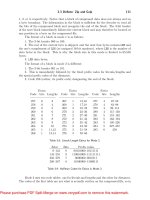
E x a m p l e 11 . 4 . 1 :
For the speech sequence shown in Figure 11.7, let us find predictors of orders one, two, and
three and examine their performance. We begin by estimating the autocorrelation values from
the data. Given M data points, we use the following average to find the value for Rx x (k):
Rx x (k) =

1
M −k

M−k

xi xi+k
i=1

3
2
1
0
−1
−2
−3
500
F I G U R E 11 . 7

1000 1500 2000 2500 3000 3500 4000

A segment of speech: a male speaker saying the word “test.”

(35)


11.4 Prediction in DPCM

355

3
2
1
0
−1
−2
−3
500
F I G U R E 11 . 8

1000 1500 2000 2500 3000 3500 4000

The residual sequence using a third- order predictor.

Using these autocorrelation values, we obtain the following coefficients for the three different predictors. For N = 1, the predictor coefficient is a1 = 0.66; for N = 2, the coefficients
are a1 = 0.596 and a2 = 0.096; and for N = 3, the coefficients are a1 = 0.577, a2 = −0.025,
and a3 = 0.204. We used these coefficients to generate the residual sequence. In order to see
the reduction in variance, we computed the ratio of the source output variance to the variance
of the residual sequence. For comparison, we also computed this ratio for the case where the
residual sequence is obtained by taking the difference of neighboring samples. The sample-tosample differences resulted in a ratio of 1.63. Compared to this, the ratio of the input variance

to the variance of the residuals from the first-order predictor was 2.04. With a second-order
predictor, this ratio rose to 3.37, and with a third-order predictor, the ratio was 6.28.
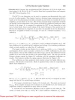
The residual sequence for the third-order predictor is shown in Figure 11.8. Notice that
although there has been a reduction in the dynamic range, there is still substantial structure
in the residual sequence, especially in the range of samples from about the 700th sample to
the 2000th sample. We will look at ways of removing this structure when we discuss speech
coding.
Let us now introduce a quantizer into the loop and look at the performance of the DPCM
system. For simplicity, we will use a uniform quantizer. If we look at the histogram of the
residual sequence, we find that it is highly peaked. Therefore, we will assume that the input
to the quantizer will be Laplacian. We will also adjust the step size of the quantizer based on
the variance of the residual. The step sizes provided in Chapter 9 are based on the assumption
that the quantizer input has a unit variance. It is easy to show that when the variance differs
from unity, the optimal step size can be obtained by multiplying the step size for a variance of
one with the standard deviation of the input. Using this approach for a four-level Laplacian
quantizer, we obtain step sizes of 0.75, 0.59, and 0.43 for the first-, second-, and third-order
predictors, and step sizes of 0.3, 0.4, and 0.5 for an eight-level Laplacian quantizer. We
measure the performance using two different measures, the signal-to-noise ratio (SNR) and


356

11

T A B L E 11 . 1

D I F F E R E N T I A L

Performance of DPCM system
with different predictors and

quantizers.

Quantizer

Predictor Order

SNR (dB)

Four-level

None
1
2
3
None
1
2
3

2.43
3.37
8.35
8.74
3.65
3.87
9.81
10.16

Eight-level

E N C O D I N G

SPER (dB)
0
2.65
5.9
6.1
0
2.74
6.37
6.71

the signal-to-prediction error ratio. These are defined as follows:
SNR(dB) = 10 log10
SPER(dB) = 10 log10

M
2
i=1 x i
M
2
i=1 (x i − xˆi )
M
2
i=1 x i
M
2
i=1 (x i − pi )

(36)

(37)

The results are tabulated in Table 11.1. For comparison we have also included the results
when no prediction is used; that is, we directly quantize the input. Notice the large difference
between using a first-order predictor and a second-order predictor, and then the relatively minor
increase when going from a second-order predictor to a third-order predictor. This is fairly
typical when using a fixed quantizer.
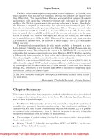
Finally, let’s take a look at the reconstructed speech signal. The speech coded using
a third-order predictor and an eight-level quantizer is shown in Figure 11.9. Although the
reconstructed sequence looks like the original, notice that there is significant distortion in
areas where the source output values are small. This is because in these regions the input to the
quantizer is close to zero. Because the quantizer does not have a zero output level, the output
of the quantizer flips between the two inner levels. If we listened to this signal, we would hear
a hissing sound in the reconstructed signal.
The speech signal used to generate this example is contained among the data sets accompanying this book in the file testm.raw. The function readau.c can be used to read the
file. You are encouraged to reproduce the results in this example and listen to the resulting
reconstructions.
If we look at the speech sequence in Figure 11.7, we can see that there are several distinct
segments of speech. Between sample number 700 and sample number 2000, the speech looks
periodic. Between sample number 2200 and sample number 3500, the speech is low amplitude
and noiselike. Given the distinctly different characteristics in these two regions, it would make
sense to use different approaches to encode these segments. Some approaches to dealing with


11.5 Adaptive DPCM

357

3
2

1
0
−1
−2
−3
500
F I G U R E 11 . 9

1000 1500 2000 2500 3000 3500 4000

The reconstructed sequence using a third- order predictor and an
eight- level uniform quantizer.

these issues are specific to speech coding, and we will encounter them when we specifically
discuss encoding speech using DPCM. However, the problem is also much more widespread
than when encoding speech. A general response to the nonstationarity of the input is the use
of adaptation in prediction. We will look at some of these approaches in the next section.

11.5

Adaptive DPCM

As DPCM consists of two main components, the quantizer and the predictor, making DPCM
adaptive means making the quantizer and the predictor adaptive. Recall that we can adapt a
system based on its input or output. The former approach is called forward adaptation; the
latter, backward adaptation. In the case of forward adaptation, the parameters of the system are
updated based on the input to the encoder, which is not available to the decoder. Therefore, the
updated parameters have to be sent to the decoder as side information. In the case of backward
adaptation, the adaptation is based on the output of the encoder. As this output is also available
to the decoder, there is no need for transmission of side information.

In cases where the predictor is adaptive, especially when it is backward adaptive, we
generally use adaptive quantizers (forward or backward). The reason for this is that the
backward adaptive predictor is adapted based on the quantized outputs. If for some reason
the predictor does not adapt properly at some point, this results in predictions that are far
from the input, and the residuals will be large. In a fixed quantizer, these large residuals will
tend to fall in the overload regions with consequently unbounded quantization errors. The
reconstructed values with these large errors will then be used to adapt the predictor, which will
result in the predictor moving further and further from the input.
The same constraint is not present for quantization, and we can have adaptive quantization
with fixed predictors.


358

11.5.1

11

D I F F E R E N T I A L

E N C O D I N G

Adaptive Quantization in DPCM

In forward adaptive quantization, the input is divided into blocks. The quantizer parameters are
estimated for each block. These parameters are transmitted to the receiver as side information.
In DPCM, the quantizer is in a feedback loop, which means that the input to the quantizer is not
conveniently available in a form that can be used for forward adaptive quantization. Therefore,
most DPCM systems use backward adaptive quantization.
The backward adaptive quantization used in DPCM systems is basically a variation of the

backward adaptive Jayant quantizer described in Chapter 9. In Chapter 9, the Jayant algorithm
was used to adapt the quantizer to a stationary input. In DPCM, the algorithm is used to adapt
the quantizer to the local behavior of nonstationary inputs. Consider the speech segment shown
in Figure 11.7 and the residual sequence shown in Figure 11.8. Obviously, the quantizer used
around the 3000th sample should not be the same quantizer that was used around the 1000th
sample. The Jayant algorithm provides an effective approach to adapting the quantizer to the
variations in the input characteristics.

E x a m p l e 11 . 5 . 1 :
Let’s encode the speech sample shown in Figure 11.7 using a DPCM system with a backward
adaptive quantizer. We will use a third-order predictor and an eight-level quantizer. We will
also use the following multipliers [124]:
M0 = 0.90 M1 = 0.90 M2 = 1.25 M3 = 1.75
The results are shown in Figure 11.10. Notice the region at the beginning of the speech
sample and between the 3000th and 3500th sample, where the DPCM system with the fixed
quantizer had problems. Because the step size of the adaptive quantizer can become quite
small, these regions have been nicely reproduced. However, right after this region, the speech
output has a larger spike than the reconstructed waveform. This is an indication that the
quantizer is not expanding rapidly enough. This can be remedied by increasing the value of
M3 . The program used to generate this example is dpcm_aqb. You can use this program to
study the behavior of the system for different configurations.

11.5.2

Adaptive Prediction in DPCM

The equations used to obtain the predictor coefficients were derived based on the assumption
of stationarity. However, we see from Figure 11.7 that this assumption is not true. In the
speech segment shown in Figure 11.7, different segments have different characteristics. This
is true for most sources we deal with; while the source output may be locally stationary over

any significant length of the output, the statistics may vary considerably. In this situation, it
is better to adapt the predictor to match the local statistics. This adaptation can be forward
adaptive or backward adaptive.


11.5 Adaptive DPCM

359

3
2
1
0
−1
−2
−3
500
F I G U R E 11 . 10

1000 1500 2000 2500 3000 3500 4000

The reconstructed sequence using a third- order predictor and an
eight- level Jayant quantizer.

DPCM with Forward Adaptive Prediction (DPCM-APF)

In forward adaptive prediction, the input is divided into segments or blocks. In speech coding
this block usually consists of about 16 ms of speech. At a sampling rate of 8000 samples per
second, this corresponds to 128 samples per block [134,172]. In image coding, we use an
8 × 8 block [173].

The autocorrelation coefficients are computed for each block. The predictor coefficients
are obtained from the autocorrelation coefficients and quantized using a relatively high-rate
quantizer. If the coefficient values are to be quantized directly, we need to use at least 12
bits per coefficient [134]. This number can be reduced considerably if we represent the
predictor coefficients in terms of parcor coefficients; we will describe how to obtain the parcor
coefficients in Chapter 17. For now, let’s assume that the coefficients can be transmitted with
an expenditure of about 6 bits per coefficient.
In order to estimate the autocorrelation for each block, we generally assume that the sample
values outside each block are zero. Therefore, for a block length of M, the autocorrelation
function for the lth block would be estimated by
Rx(l)x (k) =

1
M −k

l M−k

xi xi+k

(38)

i=(l−1)M+1

for k positive, or
Rx(l)x (k) =

1
M +k

lM

xi xi+k

(39)

i=(l−1)M+1−k

for k negative. Notice that Rx(l)x (k) = Rx(l)x (−k), which agrees with our initial assumption.


360

11

D I F F E R E N T I A L

E N C O D I N G

dn2

a1
F I G U R E 11 . 11

A plot of the residual squared versus the predictor coefficient.

DPCM with Backward Adaptive Prediction (DPCM-APB)

Forward adaptive prediction requires that we buffer the input. This introduces delay in the
transmission of the speech. As the amount of buffering is small, the use of forward adaptive
prediction when there is only one encoder and decoder is not a big problem. However, in

the case of speech, the connection between two parties may be several links, each of which
may consist of a DPCM encoder and decoder. In such tandem links, the amount of delay can
become large enough to be a nuisance. Furthermore, the need to transmit side information
makes the system more complex. In order to avoid these problems, we can adapt the predictor
based on the output of the encoder, which is also available to the decoder. The adaptation is
done in a sequential manner [172,174].
In our derivation of the optimum predictor coefficients, we took the derivative of the
statistical average of the squared prediction error or residual sequence. In order to do this, we
had to assume that the input process was stationary. Let us now remove that assumption and
try to figure out how to adapt the predictor to the input algebraically. To keep matters simple,
we will start with a first-order predictor and then generalize the result to higher orders.
For a first-order predictor, the value of the residual squared at time n would be given by
dn2 = (xn − a1 xˆn−1 )2

(40)

If we could plot the value of dn2 against a1 , we would get a graph similar to the one shown in
Figure 11.11. Let’s take a look at the derivative of dn2 as a function of whether the current value
of a1 is to the left or right of the optimal value of a1 —that is, the value of a1 for which dn2 is
minimum. When a1 is to the left of the optimal value, the derivative is negative. Furthermore,
the derivative will have a larger magnitude when a1 is further away from the optimal value. If
we were asked to adapt a1 , we would add to the current value of a1 . The amount to add would
be large if a1 was far from the optimal value, and small if a1 was close to the optimal value.
If the current value was to the right of the optimal value, the derivative would be positive, and
we would subtract some amount from a1 to adapt it. The amount to subtract would be larger if
we were further from the optimal, and as before, the derivative would have a larger magnitude
if a1 were further from the optimal value.


11.6 Delta Modulation

361

At any given time, in order to adapt the coefficient at time n + 1, we add an amount
proportional to the magnitude of the derivative with a sign that is opposite to that of the
derivative of dn2 at time n:
∂d 2
(n+1)
(n)
= a1 − α n
(41)
a1
∂a1
where α is some positive proportionality constant.
∂dn2
= −2(xn − a1 xˆn−1 )xˆn−1
∂a1
= −2dn xˆn−1 .

(42)
(43)

Substituting this into (41), we get
a1(n+1) = a1(n) + αdn xˆn−1

(44)

where we have absorbed the 2 into α. The residual value dn is available only to the encoder.
Therefore, in order for both the encoder and decoder to use the same algorithm, we replace dn
by dˆn in (44) to obtain

(n+1)
(n)
a1
= a1 + α dˆn xˆn−1
(45)
Extending this adaptation equation for a first-order predictor to an N th-order predictor is
relatively easy. The equation for the squared prediction error is given by
2

N

dn2

= xn −

ai xˆn−i

(46)

i=1

Taking the derivative with respect to a j will give us the adaptation equation for the jth predictor
coefficient:
(n+1)
(n)
= a j + α dˆn xˆn− j
(47)
aj
We can combine all N equations in vector form to get
A(n+1) = A(n) + α dˆn X n−1

where

⎡

xˆn

(48)

⎤

⎢ xˆn−1 ⎥
⎢
⎥
Xn = ⎢
⎥
...
⎣
⎦
xˆn−N +1

(49)

This particular adaptation algorithm is called the least mean squared (LMS) algorithm [175].

11.6

Delta Modulation

A very simple form of DPCM that has been widely used in a number of speech-coding applications is the delta modulator (DM). The DM can be viewed as a DPCM system with a 1-bit

362

F I G U R E 11 . 12

11

D I F F E R E N T I A L

E N C O D I N G

A signal sampled at two different rates.

(two-level) quantizer. With a two-level quantizer with output values ± , we can only represent
a sample-to-sample difference of . If, for a given source sequence, the sample-to-sample
difference is often very different from , then we may incur substantial distortion. One way
to limit the difference is to sample more often. In Figure 11.12 we see a signal that has been
sampled at two different rates. The lower-rate samples are shown by open circles, while the
higher-rate samples are represented by +. It is apparent that the lower-rate samples are not
only further apart in time, they are also further apart in value.
The rate at which a signal is sampled is governed by the highest frequency component of
a signal. If the highest frequency component in a signal is W , then in order to obtain an exact
reconstruction of the signal, we need to sample it at least at twice the highest frequency, or
2W (see Section 12.7). In systems that use delta modulation, we usually sample the signal at
much more than twice the highest frequency. If Fs is the sampling frequency, then the ratio of
Fs to 2W can range from almost 1 to almost 100 [134]. The higher sampling rates are used
for high-quality A/D converters, while the lower rates are more common for low-rate speech
coders.
If we look at a block diagram of a delta modulation system, we see that, while the block
diagram of the encoder is identical to that of the DPCM system, the standard DPCM decoder is

followed by a filter. The reason for the existence of the filter is evident from Figure 11.13, where
we show a source output and the unfiltered reconstruction. The samples of the source output
are represented by the filled circles. As the source is sampled at several times the highest
frequency, the staircase shape of the reconstructed signal results in distortion in frequency
bands outside the band of frequencies occupied by the signal. The filter can be used to remove
these spurious frequencies.
The reconstruction shown in Figure 11.13 was obtained with a delta modulator using a
fixed quantizer. Delta modulation systems that use a fixed step size are often referred to as
linear delta modulators. Notice that the reconstructed signal shows one of two behaviors. In
regions where the source output is relatively constant, the output alternates up or down by ;
these regions are called the granular regions. In the regions where the source output rises or
falls fast, the reconstructed output cannot keep up; these regions are called the slope overload
regions. If we want to reduce the granular error, we need to make the step size
small.
However, this will make it more difficult for the reconstruction to follow rapid changes in the
input. In other words, it will result in an increase in the overload error. To avoid the overload
condition, we need to make the step size large so that the reconstruction can quickly catch up
with rapid changes in the input. However, this will increase the granular error.


11.6 Delta Modulation

363

Slope overload
region

Granular region

F I G U R E 11 . 13

A source output sampled and coded using delta modulation.

Slope overload
region

Granular region

F I G U R E 11 . 14

A source output sampled and coded using adaptive delta modulation.

One way to avoid this impasse is to adapt the step size to the characteristics of the input, as
shown in Figure 11.14. In quasi-constant regions, make the step size small in order to reduce
the granular error. In regions of rapid change, increase the step size in order to reduce overload
error. There are various ways of adapting the delta modulator to the local characteristics of
the source output. We describe two of the more popular ways here.

11.6.1

Constant Factor Adaptive Delta Modulation
(CFDM)

The objective of adaptive delta modulation is clear: increase the step size in overload regions
and decrease it in granular regions. The problem lies in knowing when the system is in each
of these regions. Looking at Figure 11.13, we see that in the granular region the output of the
quantizer changes sign with almost every input sample; in the overload region, the sign of the
quantizer output is the same for a string of input samples. Therefore, we can define an overload
or granular condition based on whether the output of the quantizer has been changing signs.
A very simple system [176] uses a history of one sample to decide whether the system is in

overload or granular condition and whether to expand or contract the step size. If sn denotes


364

11

D I F F E R E N T I A L

E N C O D I N G

the sign of the quantizer output dˆn ,
sn =

1 if
−1 i f

dˆn > 0
dˆn < 0

(50)

= sn−1
sn = sn−1

(51)

the adaptation logic is given by
n

=

M1
M2

n−1 sn
n−1

where M1 = M12 = M > 1. In general, M < 2.
By increasing the memory, we can improve the response of the CFDM system. For example,
if we looked at two past samples, we could decide that the system was moving from overload
to granular condition if the sign had been the same for the past two samples and then changed
with the current sample:
(52)
sn = sn−1 = sn−2
In this case it would be reasonable to assume that the step size had been expanding previously
and, therefore, needed a sharp contraction. If
sn = sn−1 = sn−2

(53)

then it would mean that the system was probably entering the overload region, while
sn = sn−1 = sn−2

(54)

would mean the system was in overload and the step size should be expanded rapidly.
For the encoding of speech, the following multipliers Mi are recommended by [177] for a
CFDM system with two-sample memory:
sn = sn−1 sn−2

M1 = 0.4

(55)

sn = sn−1 = sn−2
sn = sn−1 = sn−2
sn = sn−1 = sn−2

M2 = 0.9
M3 = 1.5
M4 = 2.0

(56)
(57)
(58)

The amount of memory can be increased further with a concurrent increase in complexity. The
space shuttle used a delta modulator with a memory of seven [178].
11.6.2

Continuously Variable Slope Delta Modulation

The CFDM systems described use a rapid adaptation scheme. For low-rate speech coding, it is
more pleasing if the adaptation is over a longer period of time. This slower adaptation results in
a decrease in the granular error and generally an increase in overload error. Delta modulation
systems that adapt over longer periods of time are referred to as syllabically companded. A
popular class of syllabically companded delta modulation systems are continuously variable
slope delta modulation systems.

11.7 Speech Coding

365

1.0
0.8
0.6
0.4
0.2
0
−0.2
−0.4
0
F I G U R E 11 . 15

20

40

60

80

100

Autocorrelation function for test.snd.

The adaptation logic used in CVSD systems is as follows [134]:
n

=β

n−1

+ αn

0

(59)

where β is a number less than but close to one, and αn is equal to one if J of the last K
quantizer outputs were of the same sign. That is, we look in a window of length K to obtain
the behavior of the source output. If this condition is not satisfied, then αn is equal to zero.
Standard values for J and K are J = 3 and K = 3.

11.7

Speech Coding

Differential encoding schemes are immensely popular for speech encoding. They are used in
the telephone system, voice messaging, and multimedia applications, among others. Adaptive
DPCM is a part of several international standards (ITU-T G.721, ITU G.723, ITU G.726,
ITU-T G.722), which we will look at here and in later chapters.
Before we do that, let’s take a look at one issue specific to speech coding. In Figure 11.7,
we see that there is a segment of speech that looks highly periodic. We can see this periodicity
if we plot the autocorrelation function of the speech segment (Figure 11.15).
The autocorrelation peaks at a lag value of 47 and multiples of 47. This indicates a
periodicity of 47 samples. This period is called the pitch period. The predictor we originally
designed did not take advantage of this periodicity, as the largest predictor was a third-order

predictor, and this periodic structure takes 47 samples to show up. We can take advantage of
this periodicity by constructing an outer prediction loop around the basic DPCM structure as
shown in Figure 11.16. This can be a simple single coefficient predictor of the form b xˆn−τ ,
where τ is the pitch period. Using this system on testm.raw, we get the residual sequence
shown in Figure 11.17. Notice the decrease in amplitude in the periodic portion of the speech.
Finally, remember that we have been using mean squared error as the distortion measure in
all of our discussions. However, perceptual tests do not always correlate with the mean squared


366

11

xn
+

–

^

dn

+
–
pn

^

dn

Q
pn

D I F F E R E N T I A L

dn +

+

+

pn

E N C O D I N G

xn

+
+

+
P

PP

Decoder
P

+

Encoder

+
x^ n

Pp
F I G U R E 11 . 16

The DPCM structure with a pitch predictor.

3
2
1
0
−1
−2
−3
500
F I G U R E 11 . 17

1000 1500 2000 2500 3000 3500 4000

The residual sequence using the DPCM system with a pitch
predictor.

error. The level of distortion we perceive is often related to the level of the speech signal. In
regions where the speech signal is of higher amplitude, we have a harder time perceiving the
distortion, but the same amount of distortion in a different frequency band, where the speech
is of lower amplitude, might be very perceptible. We can take advantage of this by shaping
the quantization error so that most of the error lies in the region where the signal has a higher

amplitude. This variation of DPCM is called noise feedback coding (NFC) (see [134] for
details).

11.7.1

G.726

The International Telecommunications Union has published several recommendations for a
standard ADPCM system, including recommendations G.721, G.723, and G.726. G.726 supersedes G.721 and G.723. In this section we will describe the G.726 recommendation for
ADPCM systems at rates of 40, 32, 24, and 16 kbits.


11.7 Speech Coding

367

T A B L E 11 . 2

Recommended input- output
characteristics of the quantizer
for 24- kbits- per- second
operation.

Input Range

Label

Output

log2 αdkk

|Ik |
3
2
1
0

log2 αdkk
2.91
2.13
1.05
−∞

[2.58, ∞)
[1.70, 2.58)
[0.06, 1.70)
(−∞, −0.06)

The Quantizer

The recommendation assumes that the speech output is sampled at the rate of 8000 samples
per second, so the rates of 40, 32, 24, and 16 kbits per second translate 5 bits per sample, 4
bits per sample, 3 bits per sample, and 2 bits per sample. Comparing this to the PCM rate of
8 bits per sample, this would mean compression ratios of 1.6:1, 2:1, 2.67:1, and 4:1. Except
for the 16 kbits per second system, the number of levels in the quantizer are 2n b − 1, where
n b is the number of bits per sample. Thus, the number of levels in the quantizer is odd, which
means that for the higher rates we use a midtread quantizer.
The quantizer is a backward adaptive quantizer with an adaptation algorithm that is similar
to the Jayant quantizer. The recommendation describes the adaptation of the quantization
interval in terms of the adaptation of a scale factor. The input dk is normalized by a scale

factor αk . This normalized value is quantized, and the normalization removed by multiplying
with αk . In this way the quantizer is kept fixed and αk is adapted to the input. Therefore, for
example, instead of expanding the step size, we would increase the value of αk .
The fixed quantizer is a nonuniform midtread quantizer. The recommendation describes
the quantization boundaries and reconstruction values in terms of the log of the scaled input.
The input-output characteristics for the 24 kbit system are shown in Table 11.2. An output
value of −∞ in the table corresponds to a reconstruction value of 0.
The adaptation algorithm is described in terms of the logarithm of the scale factor:
y(k) = log2 αk

(60)

The adaptation of the scale factor α or its log y(k) depends on whether the input is speech or
speechlike, where the sample-to-sample difference can fluctuate considerably, or whether the
input is voice-band data, which might be generated by a modem, where the sample-to-sample
fluctuation is quite small. In order to handle both these situations, the scale factor is composed
of two values, a locked slow scale factor for when the sample-to-sample differences are quite
small, and an unlocked value for when the input is more dynamic:
y(k) = al (k)yu (k − 1) + (1 − al (k))yl (k − 1)

(61)

The value of al (k) depends on the variance of the input. It will be close to one for speech
inputs and close to zero for tones and voice-band data.


368

11

D I F F E R E N T I A L

E N C O D I N G

The unlocked scale factor is adapted using the Jayant algorithm with one slight modification. If we were to use the Jayant algorithm, the unlocked scale factor could be adapted as
αu (k) = αk−1 M[Ik−1 ]

(62)

where M[·] is the multiplier. In terms of logarithms, this becomes
yu (k) = y(k − 1) + log M[Ik−1 ]

(63)

The modification consists of introducing some memory into the adaptive process so that the
encoder and decoder converge following transmission errors:
yu (k) = (1 − )y(k − 1) + W [Ik−1 ]

(64)

where W [·] = log M[·], and = 2−5 .
The locked scale factor is obtained from the unlocked scale factor through
γ = 2−6

yl (k) = (1 − γ )yl (k − 1) + γ yu (k),

(65)

The Predictor

The recommended predictor is a backward adaptive predictor that uses a linear combination
of the past two reconstructed values as well as the six past quantized differences to generate
the prediction:
2

(k−1)

pk =

ai

6

xˆk−i +

i=1

(k−1)

bi

dˆk−i

(66)

i=1

The set of predictor coefficients is updated using a simplified form of the LMS algorithm:
(k)

(k−1)

a1 = (1 − 2−8 )a1
(k)
a2

=

+ 3 × 2−8 sgn[z(k)]sgn[z(k − 1)]

(k−1)
(1 − 2 )a2
+ 2−7 (sgn[z(k)]sgn[z(k
(k−1)
sgn[z(k)]sgn[z(k − 1)] )
− f a1
−7

where
z(k) = dˆk +

6

(k−1)

bi

(67)

− 2)]

dˆk−i

(68)

(69)

i=1

f (β) =

|β|
4β
2sgn(β) |β| >

1
2
1
2

(70)

The coefficients {bi } are updated using the following equation:
bi(k) = (1 − 2−8 )bi(k−1) + 2−7 sgn[dˆk ]sgn[dˆk−i ]

(71)

Notice that in the adaptive algorithms we have replaced products of reconstructed values
and products of quantizer outputs with products of their signs. This is computationally much
simpler and does not lead to any significant degradation of the adaptation process. Furthermore,

the values of the coefficients are selected such that multiplication with these coefficients can


11.8 Image Coding

369

be accomplished using shifts and adds. The predictor coefficients are all set to zero when the
input moves from tones to speech.

11.8

Image Coding

We saw in Chapter 7 that differential encoding provided an efficient approach to the lossless
compression of images. The case for using differential encoding in the lossy compression of
images has not been made as clearly. In the early days of image compression, both differential
encoding and transform coding were popular forms of lossy image compression. At the
current time differential encoding has a much more restricted role as part of other compression
strategies. Several currently popular approaches to image compression decompose the image
into lower and higher frequency components. As low-frequency signals have high sample-tosample correlation, several schemes use differential encoding to compress the low-frequency
components. We will see this use of differential encoding when we look at subband- and
wavelet-based compression schemes and, to a lesser extent, when we study transform coding.
For now let us look at the performance of a couple of stand-alone differential image compression schemes. We will compare the performance of these schemes with the performance
of the JPEG compression standard.
Consider a simple differential encoding scheme in which the predictor p[ j, k] for the pixel
in the jth row and the kth column is given by
⎧
ˆ j, k − 1] for k > 0
⎨ x[

ˆ j − 1, k] for k = 0 and j > 0
p[ j, k] = x[
⎩
128
for j = 0 and k = 0
where x[
ˆ j, k] is the reconstructed pixel in the jth row and kth column. We use this predictor in
conjunction with a fixed four-level uniform quantizer and code the quantizer output using an
arithmetic coder. The coding rate for the compressed image is approximately 1 bit per pixel.
We compare this reconstructed image with a JPEG-coded image at the same rate in Figure
11.18. The signal-to-noise ratio for the differentially encoded image is 22.33 dB (PSNR 31.42
dB), while for the JPEG-encoded image it is 32.52 dB (PSNR 41.60 dB), a difference of more
than 10 dB!
However, this is an extremely simple system compared to the JPEG standard, which has
been fine-tuned for encoding images. Let’s make our differential encoding system slightly
more complicated by replacing the uniform quantizer with a recursively indexed quantizer and
by using a somewhat more complex predictor. For each pixel (except for the boundary pixels)
we compute the following three values:
ˆ j − 1, k] + 0.5 × x[
ˆ j, k − 1]
p1 = 0.5 × x[
ˆ j − 1, k − 1] + 0.5 × x[
ˆ j, k − 1]
p2 = 0.5 × x[
ˆ j − 1, k − 1] + 0.5 × x[
ˆ j − 1, k]
p3 = 0.5 × x[
then obtain the predicted value as
p[ j, k] = median{ p1 , p2 , p3 }

(72)