The Temporal Pattern of Mortality Responses to Air Pollution: A Multicity Assessment of Mortality Displacement potx

The Temporal Pattern of Mortality Responses
to Air Pollution:
A Multicity Assessment of Mortality Displacement
Antonella Zanobetti,
1
Joel Schwartz,
1
Evi Samoli,
2
Alexandros Gryparis,
2
Giota Touloumi,
2
Richard Atkinson,
3
Alain Le Tertre,
4
Janos Bobros,
5
Martin Celko,
6
Ayana Goren,
7
Bertil Forsberg,
8
Paola Michelozzi,
9
Daniel Rabczenko,
10
Emiliano Aranguez Ruiz,
11

and Klea Katsouyanni
2
Abstract: Although the association between particulate matter
and mortality or morbidity is generally accepted, controversy
remains about the importance of the association. If it is due solely
to the deaths of frail individuals, which are brought forward by
only a brief period of time, the public health implications of the
association are fewer than if there is an increase in the number of
deaths. Recently, other research has addressed the mortality dis-
placement issue in single-city analysis. We analyzed this issue with
a distributed lag model in a multicity hierarchic modeling ap-
proach, within the Air Pollution and Health: A European Ap-
proach (APHEA-2) study. We fit a Poisson regression model and
a polynomial distributed lag model with up to 40 days of delay in
each city. In the second stage we combined the city-specific
results. We found that the overall effect of particulate matter less
than 10
␮
M in aerodynamic diameter (PM
10
) per 10
␮
g/m
3
for
the fourth-degree distributed lag model is a 1.61% increase in
daily deaths (95% CI ϭ 1.02–2.20), whereas the mean of PM
10
on
the same day and the previous day is associated with only a 0.70%

increase in deaths (95% CI ϭ 0.43– 0.97). This result is un-
changed using an unconstrained distributed lag model. Our study
confirms that the effects observed in daily time-series studies are
not due primarily to short-term mortality displacement. The effect
size estimate for airborne particles more than doubles when we
consider longer-term effects, which has important implications for
risk assessment. (E
PIDEMIOLOGY 2002;13:87–93)
Key words: air pollution, mortality, mortality displacement.
A
ir pollution, especially airborne particles, has
been consistently reported to be associated with
daily deaths in reports from all over the
world.
1– 8
More recently, systematic multicity analyses
have confirmed these findings.
9 –12
Nevertheless, some
have questioned the public health significance of these
associations, arguing that if these deaths are occurring
only in those who would have died in a few days anyway,
the public health significance of exposure is small. Were
that the case, the increase in deaths during and imme-
diately after exposure would be counterbalanced by a
deficit in daily deaths a few days later, when those deaths
would have otherwise occurred. If such a pattern were
true, the positive correlation seen between daily deaths
and exposure shortly before the death would be coun-
terbalanced by a negative correlation between exposure

and daily deaths at some longer lag. An example of such
a hypothetical pattern, called mortality displacement or
harvesting effect, is seen in Figure 1. Were such a phe-
nomenon to exist, it should be detected readily in studies
of acute episodes, but those patterns have not been
observed in air pollution episodes.
13
It is useful to examine the reason for such a phenom-
enon. Assume there is a pool of people at high risk of
dying at any given time. An air pollution episode, by
From the
1
Environmental Epidemiology Program, Harvard School of Public
Health, Boston, MA;
2
University of Athens Medical School, Athens, Greece;
3
Department of Public Health Sciences, St George’s Hospital Medical School,
London, United Kingdom;
4
Environmental Health Unit, National Institute of
Public Health Surveillance, Saint-Maurice, France;
5
Municipal Institute of Pub-
lic Health, Budapest, Hungary;
6
Charles University Medical Faculty, Prague,
Czech Republic;
7
Department of Epidemiology, Tel Aviv University, Tel Aviv,

Israel;
8
Department of Public Health and Clinical Medicine, Umeå University,
Umeå, Sweden;
9
Agency for Public Health, Lazio Region, Rome, Italy;
10
Na-
tional Institute of Hygiene, Department of Medical, Statistics, Warsaw, Poland;
and
11
Municipal Department of Public Health, Madrid, Spain.
Address correspondence to: Antonella Zanobetti, Department of Environmental
Health, Environmental Epidemiology Program, Harvard School of Public Health,
665 Huntington Avenue, Boston, MA 02115; azanob@sparc6a. harvard.edu
This research was part of the APHEA-2 project, which was funded by the
European Union contract number ENV4-CT97-0534. Joel Schwartz was also
supported by U.S. Environmental Protection Agency Grant R827353.
Submitted October 16, 2000; final version accepted August 21, 2001.
Copyright © 2001 by Lippincott Williams & Wilkins, Inc.
87
increasing the risk in that pool, would increase the death
rate out of the pool and result in a smaller pool size. The
finite size of the risk pool creates the possibility of a
negative association with pollution at some lags. This
rebound (ie, drop in the number of deaths, after an
initial increase) presupposes that air pollution does not
affect recruitment into the pool. Yet numerous epidemi-
ologic studies have shown particulate air pollution to be
associated with exacerbation of illness, including in-

creased hospitalizations,
14
decreased heart rate variabil-
ity,
15
etc, thus suggesting that increased recruitment is
possible. Recently, Zelikoff et al
16
have shown that par-
ticle exposure exacerbates pneumonia in animals.
Hence, air pollution may intensify some illnesses, in-
creasing the size of the risk pool. Further, this may occur
with a different lag than that between exposure and
death out of the risk pool. Hence, the direction of the
effect of an air pollution episode on the size of the risk
pool, and the effect of the risk pool on the death rate
over time, may be positive or negative.
Recently, three papers have examined this issue in-
directly, by estimating the association between air pol-
lution and daily deaths in Philadelphia,
17
Boston,
18
and
Chicago
19
after filtering out such rebounds. None of the
studies found any evidence that the effect size for air
pollution was reduced as a result of the mortality dis-
placement, and indeed all three studies reported that the

effect size approximately doubled. Schwartz
18
interpreted
this as suggesting that, far from depleting the pool of
critically ill people, air pollution increased the size of the
pool over longer time scales by increasing the intensity
of illness in general. None of these studies provided any
direct estimate of what the time course of the rise and
fall of mortality after exposure might be (eg, Figure 1).
One additional analysis has recently been pub-
lished.
20
These authors assumed a model in which air
pollution could only deplete the pool of susceptible
individuals at high risk of dying and could not increase
recruitment into that pool. This is equivalent to assum-
ing that the correlation between air pollution and daily
deaths must become negative after a lag of several days.
That assumption is a testable hypothesis.
Another recent paper
21
applied a different approach
that explicitly tests this hypothesis. Zanobetti et al
21
estimated the association of air pollution at multiple lags
simultaneously, providing a direct estimate of Figure 1.
Because air pollution is generally correlated, putting a
large number of lags of a pollutant into a model produces
high levels of multicolinearity and unstable results. To
counter this problem, these authors used a nonparamet-

ric smoothed distributed lag, looking out to 40 days after
exposure, to estimate the effect of air pollution on daily
deaths in Milan between 1980 and 1989. This con-
strained the estimated effects of air pollution to vary
smoothly with the number of days of lag between expo-
sure and death. This required special software that is not
generally available. However, in a sensitivity analysis,
they showed that essentially identical results could be
obtained using a cubic polynomial distributed lag model,
which can be implemented in any Poisson regression
package. In both cases, the coefficients of air pollution at
each lag are constrained to fit a smooth shape, in which
the latter case is a polynomial. If the polynomial is
flexible enough to fit the true pattern of the data rea-
sonably well, little bias will be introduced.
We have adopted that approach for a systematic
examination of the lag between air pollution and daily
deaths in the Air Pollution and Health: A European
Approach (APHEA-2) study.
22,23
This analysis focuses
on particulate air pollution in a multicity hierarchic
model.
Subjects and Methods
Health Data
The APHEA-2 study is a comprehensive, multicenter
study that examines the association between air pollu-
tion and daily deaths in 30 cities across Europe and
associated regions (eg, Tel Aviv). Data collection in-
cluded daily counts of all-cause mortality, excluding

deaths from external causes (International Classification of
Diseases, 9th revision, code Ͼ800). The years of study
were 1990 through 1997, although mortality data in
most cities were available only through 1995 or 1996. In
some cases, air pollution data were available only for part
of the period.
Because of resource and time constraints, it was de-
cided a priori to limit the analysis of mortality displace-
ment to ten cities. To maximize the power of the study,
we chose the largest cities in the study, with the stipu-
lation that only one city could be chosen in each coun-
try. The ten cities selected were Athens, Budapest, Lodz,
London, Madrid, Paris, Prague, Rome, Stockholm, and
FIGURE 1. Hypothetical lag structure corresponding to the
mortality displacement effect.
88 Zanobetti et al EPIDEMIOLOGY January 2002, Vol. 13 No. 1
Tel Aviv. Together, they comprise a population of about
28 million people, which is two-thirds of the population
in the full study, and they represent northern Europe,
central Europe, and the Mediterranean region. An ear-
lier paper
23
examined the association of particulate air
pollution in all available cities and addressed the issue of
heterogeneity in response. That analysis did not exam-
ine the “harvesting” issue addressed in this paper.
Daily measurements of particulate air pollution were
provided by each city participating in the APHEA-2
project. Particulate matter was measured as PM
10

(par-
ticulate air matter less than 10
␮
M in aerodynamic
diameter) in four cities, as PM
13
(particulate air matter
with aerodynamic diameter less than 13
␮
M) in Paris,
and PM
15
(particulate air matter with aerodynamic di-
ameter less than 15
␮
M) in Rome. The Paris data were
assumed to be equivalent to PM
10
in this study. Rome
data were converted to PM
10
using a site-specific con-
version factor based on colocated measurements.
24
In
Athens, data were routinely collected only on black
smoke. Because traffic is the dominant source of particles
in Athens, there were some days of colocated PM
10
and

black smoke monitoring that allowed the establishment
of a site-specific selective conversion. Also in Lodz only
data for black smoke were available, whereas in Budapest
the original data were measured as total suspended par-
ticulate. In these three cities, data were converted to
PM
10
as a function of both black smoke (total suspended
particulate for Budapest) and season, again on the basis
of regression modeling with limited PM
10
data.
We conducted a weighted metaregression with a
dummy variable equal to 1 for cities where the other
particle measures were converted to PM
10
on the basis of
site-specific calibration. We found a somewhat higher
coefficient in the converted cities (1.98% per 10
␮
g/m
3
increase in PM
10
compared with 1.48% in the cities that
measured PM
10
), but the confidence interval for the
incremental 0.5% effect was Ϯ1.93%. These results in-
dicate that the coefficients could in fact be 0. Further,

three of the five cities where the conversion occurred
were in southern Europe, where a previous hierarchic
model of all 29 cities in APHEA-2 showed larger coef-
ficients. We conclude that there is little reason to be-
lieve the effect estimates differ between the cities where
the air pollutant measurement has been converted and
the other cities. Hence, results were reported as the
effect of PM
10
. Further details have been previously
reported.
23
Covariate Control
Generalized additive regression models
25
were fitted
in each of the ten cities, controlling for seasonal pat-
terns, long-term time trends for weather, influenza epi-
demics, holidays, and day of the week. The models were
built following the APHEA-2 methodology.
23
Because of
the substantial variability in seasonal patterns and
weather between, for example, Stockholm and Tel Aviv,
separate models were chosen in each city. All models
controlled for temperature and humidity on the same
day using nonparametric smooth function.
27
In addition,
we examined whether nonparametric functions of

weather variables on the previous day or up to 3 previous
days or the average of a few days improved model fit
(defined as lowering the Akaike information criterion
28
for the model). We similarly chose the number of de-
grees of freedom for each weather variable to minimize
the Akaike information criterion. This approach has
been used and discussed previously.
29,30
Seasonal patterns are controlled because there are
unmeasured predictors of death, such as diet, which vary
seasonally and have long-term trends over time. Because
air pollution also shows seasonal variations and long-
term trends, this creates a potential for confounding.
Shorter-term fluctuations in diet are unlikely to be cor-
related with air pollution. Hence, the goal of our smooth
function of time is to remove seasonal and long-term
fluctuations.
Various smoothing parameters exist for producing
residuals with no seasonality. To choose among them,
we examined the partial autocorrelation function of the
residuals. This is because, although each death is an
independent event, seasonal patterns in the mortality
data produce correlations between the number of deaths
on one day and on the previous day. Eliminating short-
term serial correlation is therefore a measure of how
successful our seasonal control has been. On the other
hand, the use of excessive degrees of freedom for sea-
sonal control induces negative serial correlation in the
residuals of the mortality series,

31
which can distort the
association with air pollution. Therefore, we chose a
smoothing parameter for time to reduce the residuals to
white noise. Sometimes it was necessary to introduce
autoregressive terms to accomplish this.
32
This approach
has been used in a number of recent studies.
6,12,30
Distributed Lag Model
The goal of our analysis was to estimate the depen-
dence of daily deaths (on day t)onPM
10
on that day and
up to the previous 40 days. If the pollution-related
deaths are only being advanced by a few days to a few
weeks, we will see this effect as a negative association
between air pollution and deaths several days to several
weeks subsequently. The net effect of air pollution, net
of any such short-term rebound up to 40 days, is the sum
of the effect estimates for all 41 days. In addition, plot-
ting individual effect size estimates vs lag number gives
us a direct estimate of what Figure 1 really looks like.
This is an example of a distributed lag model, which has
been described previously.
33,34
EPIDEMIOLOGY January 2002, Vol. 13 No. 1 AIR POLLUTION AND MORTALITY DISPLACEMENT 89
For Poisson regression, the unconstrained distributed
lag model may be written as:

Log(E[Y
t
]) ϭ
␣
ϩ covariates ϩ
␤
0
Z
t
ϩ
␤
1
Z
tϪ1
ϩ
ϩ
␤
q
Z
tϪq
(1)
where Z
t
ϭ pollution variable delayed over time, for
j ϭ 0 q days.
Because this model produces unstable estimates for
large q, it is common to constrain the coefficients to vary
smoothly with lag number.
33
A polynomial distributed

lag constrains the
␤
j
to follow a polynomial pattern in
the lag number, that is:
␤
j
ϭ
͸
kϭ0
d
␩
k
j
k
, for j ϭ 0 q (2)
where j is the number of lag of delay and k is the
degree of the polynomial. Further details, including how
to estimate the
␩
k
in a Poisson model, have been pub-
lished previously.
34
Too much constraint risks bias, pro-
ducing a distorted shape, whereas too little constraint
produces estimates that are too noisy to be informative.
Although a cubic polynomial was sufficient to match the
results of the smoothed distributed lag in Milan,
21

we
have chosen a fourth-degree polynomial in this study, to
ensure enough degrees of freedom to fit the pattern of
response over time. Such a polynomial has enough de-
grees of freedom to model a curve such as that shown in
Figure 1, or any other plausible shape. Therefore, we
estimated in each city the five coefficients
␩
0

␩
4
for
the fourth-degree polynomial that defines the shape of
the distributed lag. As a sensitivity analysis, we used a
cubic polynomial and an unconstrained distributed lag
model. The unconstrained distributed lag model is too
noisy to provide any information about the shape of the
effect size vs lag, but it does give an unbiased estimate of
the overall effect. A separate distributed lag model was
fit for each of the ten cities.
Second-Stage Modeling
The hierarchic model has two stages. In the first
stage, the
ˆ
␩
ik
values are estimated in each city i,as
described in Eqs 1 and 2.
In the second stage, we combined the city-specific

coefficients
␩
ik
, using the multivariate maximum likeli-
hood method.
35
We assume that:
␩
ˆ
i
ϳ MVN͑
␩
k
,S
ˆ
i
ϩ D)
where
ˆ
␩
i
is the vector of
␩
k
in city i,
ˆ
S
i
is the estimated
variance-covariance matrix in city i, and D is the ran-

dom variance-covariance matrix component, reflecting
heterogeneity in response among the cities.
After combining the coefficients
ˆ
␩
ik
by city, the com-
bined coefficients by lag (
ˆ
␤
j
) for the distributed lag
model were obtained from Eq 2.
To see how the results compare with more traditional
models, we fit the same model in each city using as our
exposure index the mean PM
10
concentration on the day
of death and the previous day.
11,34,36,37
Note that this
model is a highly constrained variant of our distributed
lag model, with the constraints forcing
␤
1
ϭ
␤
0
, and
␤

2
ϭ
␤
3
ϭ ϭ
␤
40
ϭ 0. All analyses were done using the
S-plus software (Mathsoft Inc, Seattle, WA).
Results
Table 1 shows the ten cities, their populations, the
study period in each location, and the mean and stan-
dard deviation of the number of daily deaths and envi-
ronmental variables. Further details of the baseline mod-
els for each city have been published previously.
23
Table 2 shows, for each city, the estimated regression
coefficients of PM
10
(per 10
␮
g/m
3
and its 95% confi-
dence interval) for the traditional model (mean of the
current and previous day), and the overall effect from
the fourth-degree polynomial, the cubic, and unre-
TABLE 1. Study Period, Population, Mean, and Standard Deviation of the Number of Daily Deaths and the Environmental
Variables in the Ten Cities
Years of

Study
Population
(ϫ1,000)
Total Mortality PM
10
(
␮
g/m
3
)
5th–95th
Percentile
Temperature Humidity
Mean SD Mean SD Mean SD Mean SD
Athens 1992–1996 3073 72.9 13.2 42.7 12.9 33.4 –48.7 17.8 7.4 61.7 13.6
Budapest 1992–1995 1931 80.0 11.6 41.0 9.1 34.2 –45.6 12.8 8.8 70.1 12.6
Lodz 1990–1996 828 29.5 6.3 53.5 15.5 40.7 –61.9 8.4 8.4 79.0 12.4
London 1992–1996 6905 168.5 25.2 28.8 13.7 19.3 –34.0 11.8 5.4 69.3 11.3
Madrid 1992–1995 3012 60.8 11.1 37.8 17.7 26.9 –41.7 14.5 7.4 61.8 16.7
Paris 1992–1996 6700 123.3 15.7 22.5 11.5 14.5 –27.9 12.1 6.5 75.6 12.5
Prague 1992–1995 1212 38.2 7.2 76.2 45.7 46.9 –91.4 11.0 8.0 69.4 14.1
Rome 1992–1996 2775 56.2 10.4 58.7 17.4 61.8 –92.2 16.8 6.7 61.6 11.9
Stockholm 1994–1996 1126 28.9 6.1 15.5 7.9 9.9 –19.5 7.7 8.1 71.4 15.8
Tel Aviv 1993–1996 1141 27.4 6.3 50.3 57.5 32.0 –55.0 20.6 5.4 65.6 11.0
90 Zanobetti et al EPIDEMIOLOGY January 2002, Vol. 13 No. 1
stricted distributed lag models. The overall effect is the
sum of the
␤
j
per 10

␮
g/m
3
. It also shows the combined
effect estimates across all of the ten cities, based on a
random-effect model to combine results across cities.
Apart from Rome, the estimated effect of PM
10
in-
creased, and in many cities was more than doubled,
when the lagged effects were considered, rather than
reduced. These results are seen in all of the distributed
lag models that we applied, including the unconstrained
model.
The reason for this increase is clear from Figure 2,
which shows the estimated effect at each lag, and its
confidence interval from the fourth-degree polynomial.
It shows that the effect of PM
10
does decrease to close to
0 with a lag of 10 days, but remains positive, and rises
again to a second smaller peak, before dying out to 0 by
lag 40.
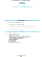
Figure 3 shows the combined effect for the cubic
polynomial. The PM
10
effect decreases with a minimum
at 14 days of lag and then rises again. Although they
differ in some detail, both figures show the same general
pattern. The initial effect declines to 0 with a lag of 1–2

weeks and then shows a second peak.
To test whether the effect at longer lags made an
important contribution to the overall effect, we com-
puted the overall effect (and its standard error) for the
first 10 days and for days 11– 40 before the death. The
effect estimate (ϫ1000) was 0.922 Ϯ 0.184 for the first
10 days of exposure, and 0.688 Ϯ 0.261 for the deaths
associated with PM
10
11– 40 days before. Hence, al-
though the exposure in the first week (and indeed the
first 2 days) before the event had a stronger impact, the
exposure in the preceding month substantially increased
the estimate of the overall effect.
TABLE 2. Results for the Ten Cities and Combined for the Estimated Particulate Matter <10
␮
M in Diameter (PM
10
)
Effect (؋1,000) for the Mean of PM
10
Lags 0–1, and the Cubic, Fourth-Degree, and Unrestricted Distributed Lag Models for
40 Lags
Mean 0–1* Cubic† 4th degree‡ Unrestricted§
bSEt bSEt bSEt bSEt
Athens 1.64 0.29 5.60 3.26 0.57 5.67 3.54 0.57 6.16 3.49 0.57 6.10
Budapest 0.28 0.46 0.61 1.20 0.85 1.41 1.41 0.86 1.65 1.01 0.87 1.16
Lodz 0.59 0.42 1.41 3.99 0.61 6.57 3.88 0.62 6.30 3.44 0.62 5.51
London 0.70 0.18 3.94 1.05 0.44 2.38 1.17 0.44 2.63 1.15 0.44 2.59
Madrid 0.52 0.24 2.22 2.35 0.52 4.53 2.34 0.52 4.52 2.57 0.52 4.92

Paris 0.42 0.23 1.82 2.48 0.46 5.40 2.54 0.46 5.53 2.45 0.46 5.30
Prague 0.11 0.18 0.60 0.66 0.33 1.99 0.72 0.34 2.13 0.53 0.35 1.49
Rome 1.51 0.27 5.56 Ϫ0.90 0.48 Ϫ1.90 Ϫ0.74 0.48 Ϫ1.55 Ϫ0.72 0.48 Ϫ1.50
Stockholm 0.36 0.88 0.41 1.88 2.02 0.93 1.93 2.02 0.95 1.40 2.04 0.68
Tel Aviv 0.67 0.26 2.62 0.53 0.38 1.42 0.65 0.38 1.71 0.89 0.44 2.05
Meta-analysis (with random effect) 0.70 0.14 5.13 1.57 0.67 2.33 1.61 0.30 5.32 1.61 0.39 4.13
* Mean of PM
10
on day of death and day before death.
† Exposure up to 40 days before death, subject to constraints to keep the estimated effect from changing too much from one lag to the next. The constraint was a cubic
polynomial. See method section for more details.
‡ As above but with a 4th-degree polynomial constraint.
§ All 41 PM
10
lags included in the model without constraints.
FIGURE 2. The estimated shape of the association of par-
ticulate matter Ͻ10
␮
M in aerodynamic diameter with daily
deaths, with a fourth-degree distributed lag model with random
effect in ten cities.
FIGURE 3. The estimated shape of the association of par-
ticulate matter Ͻ10
␮
M in aerodynamic diameter with daily
deaths, with a cubic-degree distributed lag model with random
effect in ten cities.
EPIDEMIOLOGY January 2002, Vol. 13 No. 1 AIR POLLUTION AND MORTALITY DISPLACEMENT 91
Discussion
Previous studies have addressed the mortality dis-

placement issue in single-city analysis. Although these
studies were both methodologically innovative and pro-
duced valuable information on the issue, the heteroge-
neity of response to air pollution that has been reported
in single-city results
23
suggests that a multicity approach,
in various locations and using a predefined sampling
framework, would be quite valuable in furthering discus-
sion of this issue. Such a study would be necessary to
obtain reliable estimates of effect size by lag. Our study is
the first report to obtain such stable estimates of effect
size by lag in multiple locations.
Qualitatively, our study confirms the basic finding of
the previous four studies that did not force harvesting to
occur: we do not find that most of the effect of air
pollution is short-term harvesting. These results have
now been shown in five studies using three different
methodologies and in 13 of 14 cities, suggesting that the
finding is robust. These findings are also consistent with
the results of the episode studies.
13
Quantitatively, our
study also confirms the previous results by showing that
the effect size estimate for airborne particles more than
doubles when longer-term effects are taken into
consideration.
Our study adds several things to the previous litera-
ture. One is the weight of ten cities, which were not
selected haphazardly or according to having positive

results. This gives considerable assurance that the results
are not due to a chance selection of the study locations
or selection bias. Second, our study provides insight into
the shape of the longer-term response to particulate air
pollution. In particular, it suggests that the adverse re-
sponse to pollution persists up to a month or longer.
Moreover, the smoothed distributed lag model of Zano-
betti et al
21
produced a very similar curve of effect over
time in Milan. There was a prolonged response out to a
month in that study as well, with the same dip after 1–2
weeks.
The curves shown in Figures 2 and 3 reflect two
processes. One is the pattern of risk over time that
occurs in an individual after exposure. This is presum-
ably positive definite, as pollution cannot be expected to
improve health. The second is the effect of pollution on
the sensitive pool, which can be to expand or shrink that
pool. One possible explanation for the observed results is
that the effects of air pollution persist for over a month
(ie, longer-term average exposures have cumulative ef-
fects), but that this is partially countered by a drop in the
size of the frail pool in the week or two after exposure. A
second possibility is that the direct effects of air pollu-
tion trail off by a week or so, but that enhanced recruit-
ment into the frail pool results in a long tail of excess
deaths triggered by other factors. This is an important
issue that remains to be investigated. If there is a pro-
longed increase in individual risks, it should be possible

to identify intermediary biomarkers that remain elevated
for some time.
The two-fold increase in risk associated with longer
time scales is consistent with the report of higher risk
estimates in cohort studies
38,39
than in previous time-
series studies, given that the cohort studies incorporate
effects of longer-term exposure. Together with those
studies, it suggests that risk assessment based on the
short-term associations likely underestimate the number
of early deaths that are advanced by a significant
amount, and that estimates based on the cohort studies,
or studies such as this one, would more accurately assess
the public health impact. Nevertheless, it is important
to note that the exposure on the day of death and the
immediately preceding day have the greatest impact.
This finding suggests that there are important short-term
influences at work, which is consistent with recent re-
ports of changes in electrocardiogram patterns within
hours of exposure to airborne particles.
15
We note that there appears to be heterogeneity in the
response to particles evident in Table 2. This heteroge-
neity in response has been noted in several studies re-
cently.
11,37
Exploration of the cause of such heterogene-
ity is now a major priority. Demographic factors do not
appear to be major predictors.

11,37
Chronic obstructive
pulmonary disease has been noted as an effect modifier
in one study.
40
The factors responsible for this hetero-
geneity in the APHEA-2 cities was the focus of an
earlier paper
23
(which did not address harvesting), and
the mean concentration of NO
2
and the mean temper-
ature appeared to explain most of the variability. Be-
cause this analysis is more limited, we have not at-
tempted to repeat those analyses.
Acknowledgments
The APHEA-2 collaborative group consists of: K. Katsouyanni, G. Touloumi, E.
Samoli, A. Gryparis, Y. Monopolis, E. Aga, and D. Panagiotakos (Greece,
coordinating center); C. Spix, A. Zanobetti, and H. E. Wichmann (Germany);
H. R. Anderson, R. Atkinson, and J. Ayres (U.K.); S. Medina, A. Le Tertre, P.
Quenel, L. Pascale, and A. Boumghar (Paris); J. Sunyer, M. Saez, F. Ballester, S.
Perez-Hoyos, J. M. Tenias, E. Alonso, K. Kambra, E. Aranguez, A. Gandarillas,
I. Galan, J. M. Ordonez (Spain); M. A. Vigotti, G. Rossi, E. Cadum, G. Costa,
L. Albano, D. Mirabelli, P. Natale, L. Bisanti, A. Bellini, M. Baccini, A. Biggeri,
P. Michelozzi, V. Fano, A. Barca, and F. Forastiere (Italy); D. Zmirou and F.
Balducci (Grenoble, France); J. Schouten and J. Vonk (The Netherlands); J.
Pekkanen and P. Tittanen (Finland); L. Clancy and P. Goodman (Ireland); A.
Goren and R. Braunstein (Israel); C. Schindler (Switzerland); B. Wojtyniak, D.
Rabczenko, and K. Szafraniek (Poland); B. Kriz, M. Celko, and J. Danova

(Prague); A. Paldy, J. Bobvos, A. Vamos, G. Nador, I. Vincze, P. Rudnai, and A.
Pinter (Hungary); E. Niciu, V. Frunza, and V. Bunda, (Romania); M. Macarol-
Hitti and P. Otorepec (Slovenia); Z. Dörtbudak and F. Erkan (Turkey); B.
Forsberg and B. Segerstedt, (Sweden); F. Kotesovec and J. Skorkovski (Teplice,
Czech Republic).
References
1. Schwartz J, Dockery DW. Increased mortality in Philadelphia
associated with daily air pollution concentrations. Am Rev Respir
Dis 1992;145:600– 604.
92 Zanobetti et al EPIDEMIOLOGY January 2002, Vol. 13 No. 1
2. Pope CA, Dockery DW, Schwartz J. Review of epidemiologic
evidence of health effects of particulate air pollution. Inhal Toxicol
1995;7:1–18.
3. Schwartz J. Air pollution and daily mortality: a review and meta-
analysis. Environ Res 1994;64:36 –52.
4. Touloumi G, Pocock SJ, Katsouyanni K, Trichopoulos D. Short-
term effects of air pollution on daily mortality in Athens: a
time-series analysis. Int J Epidemiol 1994;23:957–967.
5. Saldiva PH, Pope CA, Schwartz J, et al. Air pollution and mor-
tality in elderly people: a time series study in Sao Paulo, Brazil.
Arch Environ Health 1995;50:159 –163.
6. Rossi G, Vigotti MA, Zanobetti A, Repetto F, Giannelle V,
Schwartz J. Air pollution and cause specific mortality in Milan,
Italy, 1980–1989. Arch Environ Health 1999;54:158 –164.
7. Hoek G, Schwartz J, Groot B, Eilers P. Effects of ambient partic-
ulate matter and ozone on daily mortality in Rotterdam, The
Netherlands. Arch Environ Health 1997;52:455– 463.
8. Ostro B, Sanchez JM, Aranda C, Eskeland GS. Air pollution and
mortality: results from a study of Santiago, Chile. J Expo Anal
Environ Epidemiol 1996;6:97–114.

9. Katsouyanni K, Touloumi G, Spix C, et al. Short-term effects of
ambient sulfur dioxide and particulate mater on mortality in 12
European cities: results from time series data from the APHEA
project. BMJ 1997;314:1658 –1663.
10. Dominici F, Samet J, Zeger SL. Combining evidence on air pol-
lution and daily mortality from the largest 20 U.S. cities: a hier-
archical modeling strategy. R Stat Soc Ser A 2000;163:263–302.
11. Zanobetti A, Schwartz J, Dockery DW. Airborne particles are a
risk factor for hospital admissions for heart and lung disease.
Environ Health Perspect 2000;108:1071–1077.
12. Schwartz J. Assessing confounding, effect modification, and
thresholds in the association between ambient particles and daily
deaths. Environ Health Perspect 2000;108:563–568.
13. Anderson HR. Health effects of air pollution episodes. In: Holgate
ST, Sament J M, Koren HS, Maynard RL, eds. Air Pollution and
Health. London: Academic Press, 1999.
14. Peters A, Liu E, Verrier RL, et al. Air pollution and incidence of
cardiac arrhythmia. Epidemiology 2000;11:11–17.
15. Gold DR, Litonjua A, Schwartz J, Litonjua A, Schwartz J. Am-
bient pollution and heart rate variability. Circulation 2000;101:
1267–1273.
16. Zelikoff JT, Nadziejko C, Fang T, Gordon C, Premdass C, Cohen
MD. Short term, low-dose inhalation of ambient particulate mat-
ter exacerbates ongoing pneumococcal infections in Streptococcus
pneumoniae-infected rats. In: Phalen RF, Bell YM, eds. Proceedings
of the Third Colloquium on Particulate Air Pollution and Human
Health, Air Pollution Health Effects Laboratory. vol. 8. Irvine:
University of California, 1999;94 –101.
17. Zeger SL, Dominici F, Samet J. Harvesting-resistant estimates of
air pollution effects on mortality. Epidemiology 1999;10:171–175.

18. Schwartz J. Harvesting and long-term exposure effects in the
relationship between air pollution and mortality. Am J Epidemiol-
ogy 2000;151:440– 448.
19. Schwartz J. Is there harvesting in the association of airborne
particles with daily deaths and hospital admissions? Epidemiology
2001;12:55– 61.
20. Murray CJ, Nelson CR. State-space modeling of the relationship
between air quality and mortality. J Air Waste Manag Assoc 2000;
50:1075–1080.
21. Zanobetti A, Wand MP, Schwartz J, Ryan L. Generalized additive
distributed lag models: quantifying mortality displacement. Biosta-
tistics 2000;1:3:279–292.
22. Katsouyanni K, Schwartz J, Spix C, et al. Short term effects of air
pollution on health: a European approach using epidemiologic
time-series data: the APHEA protocol. J Epidemiol Community
Health 1996;50(suppl 1):S12–S18.
23. Katsouyanni K, Touloumi G, Samoli E, et al. Confounding and
effect modification in the short-term effects of ambient particles
on total mortality: results from 29 European cities within the
APHEA2 project. Epidemiology 2001;12:521–531.
24. Michelozzi P, Forastiere F, Fusco D, et al. Air pollution and daily
mortality in Rome, Italy. Occup Environ J 1998;55:605– 610.
25. Hastie T, Tibshirani R. Generalized Additive Models. London:
Chapman and Hall, 1990.
26. Deleted in proof.
27. Cleveland WS, Devlin SJ. Robust locally weighted regression and
smoothing scatterplots. J Am Stat Assoc 1988;74:829– 836.
28. Akaike H. Information theory and an extension of the maximum
likelihood principal. In: Petrov BN, Csaki F, eds. Second Inter-
national Symposium on Information Theory. Budapest: Aka-

demiai Kiado, 1973.
29. Schwartz J, Spix C, Touloumi G, et al. Methodological issues in
studies of air pollution and daily counts of deaths or hospital
admissions. J Epidemiol Community Health 1996;50(suppl 1):S3–
S11.
30. Schwartz J. Air pollution and hospital admissions for heart disease
in eight U.S. counties. Epidemiology 1999;10:17–22.
31. Diggle PJ. Time Series. New York: Oxford University Press, 1990.
32. Brumback BA, Ryan LM, Schwartz J, Neas LM, Stark PC, Burge
HA. Transitional regression models with application to environ-
mental time series. J Am Stat Assoc 2000;95:16 –28.
33. Pope CA III, Schwartz J. Time series for the analysis of pulmonary
health data. Am J Respir Crit Care Med 1996;154:S229 –S233.
34. Schwartz J. The distributed lag between air pollution and daily
deaths. Epidemiology 2000;11:320 –26.
35. Berkey CS, Hoaglin DC, Antczak-Bouckoms A, Mosteller F,
Colditz GA. Meta-analysis of multiple outcomes by regression
with random effects. Stat Med 1998;17:2537–2550.
36. Kelsall JE, Samet JM, Zeger SL, Xu J. Air pollution and mor-
tality in Philadelphia: 1974 –1988. Am J Epidemiol 1997;146:
750 –762.
37. Samet JM, Zegar SL, Dominici F, et al. The National Morbidity,
Mortality, and Air Pollution Study. Part II. Morbidity and mor-
tality from air pollution in the United States. Res Rep Health
Effects Institute 2000;94(pt 2):5–79.
38. Dockery DW, Pope CA III, Xu X, et al. An association between air
pollution and mortality in six U.S. cities. N Engl J Med 1993;329:
1753–1759.
39. Pope CA III, Thun MJ, Namboodiri M, et al. Particulate air
pollution as a predictor of mortality in a prospective study of U.S.

adults. Am J Respir Crit Care Med 1995;151:669 – 674.
40. Sunyer J, Schwartz J, Tobias A, Macfarlane D, Garcia J, Anto JM.
Patients with chronic obstructive pulmonary disease are at in-
creased risk of death associated with urban particle air pollution: a
case-crossover analysis. Am J Epidemiol 2000;151:50–56.
EPIDEMIOLOGY January 2002, Vol. 13 No. 1 AIR POLLUTION AND MORTALITY DISPLACEMENT 93