Financial Frictions and Total Factor Productivity: Accounting for the Real Effects of Financial Crises pot

Financial Frictions and Total Factor Productivity: Accounting for
the Real Effects of Financial Crises
1
Sangeeta Pratap Carlos Urrutia
Hunter College & Graduate Center,
City University of New York
CIE & Dept. of Economics,
ITAM
June 2010
Abstract The financial crises or “sudden stops” of the last decade in emerging
economies were accompanied by a large fall in total factor productivity. In this paper we
explore the role of financial frictions in exacerbating the misallocation of resources and
explaining this drop in TFP. We build a dynamic two-sector model of a small open economy
with a cash in advance constraint where firms have to finance a part of their purchase of
intermediate goods prior to production. The model is calibrated to the Mexican economy
before the 1995 crisis and subject to an unexpected shock to interest rates. The financial
friction can generate an endogenous fall in TFP of about 3.5 percent and can explain 74
percent of the observed fall in GDP per worker. Adding a cost of adjusting labor between
the two sectors and sectoral specificity of capital also generates the sectoral patterns of
output and resource use observed in the data after the sudden stop. The results highlight
the interaction between interest rates and allocative inefficiencies as an explanation of the
real effects of the financial crisis.
1
Email: ,
We are grateful to Roberto Chang, Tim Kehoe and Kim Ruhl for helpful comments. We also appreciate
comments from participants at the Latin American Meetings of the Econometric Society, Econometric Society
Winter Meetings, the meetings of the Society for Economic Dynamics, the Midwest Macro Meetings and
the Cornell-Penn State Macro Workshop. Seminar participants at Drexel University, ITAM and Wesleyan
University also provided helpful feedback. Vicente Castañon, Lorenza Martinez, Jose Luis Negrin and
Jessica Serrano at the Banco de Mexico, and Reyna Gutierrez at the Secretaria de Hacienda y Credito
Publico provided invaluable help with the data. We are also grateful to Erwan Quintin and Vivian Yue

for making their computations available to us. Raul Escorza and Nate Wright provided excellent research
assistance. The paper was partly written while Pratap was a Fernand Braudel fellow at the European
University Institute and Urrutia was visiting the International Monetary Fund’s Institute. We gratefully
acknowledge the hospitality of these institutions. This work was supported in part by a grant from the City
University of New York PSC-CUNY Research Award Program. We are responsible for all errors.
1 Introduction
The financial crises of the last decade in emerging economies have been accompanied by a
large fall in total factor productivity. As Calvo et. al. (2006) show, GDP in these sudden
stop episodes declined on average by 10 percent, the bulk of which can be attributed to a
drop in TFP.
2
Investigating the forces behind these movements in total factor productivity
is central to understanding the real effects of financial crises.
A decline in TFP of this magnitude must be a result of not merely a misallocation
of resources, but a misallocation that worsens during crises. In this paper we explore the
role of financial frictions in exacerbating existing inefficiencies and explaining the drop in
TFP. There is ample micro evidence that financial constraints and the increase in the cost
of credit affected the performance of firms during the crisis,
3
however their aggregate impact
on output is unclear.
We build a deterministic dynamic two-sector model of a small open economy with a
cash in advance constraint where firms have to finance a part of their purchase of intermediate
goods prior to production. The economy consists of a traded and non traded goods sector,
each of which use labor, capital and intermediate goods to produce output. The output of
both sectors is combined to produce a final good and an intermediate good. The former
is used as both a consumption and an investment good and the latter for production. The
economy exports and saves in traded goods. Besides intertemporal adjustment costs for
capital, the financial constraint for intermediate goods is the only friction in the baseline
model.

An exogenous increase in interest rates has a twofold effect. First, it increases the wedge
between the producer cost and the user cost of intermediate goods and worsens existing
allocative inefficiency. The main objective of our paper is to quantify the impact of this
channel on TFP. Second, an increase in interest rates also increases the demand for traded
goods, leading to an increase in their price and a real exchange rate depreciation.
2
The sudden stop episodes studied include the Latin American debt crises of the 1980s, the Mexican crisis
of the first half of the 1990s and the East Asian and Russian crises of the late 1990s. On average, more than
85 percent of the fall in output observed during these episodes can be attributed to the fall in TFP.
3
Aguiar (2005) and Pratap et. al (2003) show that the presence of dollar denominated debt depressed
firm investment during the 1994 crisis in Mexico. Pratap and Urrutia (2004) build a model that accounts
for most of the fall of investment in Mexico due to balance sheet effects of a real exchange rate depreciation.
2
We calibrate our model to the Mexican economy prior to the sudden stop of 1994 and
introduce the sequence of interest rates observed in Mexico during the sudden stop as an
unexpected shock. The experiment delivers a reduction in TFP of about 3.5 percent which
accounts for 52 percent of the TFP drop in the data and 74 percent of observed fall in GDP
per worker. The model is also consistent with a current account reversal and a real exchange
rate depreciation as observed in the data.
However, the baseline model also predicts that the depreciation of the real exchange
rate reallocates inputs from the non traded to the traded goods sector, leading to a large
increase in the output of the latter and an equally large decline in that of the former. As we
show in the following section, this runs counter to the facts. No such immediate reallocation
of labor or capital towards the traded goods sector took place in Mexico, and output fell in
both sectors. We therefore introduce two further frictions: a cost of adjusting labor between
the two sectors, and sectoral specificity for capital.
4
. We find that adding these frictions to
the model allows us to match the sectoral patterns of output and factor movements observed

in the data, while we still obtain a large decline in TFP during the sudden stop. Moreover, we
show that labor and capital reallocation frictions on their own are not sufficient to generate
a fall in GDP.
Our paper borrows a key insight from Chari, Kehoe and McGrattan (2005) who show
that a sudden stop cannot generate a fall in output in a frictionless economy. They suggest
that financial constraints on the purchase of inputs can generate TFP effects and output
drops only if they create a wedge between the user and producer price of these inputs. We
build a fully fledged model with such constraints and quantitatively assess their plausibility
to explain the real effects of financial crises.
We also contribute to a more general literature on financial frictions and sudden stops
in emerging economies. Models such as Mendoza (2010) and Mendoza and Yue (2009) use
financial frictions as a device to amplify the economy’s response to a sequence of bad realiza-
tions of exogenous TFP shocks. In contrast, we do not think of crises as regular business cycle
phenomena. We show that in an economy with no productivity shocks, financial frictions can
4
Pratap and Quintin (2010) show that intersectoral movements of labor depreciate human capital during
the Mexican crisis. Ramey and Shapiro (2001) show that there is a large degree of asset specificity in capital
goods.
3
endogenously generate a large fall in TFP after an unexpected interest rate shock. In this
sense, our paper complements the analysis in Kehoe and Ruhl (2009), who demonstrate that
deterministic two-sector models of a small open economy can reproduce the current account
reversal and real exchange rate depreciation following a sudden stop. Without financial
frictions however, their model cannot generate an output drop.
5
Finally, our paper is also closely related to Neumeyer and Perri (2005) who also analyze
the role of a financial friction, modelled as a cash-in-advance constraint for firms, as a
propagation mechanism for external interest rates shocks. However, unlike their model, our
friction affects the purchase of intermediate goods instead of the wage bill, which allows us
to obtain TFP effects. In their model, any output drop generated by an increase in interest

rates is due to a decline in the labor supply and equilibrium employment. As discussed
before, sudden stops in emerging economies are characterized by large falls in TFP and
comparatively minor reductions in labor so we simplify our model and consider labor supply
to be exogenous.
The paper is organized as follows. The next section presents the empirical evidence on
the Mexican financial crisis. In section 3 we set out the baseline model with the financial
friction and calibrate it to the Mexican economy. We subject this economy to an increase
in interest rates and show that, while our model can account for a large fraction of the fall
in aggregate TFP and output, we cannot account for the patterns in sectoral reallocation of
output and factors of production observed in the data. In Section 4 we introduce the labor
and capital friction and show that they are necessary to account for the fall in output in each
sector and the flows of labor and capital across sectors. Section 5 performs some robustness
checks and Section 6 concludes.
5
Benjamin and Meza (2009) analyze the real effects of Korea’s 1997 sudden stop and attempt to generate
TFP effects out of a purely financial crisis. Their mechanism is not financial frictions, but reallocation of
resources towards low-productivity sectors, which in their model correspond to non-tradable, consumption
goods. We do not observe such a pattern in the Mexican data. Moreover the TFP effects of their reallocation
mechanism are small.
4
80
100
120
140
160
180
1988
1989
1990
1991

1992
1993
1994
1995
1996
1997
1998
1999
2000
RER Price Ratio T/N
Real Exchange Rate
0
0.2
0.4
0.6
1989
1990
1991
1992
1993
1994
1995
1996
1997
1998
1999
2000
Ex-post CETES rate in dollars
Real cost of credit for firms
Real Interest Rate

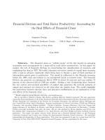
Figure 1: Real Exchange Rate and Real Interest Rate in Mexico
2 Data
Exchange Rates and Interest Rates The main events associated with the Mexican
crisis of 1994 are well documented. On December 20 1994, the government devalued the
peso by 15 percent in response to capital outflows and a run on the currency. When this
proved insufficient to halt capital flight, the peso was allowed to float two days later. Between
1994 and 1995, the real exchange rate depreciated by more than 55 percent.
The left panel of Figure 1 shows the evolution of the multilateral, CPI based, real
exchange rate (peso to the dollar), calculated by the Central Bank of Mexico using a basket
of 118 currencies. The dotted line shows the ratio of the prices in the traded goods sector
to prices in the non-traded goods sector.
6
The increase in this price ratio due to the devalu-
ation was 8 percent, a much smaller magnitude than the 58 percent depreciation of the real
exchange rate. The subsequent trend however, mirrored the behavior of the real exchange
rate and the series edged closer from 1998 onwards.
Interest rates shot up simultaneously. The right panel of the same figure shows a
measure of the domestic interest rate in dollar terms based on the return on 28 day Mexican
6
While the precise definition of a traded or non traded good is sometimes contentious, we define the
traded goods sector as comprising of agriculture, manufacturing and mining, while the non traded goods
sector consists of construction, and all services. The price index of each sector is calculated as the weighted
average of the price indices of all the economic activities encompassed by it. The weights are calculated as
the share of the activity in sectoral value added.
5
treasury bills (CETES).
7
As observed, the interest rate fell steadily from 1988 to 1994, a
period of financial liberalization in Mexico. During the sudden stop it increased to almost
50 percent, from a level of 7 percent in 1994. In 1996 it fell slightly to 30 percent and slowly

declined to pre-crisis levels. This is the change in interest rates that we will use for the crisis
scenario. Its large magnitude reflects not only the perceived risk of default of the Mexican
government
8
but also the quantitative restrictions to borrowing implied by the sudden stop
of foreign capital.
It is hard to get a direct measure of the real cost of short run borrowing for businesses
in Mexico during the crisis, but casual evidence suggests that it was not far off the 50 percent
implied by the ex-post CETES rate in dollars.
9
We also provide in Figure 1 an alternative
measure based on firm level data of (arguably large) Mexican firms listed on the stock market.
We calculate the cost of credit for the median firm as the ratio of the real value of interest
payments to the real value of the stock of bank debt. As observed in the figure, this real
implict interest rate increased from 17 percent in 1994 to 42 percent in 1995, and declined
to 30 percent the year after, very much in line with the ex-post CETES rate in dollars.
Output and TFP The real effects of the devaluation and interest rate hike were imme-
diate. The top left panel of Figure 2 shows that GDP, which had been growing at about 4
percent per annum fell by over 6 percent in 1995. This decline was more pronounced in the
non traded goods sector than in the traded goods sector, as the second and third panels of
the figure show.
Using detrended data on sectoral value added, labor and capital we perform a standard
growth accounting exercise to decompose the fall in GDP in 1995.
10
We use detrended data
7
In our model, all quantities, including the rate of interest will be expressed in terms of the traded good.
The domestic interest rate in terms of dollars is the closest analog to this in the data. Ideally, we would like
to have an ex-ante interest rate in dollars, but the information to construct it is not available. Instead, we
construct an ex-post short run rate as the difference between the interest rate in pesos and the devaluation

rate over the next month.
8
For example, the return on the J.P. Morgan Emerging Markets Bond Index Plus (EMBI+) for Mexico
increased from 5 to 15 percent from 1994 to 1995, and remained close to 10 percent till the end of 1996 (see
Uribe and Yue 2006). This index captures the country specific risk of sovereign default.
9
In April 1995, the New York Times reported that entrepreneurs faced interest rates of over 100%. On
August 24 of the same year the Mexican government announced a $1.1 billion plan to guarentee interest
rates at half their current level. Under the plan, the interest rate on the first $31,400 of business loans would
be reduced from about 60% to 25%.
10
Data for value added and employment comes form INEGI’s national income and product accounts. Data
6
9.1
9.2
9.3
9.4
9.5
9.6
9.7
1988
1989
1990
1991
1992
1993
1994
1995
1996
1997

1998
1999
2000
7.8
7.9
8
8.1
8.2
8.3
8.4
1988
1989
1990
1991
1992
1993
1994
1995
1996
1997
1998
1999
2000
GDP in the Traded Goods Sector
8.8
8.9
9
9.1
9.2
9.3

9.4
9.5
1988
1989
1990
1991
1992
1993
1994
1995
1996
1997
1998
1999
2000
Actual Trend
GDP in the Non Traded Goods Sector Total Factor Productivity
85
90
95
100
105
110
115
1994
1995
1996
1997
1998
1999

2000
Aggregate T Sector N Sector
Aggregate GDP
Figure 2: Output and Total Factor Productivity in Mexico
7
Table 1: Growth Accounting for Mexican Economy - Detrended Variables
Annual Growth Total Traded Non-traded
Rate: 1994-95 Sector Sector
GDP -9.2% -6.3% -10.2%
Capital 0.3% 1.2% -0.6%
Labor -4.8% -4.9% -4.7%
TFP -6.7% -4.4% -7.2%
to abstract from the long run growth rate of the total labor force and productivity, as these
features are absent in our model.
11
Table 1 shows the results. As expected, TFP is the
main driving force behind the output drop both at the economy-wide and sectoral levels,
explaining 73 percent of the overall fall in GDP.
The lower right panel of Figure 2 shows the evolution of aggregate and sectoral de-
trended TFP during and following the Mexican crisis. The immediate collapse in TFP was
higher in the non-traded sector. During the recovery TFP grew at a faster rate in the traded
sector (2.2 percent per year) than in the non-traded sector, where productivity staganated
for the rest of the decade.
Decline in Intermediate Inputs While output fell without a corresponding drop in
measured labor and capital, there was a large decline in the use of intermediate inputs.
From NIPA data, we estimate this fall to be around 4.8 percent in 1995. Moreover, the
consumption of energy, one of the most important intermediate goods, fell by over 10 percent
in this period, as documented by Meza and Quintin (2006).
The use of trade credit, which is typically used to finance intermediate good consump-
tion also fell in this period. While macro data on trade credit is not available, data from

firms listed on the Mexican stock exchange show that as a fraction of short term liabilities,
the stock of trade credit outstanding fell from 24 percent in December 1994 to 20 percent
by the end of 1995. Recovery to pre-crisis levels occurred only by 1997.
for capital stock by sector is obtained from Banco de Mexico surveys. We use the factor shares α
T
= 0.48,
α
N
= 0.36, and α = 0.4. The choice of these values will be discussed in detail in the calibration section.
11
Labor is detrended at the annualized rate of growth of total employment from 1988 to 2002 (n = 0.0195).
Capital and GDP are detrended at the rate (1 + g) (1 + n)−1, where g = 0.0125 corresponds to the annualized
growth rate of per worker GDP in the same period. Finally, TFP is detrended at the rate (1 + g)
1−α
− 1.
We use the same rates to detrend total and sectoral variables.
8
Share in Productive Factors
0.2
0.3
0.4
0.5
0.6
0.7
1988
1989
1990
1991
1992
1993

1994
1995
1996
1997
1998
1999
2000
Labor Capital
Share in Output (GDP)
0.2
0.25
0.3
0.35
1988
1989
1990
1991
1992
1993
1994
1995
1996
1997
1998
1999
2000
Figure 3: Share of Traded Goods in Output, Labor and Capital
Inter-Sectoral Reallocation of Resources Figure 3 shows the share of the traded
goods sector in GDP, labor and capital. In line with the experience of most industrial-
ized economies, the long term process of structural transformation in Mexico saw a decline

in the importance of the traded goods sector as services eclipsed manufacturing in impor-
tance. The large devaluation in 1995, together with the passage of NAFTA the year before,
reversed this trend in output and the share of traded goods in output increased by about
0.8 percent in that year, consistent with the trends for sectoral TFP discussed before.
12
Interestingly, this was not accompanied by a similar increase in the share in labor and
capital. While the pace of the decline in the share of labor slowed, and the share of capital
increased after about two years, no large and immediate reallocation of resources took place,
as a standard frictionless model would predict after the devaluation. This suggests that costs
of adjustment of labor and capital can be important in explaining the response of output in
both sectors.
12
Meza and Urrutia (2010) analyze the long run behavior of the real exchange rate in Mexico and linked
it to this process of structural transformation of the economy, together with a decline in the cost in foreign
borrowing due to financial liberalization.
9
3 The Baseline Model
In this section we set up the baseline model with the financial friction. As mentioned
earlier, the model economy is a small open economy which produces traded and non-traded
goods. Both goods are combined to produce a final good which is consumed and invested.
Traded and non traded goods are also combined to produce the intermediate good used
in their production. In addition, the traded good is exported and used for borrowing and
lending. A representative firm in each sector produces according to a constant returns to
scale production function using capital, labor and intermediate goods.
We introduce the financial friction as a working capital requirement for production. As
in Mendoza and Yue (2009), intermediate goods must be purchased in advance of production
using (short term) borrowing in traded goods.
13
In the small open economy, the interest rate
on these loans is given by the world real interest rate. During the sudden stop, an increase

in interest rates, through its effects on the purchase of intermediate goods, will increase the
cost of production.
A representative consumer supplies labor and rents capital to each sector, demands
final goods, invests in capital goods, and borrows or lends from abroad at the world interest
rate. At each period, all factor and goods markets clear. The price of the final good is the
numeraire. We now describe this economy in detail.
Consumers The representative consumer is endowed with one unit of labor which is sup-
plied inelastically.
14
Each period, the consumer consumes the final good C
t
, saves/borrows
in foreign bonds B
t+1
valued at the price of traded goods p
T
t
, and invests in capital K
t+1
.
The consumers problem can be written as
max
C
t
,K
t+1
,B
t+1
∞


t=0
β
t

C
1−σ
t
− 1
1 − σ

13
Schwartzman (2010) provides evidence that output reallocates from industries with high inventory to
variable cost ratios towards industies with lower ratios in times of interest rate increase, indicating that
holding these inventories in advance of production may be costly.
14
Since our main interest is understanding the movements in TFP and their contribution to a fall in
output, we abstract from variations in factor use as an explanation for a fall in GDP.
10
subject to the budget constraint
C
t
+ K
t+1
+ p
T
t
B
t+1
= w
t

+ [r
t
+ (1 − δ)] K
t
+ (1 + r
∗
t
) p
T
t
B
t
−
ψ
K
2

K
t+1
− K
t
K
t

2
The rental rate on capital is r
t
, and the depreciation rate is δ. The interest rate on bonds is
given by r
∗

t
. The intertemporal costs of adjustment of capital are governed by the parameter
ψ
K
and β is the discount factor.
Final Goods Producers The final good is used for consumption and investment and is
produced using the non-tradable good Q
N
t
and the tradable good Q
T
t
. Each period, the
producer of the final good solves the following problem
max
Q
T
t
,Q
N
t

Y
t
− p
T
t
Q
T
t

− p
N
t
Q
N
t

where the production technology is given by
Y
t
=

γ

Q
T
t

ρ
+ (1 − γ)

Q
N
t

ρ

1
ρ
. (1)

The price of the final good is the numeraire.
Traded and Non traded Goods Producers Traded and non traded goods are produced
domestically by representative firms in each sector i = T, N with a Cobb Douglas production
function
Y
i
t
= A
i
t


K
i
t

α
i

L
i
t

1−α
i

ε
i

M

i
t

1−ε
i
, (2)
using capital, labor L
i
t
and intermediate goods M
i
t
.
Production in this sector is subject to the working capital constraint mentioned earlier.
A fraction κ of the purchase of intermediate goods needs to be financed by within period
loans, at an interest rate r
t+1
. Hence the firm’s problem in the i
th
sector (i = T, N) can be
written as
max
K
i
t
,L
i
t
,M
i

t
p
i
t
Y
i
t
− w
t
L
i
t
− r
t
K
i
t
− p
M
t
(1 − κ) M
i
t
− p
M
t
κ (1 + r
t+1
) M
i

t
11
or equivalently,
max
K
i
t
,L
i
t
,M
i
t
p
i
t
Y
i
t
− w
t
L
i
t
− r
t
K
i
t
− p

M
t
M
i
t
where
p
M
t
= p
M
t
(1 + κr
t+1
) (3)
The loans are supplied by competitive financial intermediaries at an interest rate determined
below.
Financial Intermediary In each period t, firms need to borrow an amount κp
M
t
M
t
, mea-
sured in terms of the domestic final good, where M
t
= M
T
t
+ M
N

t
. The competitive financial
intermediary borrows an equivalent amount from abroad in traded goods, namely
κp
M
t
M
t
p
T
t
at
the interest rate r
∗
t+1
, repayable next period. The firms repay the intermediary the amount
(1 + r
t+1
) κp
M
t
M
t
within the same period t. The intermediary stores this amount, converts it
to traded goods at time t + 1, and returns it to the foreign lender. The zero profit condition
for the intermediaries implies that their costs of funds must equal the amount received from
firms. In other words

1 + r
∗

t+1

κp
M
t
M
t
p
T
t
= (1 + r
t+1
)
κp
M
t
M
t
p
T
t+1
.
which gives us the interest rate
r
t+1
=

1 + r
∗
t+1


p
T
t+1
p
T
t
− 1.
In what follows, we will find it convenient to define the gross real interest rate as
R
t+1
=

1 + r
∗
t+1

p
T
t+1
p
T
t
(4)
Intermediate Goods Producers: The production function for intermediate goods is
given by
M
t
= A
M



M
T
t

φ


M
N
t

1−φ
12
where

M
T
t
and

M
N
t
are the demand for tradable and non-tradable goods used as inputs for
intermediates. The problem of the representative firm can be written as
max
{
M

t
,

M
T
t
,

M
N
t
}
p
M
t
M
t
− p
T
t


M
T
t

− p
N
t



M
N
t

subject to
M
t
= A
M


M
T
t

φ


M
N
t

1−φ
Equilibrium The market clearing conditions for this model are:
(i) for the final good
Y
t
= C
t

+ K
t+1
− (1 − δ) K
t
+
ψ
K
2

K
t+1
− K
t
K
t

2
+ R
t+1
κp
M
t
M
t
− R
t
κp
M
t−1
M

t−1
(5)
The last two terms are included because they represent the amount of final good which the
financial intermediary stores today less the amount stored from the previous period, which
is needed for the repayment of the loans of the last period.
(ii) for tradable and non-tradable goods
Q
T
t
+

M
T
t
+ NX
t
= Y
T
t
Q
N
t
+

M
N
t
= Y
N
t

where NX
t
are net exports.
(iii) for intermediate goods
M
T
t
+ M
N
t
= M
t
and
(iv) for capital and labor
K
T
t
+ K
N
t
= K
t
L
T
t
+ L
N
t
= 1
13

Macroeconomic Aggregates GDP in this economy can be expressed as
GDP
t
= Y
t
+ p
T
t
NX
t
(6)
= p
T
t
Y
T
t
+ p
N
t
Y
N
t
− p
M
t
M
t
(7)
= w

t
+ r
t
K
t
+ (R
t+1
− 1) κp
M
t
M
t
(8)
using the value of final goods, the sum of all value added and the total income in the economy
respectively. The last term in equation (8) is the income of the intermediary in the current
period and is equal to

p
M
t
− p
M
t

M
t
.
The current account balance can be derived by noting that the budget constraint of
the consumer
w

t
+ r
t
K
t
= C
t
+ K
t+1
− (1 − δ) K
t
+
ψ
K
2

K
t+1
− K
t
K
t

2
+ p
T
t
B
t+1
− (1 + r

∗
t
) p
T
t
B
t
can be written as
Y
t
+ p
T
NX
t
− (R
t+1
− 1) κp
M
t
M
t
= Y
t
− R
t+1
κp
M
t
M
t

+ R
t
κp
M
t−1
M
t−1
+ p
T
t
B
t+1
− (1 + r
∗
t
) p
T
t
B
t
by using the equality between equations (6) and (8) on the left hand side and substituting
equation (5) on the right hand side.
This implies that the balance of payments identity is
p
T
t
B
t+1
− (1 + r
∗

t
) p
T
t
B
t
− κp
M
t
M
t
+ R
t
κp
M
t−1
M
t−1
= p
T
t
NX
t
where the net foreign asset position of the country includes not only the stock of foregin
bonds, but also (with a minus sign) the debt position of financial intermediaries.
Given an initial capital stock K
0
and an initial net asset position B
0
, the deterministic

equilibrium in this model is the solution to a system of non linear equations, details of which
are given in Appendix A.
14
3.1 Calibration
We calibrate the model to match key features of the Mexican economy on the eve of the
crisis. To quantify the interactions between sectors, we use the input output tables reported
in Kehoe and Ruhl (2009).
Production Function Parameters For the traded goods sector the following two ratios
suffice to identify production function parameters
Intermediates Consumption
Value Added
=
(1 − ε
T
)
ε
T
= 1.103
Employee Compensation
Value Added
=
(1 − α
T
) ε
T
ε
T
= 0.521.
These two equations give us the values for ε
T

= 0.475 and α
T
= 0.479.
Similarly for the non traded goods sector
Intermediates Consumption
Value Added
=
(1 − ε
N
)
ε
N
= 0.438
Employee Compensation
Value Added
=
(1 − α
N
) ε
N
ε
N
= 0.642,
implying that ε
N
= 0.696 and α
N
= 0.358. Not surprisingly, the traded goods sector is more
capital intensive and uses intermediates more intensively than the non traded goods sector.
Intermediate Goods Production Parameters: To get the parameter φ, i.e. the pro-

portion of traded goods used in the production of intermediate goods, we note that the first
order conditions for the intermediate goods producers imply that
p
T
t

M
T
t
p
N
t

M
N
t
=
φ
1 − φ
.
The counterpart to this in the input output tables is
Traded Goods Used as Intermediates
Non Traded Goods Used as Intermediates
= 1.243,
15
which results in a value of φ = 0.554.
Financial Constraint The fraction of intermediate goods that need to be bought on
credit κ, is a key parameter of the model, since it governs the size of the wedge between the
producer and user cost of intermediate goods. This is calibrated using a combination of firm
level data and macro data. κ can be decomposed as

κ =
Intermediate goods bought on credit
Intermediate Goods
=

Intermediate Goods bought on credit
Output

×

Total Output
Intermediate Goods

The numerator of the first term is hard to estimate. However, from firm level data we have
a measure of short term debt liabilities. Using this data for the numerator and the sum of
total sales and inventories for the denominator gives us the first ratio.
15
The second ratio
comes from the NIPA data and is the ratio of gross output to total intermediate goods. The
product of these ratios gives us a value of κ = 0.7. This is lower than the value of κ = 1
used in Neumeyer and Perri (2005) and Uribe and Yue (2006). However, it is higher than
the 10 percent value used in Mendoza and Yue (2009), who calibrate it to the volatility of
the trade balance. We experiment with a range of values to explore the sensitivity of our
results to this parameter.
16
Utility Function and Final Good Production Parameters We set σ = 2, which is
consistent with an intertemporal elasticity of substitution of consumption of 0.5. Following
Kehoe and Ruhl (2009) and Stockman and Tesar (1995) we set ρ = −1, consistent with an
elasticity of substitution between traded and non traded goods of 0.5. To get γ note that
the first order conditions from the final goods producer problem imply that

p
T
p
N
=
γ
1 − γ

Q
N
Q
T

2
15
The data comes from the Mexican stock market and consists of firms that are listed or have issued
commercial paper in the period 1989-1999.
16
Given parameter values, κ = 0.7 implies a model predicted debt to GDP ratio of about 40% in steady
state. The ratio of non-household private debt to GDP was slightly over 50% in 1994.
16
Relative to a base price ratio, we can identify γ from the ratio of traded goods to non traded
goods used in the production of final goods. Since final goods in our model are used for
consumption and investment, we use the input output table to get
γ
1 − γ
=

Q
T

Q
N

2
=

C
T
+ I
T
C
N
+ I
N

2
= 0.295
which implies a γ of 0.228.
Outside the crisis, the interest rate r
∗
is set to 5%, consistent with average world real
interest rates. The consumer’s discount factor β is set to
1
1+r
∗
.
Parameters calibrated to the steady state The parameters that remain to be charac-
terised are the scale parameters A
T
, A

N
and A
M
. We also need to specify the initial stock
of assets B
0
and the adjustment costs of capital ψ
K
.
We compute a steady state equilibrium for the model economy, and calibrate the values
of A
T
and A
M
and B
0
relative to A
N
, which is set to 1. The goal is to jointly match three
targets, the share of labor in the traded goods sector, the investment to output ratio and the
trade balance in 1994. While we do not claim that the Mexican economy was in a steady
state in 1994, given the appreciating real exchange rate, declining interest rates and the
increasing share of the non traded goods sector in the economy over the five previous years,
calibrating to a steady state or transition is irrelevant for our purposes, except as a means
to get initial conditions for the experiment. We also check the sensitivity of our results to
these initial conditions.
Finally, the adjustment cost parameter ψ
K
is calibrated to match the the investment to
GDP ratio in 1995. The parameters calibrated and the statistics they match are summarized

in Table 2.
3.2 The Experiment
To understand how the economy performs after a sudden stop, we perform the following
experiment. Beginning from a steady state calibrated to match key features of the Mexican
economy in 1994, as described in the previous section, we increase the interest rate, r
∗
t+1
17
Table 2: Calibrated Parameters
Statistic Target Parameter Value
Ratio of T to N final goods 0.295 γ 0.228
Share of Labor in T sector value added 0.521 α
T
0.479
Ratio of intermediates to T sector value added 1.103 ε
T
0.475
Share of Labor in N sector value added 0.642 α
N
0.358
Ratio of intermediates to N sector value added 0.438 ε
N
0.696
Ratio of T to N intermediate goods 1.243 φ 0.554
Fraction of intermediates bought on credit 0.70 κ 0.70
Depreciation Rate δ 0.05
Elasticity of substitution between T and N 0.5 ρ -1.0
Intertemporal elasticity of substitution 0.5 σ 2.0
World Interest Rate 0.05 r
∗

0.05
Fraction of Total Labor in T goods sector 0.35 A
T
1.676
Ratio of Investment to GDP 0.20 A
M
0.126
Ratio of Net Exports to GDP -0.05 B
0
0.020
Investment to GDP Ratio in 1995 0.15 ψ
K
1.15
for two periods, to 50 percent in the first period and 30 percent in the second period, as
observed in the data in Figure 1. The interest rate hike is a perfect surprise to agents, but
once it occurs, they know for how long it will last.
17
TFP and Output Effects As interest rates increase, the wedge between the producer
price and the user price of intermediate goods increases. In our model this is measured as

p
M
t
− p
M
t

= (R
t+1
− 1) κp

M
t
where
R
t+1
= (1 + r
t+1
)
p
T
t+1
p
T
t
Notice that the increase in the wedge comes from two sources: first the increase in the interest
rate itself, and second from the increase in the price of traded goods, as a result of increased
savings. In Appendix B we show analytically, in the context of a simplified model, how
17
Notice that this is not a very important assumption in our model since in the model agents have limited
ability to hedge against the interest rate shock. As Meza and Quintin (2008) and Pratap and Quintin (2010)
show, the only difference between a perfect foresight and a perfect surprise scenario is that in the former the
capital output ratio in the economy, counterfactually, falls before the shock.
18
Net Exports to GDP Ratio
-0.2
-0.1
0.0
0.1
0.2
0.3

1994 1995 1996 1997 1998 1999 2000
Relative Price of Tradable Goods (PT/PN)
80
90
100
110
120
130
140
1994 1995 1996 1997 1998 1999 2000
Real GDP
90
100
110
1994 1995 1996 1997 1998 1999 2000
Model Data

Aggregate TFP
90
100
110
1994 1995 1996 1997 1998 1999 2000
Figure 4: Aggregates in the Baseline Model
changes in interest rate map into changes in TFP when a financial friction for the purchase
of intermediates is present.
The top two panels of figure 4 show that the resulting fall in aggregate TFP and output
is 3.5 percent, accounting for 52 percent of the observed decline in TFP and 74 percent of
output per worker in the data.
18
Since our model does not admit a role for variations in

labor supply, which account for about one third of the decline in GDP in the data (as seen
in Table 1), we compare its predictions to macroeconomic aggregates per worker.
The Real Exchange Rate and Current Account Since the economy saves in traded
goods, the demand for traded goods also goes up as interest rates increase, putting upward
pressure on the relative price of the traded good. The lower left panel of Figure 4 shows the
18
Variables in the data are detrended following the same procedure as in Section 2.
19
model predicted relative price ratio, compared to that in the data. The model predicts an
increase of 9.8 percent, as compared to 8 percent observed in the data. This is short of the
55 percent depreciation of the real exchange rate observed in the data, which is expected
since our model does not allow for deviations in the law of one price for traded goods. As
interest rates come back to their pre-crisis level, the real exchange rate also returns to its
1994 levels. In the data the return was much more gradual.
In addition, the model predicts a current account reversal as the lower right panel in
Figure 4 shows, although it overpredicts the magnitude of the changes. From a deficit of
about 5 percent the current account to GDP ratio increased to a surplus of about 4 percent
in the data and about 10 percent in the model. As the interest rate returns to normal, the
trade balance deteriorates, again, at a faster rate in the model than in the data.
Sectoral Output and the Intersectoral Reallocation of Resources Thus far the
model has performed remarkably well in explaining the behavior of macroeconomic aggre-
gates following the sudden stop. This aggregate picture however, obscures discrepancies at
the sectoral level. The top two panels of figure 5 show the model predicted and the actual
(detrended) GDP per worker in the traded and non traded goods sector respectively. As the
figures make clear, the baseline model contradicts the data in some important dimensions.
The model predicts an increase in the output per worker of the traded goods sector
of almost 10 percent, whereas in the data it declined by about 1.6 percent. It also greatly
over-predicts the decline in the non traded goods sector. The middle panels show the fall in
TFP in each sector generated by the model. Contrary to the data, the model predicts that
TFP fell by much more in the traded goods sector. Despite this fall in TFP, output in the

traded goods sector increases due to a large reallocation of labor and capital from the non
traded to the traded goods sector, following the real depreciation. However the data does
not support the reallocation of productive factors implied by the model.
Clearly if our model is to match the sectoral data, we need to understand the frictions
that impede the reallocation of factors of production. We introduce such frictions in the
following section.
20
Real GDP in T Sector
90
100
110
120
1994 1996 1998 2000
Model Data
Real GDP in the N Sector
85
95
105
115
1994 1995 1996 1997 1998 1999 2000
Year
TFP in the T Sector
90
100
110
120
1994 1995 1996 1997 1998 1999 2000
TFP in the N Sector
90
100

110
120
1994 1995 1996 1997 1998 1999 2000
KT/KN
90
100
110
120
130
1994 1995 1996 1997 1998 1999 2000
Labor Share of T Sector
0.3
0.34
0.38
0.42
1994 1995 1996 1997 1998 1999 2000
Figure 5: Sectoral Patterns in the Baseline Model
21
4 Model with Reallocation Frictions
We introduce two frictions into the baseline model. First, a labor adjustment cost is incurred
if labor moves from one sector to another. For analytical convenience, we assume that this
cost is borne by the consumer.
19
Second, we assume that capital is completely sector specific
and can be augmented only by new investment in that particular sector.
The representative consumer chooses consumption, C
t
, savings B
t+1
, capital stock in

each sector K
T
t+1
and K
N
t+1
,and the fraction of their labor endowment to be supplied to the
traded goods sector θ
t
, to maximize the discounted stream of their lifetime utility subject to
the budget constraint:
C
t
+ K
T
t+1
+ K
N
t+1
+ p
T
t
B
t+1
=
w
T
t
θ
t

+ w
N
t
(1 − θ
t
) +

r
T
t
+ (1 − δ)

K
T
t
+

r
N
t
+ (1 − δ)

K
N
t
+ (1 + r
∗
t
) p
T

t
B
t
−
ψ
K
2

K
T
t+1
− K
T
t
K
T
t

2
−
ψ
K
2

K
N
t+1
− K
N
t

K
N
t

2
−
ψ
L
2
(θ
t
− θ
t−1
)
2
The parameter ψ
L
controls the adjustment cost of labor. We do not take a stand on whether
this cost reflects human capital losses due to sector specific skills, the cost of unemploy-
ment spells or deadweight losses incurred by firms in their firing and hiring decisions. Our
quadratic adjustment cost function should be seeing as a reduced form encompassing different
possible stories.
Note that the labor market friction and the capital specificity imply that factor prices
do not equate across each sector and are now sector specific as well. As documented in
Meza and Urrutia (2010), changes in the relative wage of workers in the traded and non-
traded goods sectors have been important in Mexico during the 1988-2002 period, reflecting
systematic deviations from sectoral wage equalization.
19
Pratap and Quintin (2010) show that workers who change occupations during the crisis in Mexico saw
their wages fall by about 10% more than those who did not move, even after controlling for observed and

unobserved characteristics.
22
Real GDP
90
95
100
105
1994 1995 1996 1997 1998 1999 2000
Model Data

Total Factor Productivity
90
95
100
105
1994 1995 1996 1997 1998 1999 2000
Figure 6: Aggregates in the Augmented Model
The rest of the model is the same as before, including the financial friction for pur-
chasing intermediate goods. The market clearing equations for the final good is now
Y
t
= C
t
+ K
t+1
− (1 − δ) K
t
+
ψ
K

2

K
T
t+1
− K
T
t
K
T
t

2
+
ψ
K
2

K
N
t+1
− K
N
t
K
N
t

2
+

ψ
L
2
(θ
t
− θ
t−1
)
2
+ R
t+1
κp
M
t
M
t
− R
t
κp
M
t−1
M
t−1
where K
t
= K
T
t
+ K
N

t
, L
T
t
= θ
t
and L
N
t
= (1 − θ
t
).
4.1 Calibration and Experiment
As in the previous section, we compute the steady state equilibrium and choose parameters
to match the Mexican economy in 1994. All parameters are calibrated as described in the
previous section. In addition, the labor adjustment parameter ψ
L
is calibrated to deliver the
labor share of the traded goods sector in 1995. We perform the same experiment as before
where interest rates are unexpectedly increased for two periods.
The aggregate effects of the sudden stop are shown in Figures 6. Aggregate output
and TFP per worker falls by 2.5 percent, compared to 3.5 percent in the case without labor
and capital frictions. This accounts for more than half of the fall in output per worker and
a third of the fall in TFP. Somewhat counterintuitively, the reallocation frictions actually
23
mitigate the misallocation of resources engendered by the financial friction. This is because
of the rate of growth of the price of tradable goods, which enters in the definition of the
gross interest rate which governs the size of the wedge between the producer and user cost
of intermediate goods:
R

t+1
= (1 + r
t+1
)
p
T
t+1
p
T
t
With allocative frictions, the price of the traded goods overshoots in the period where the
interest rate shock occur, but then comes back more gradually to its initial level, as sectoral
output adjusts to meet the initial change in sectoral demand.This implies smaller values for
the wedge and therefore less misallocation due to financial frictions.
Unlike the previous model, this aggregate drop in output is consistent with sectoral
patterns, as shown in Figure 7. The assumption of capital specificity ensures that no capital
is immediately reallocated after the sudden stop. Labor too, does not move immediately
from the non traded goods sector to the traded goods sector. The model predicts a fall of
about 1.4 percent in GDP per worker in the traded goods sector, and a 3.4 percent fall in
the non traded goods sector, accounting for almost 90 percent of the former and more than
half (57 percent) of the latter. TFP also fell in both sectors, more in the non traded, than
in the traded goods sector.
We see therefore that our model augmented with labor market frictions and capital
specificity can account for about 40 percent of the decline in TFP and more than half
the fall in aggregate output per worker. In addition, it is consistent with the patterns of
reallocation of labor and capital observed in the data, as well as the sectoral composition of
output.
It is worth mentioning that since our main interest is in capturing the behaviour of
the economy in the immediate aftermath of the crisis, neither the model nor the experiment
has been designed to account for the recovery in GDP that took place after two years. The

recovery can be attributed to a sustained increase in TFP in the traded goods sector, as
shown in Figure 2, which is likely a result of structural reforms and a fall in tariffs related
to trade liberalization. In our model the only way for TFP to increase is through a fall in
interest rates. In the experiment interest rates come back to their pre-crisis levels after two
24
Real GDP in T Sector
90
100
110
120
1994 1995 1996 1997 1998 1999 2000
Model Data
Real GDP in the N Sector
90
100
110
1994 1995 1996 1997 1998 1999 2000
TFP in T Sector
90
100
110
120
1994 1995 1996 1997 1998 1999 2000
TFP in the N Sector
90
100
110
1994 1995 1996 1997 1998 1999 2000
Labor Share of T Sector
0.3

0.35
0.4
1994 1995 1996 1997 1998 1999 2000
Ratio of (KT/KN)
80
100
120
140
1994 1995 1996 1997 1998 1999 2000
Figure 7: Sectoral Patterns in the Augmented Model
25