Accident Precursor Analysis And Management ppt
Bạn đang xem bản rút gọn của tài liệu. Xem và tải ngay bản đầy đủ của tài liệu tại đây (434.03 KB, 40 trang )
Advances: Engineering Risk Analysis Page 1 of 40 Ch 16 060502 V04
16 The Engineering Risk Analysis Method and Some Applications
M. Elisabeth Paté-Cornell
ABSTRACT
Engineering risk analysis methods, based on systems analysis and probability, are generally
designed for cases in which sufficient failure statistics are unavailable. These methods can be
applied not only to engineered systems that fail (e.g., new spacecraft or medical devices), but
also to systems characterized by performance scenarios including malfunctions or threats. I
describe some of the challenges in the use of risk analysis tools, mainly in problem formulation,
when technical, human and organizational factors need to be integrated. This discussion is
illustrated by four cases: ship grounding due to loss of propulsion, space shuttle loss caused by
tile failure, patient risks in anesthesia, and the risks of terrorist attacks on the US. I show how the
analytical challenges can be met by the choice of modeling tools and the search for relevant
information, including not only statistics but also a deep understanding of how the system works
and can fail, and how failures can be anticipated and prevented. This type of analysis requires
both imagination and a logical, rational approach. It is key to pro-active risk management and
effective ranking of risk reduction measures when statistical data are not directly available and
resources are limited.
Advances: Engineering Risk Analysis Page 2 of 40 Ch 16 060502 V04
CONTENTS
Engineering Risk Analysis Method: Imagination and Rationality
Pro-Active Risk Management
Early Technology Assessment and Anticipation of “Perfect Storms”
Remembering the Past While Looking Ahead
A Brief Overview of the Method and Formulation Challenges
The Challenge of Structuring the Model
Dynamic Analysis
Imagination and Rationality
Incomplete Evidence Base
Data
The Tool Kit
Extension of RA to Include Human and Management Factors: The SAM Model
Example 1. Ship Grounding Risk: Influence Diagram and SAM Model Representation
The Grounding of Oil Tankers or Other Cargo Ships
Problem Formulation Based on a SAM-Type Influence Diagram
The Overall Risk Analysis Model
Example 2. A Two-Dimensional Risk Analysis Model: The Heat Shield of the Space Shuttle
Orbiters
Example 3. A Dynamic Analysis of Accident Sequences: Anesthesia Patient Risk
Example 4. Probabilistic Analysis of Threats of Terrorist Attacks
Conclusions
Advances: Engineering Risk Analysis Page 3 of 40 Ch 16 060502 V04
Engineering Risk Analysis Method: Imagination and Rationality
Risk analysis for well known, well documented and steady-state systems (or stable phenomena)
can be performed by methods of statistical analysis of available data. These include, for example,
maximum likelihood estimations, and analyses of variance and correlations. More generally,
these methods require a projection in the future of risk estimates based on a sufficient sample, of
preferably independent, identically distributed data, and other experiences from the past.
However, when designing or operating a new type of engineered system, one can seldom rely on
such a body of evidence, even though there may exist relevant data regarding parts of the system
or the problem. The same is true in all new situations in which the risk can only be evaluated
from a rigorous and systematic analysis of possible scenarios, and from dependencies among
events in a scenario. For instance, assessing the risk of a terrorist attack on the US requires
“imagination” as emphasized in the 9/11 Commission Report (NCTA, 2004). To do so, one has
to rely first on a system’s analysis, and second, on Bayesian probability and statistics (e.g.,
Savage, 1954; Press, 1989). The engineering method of “Probabilistic Risk Analysis” (PRA or
here, simply RA), which was designed in the nuclear power industry among other fields
(USNRC, 1975; Henley and Kumamoto, 1992; Bedford and Cooke, 2001), was presented in the
previous chapter
1
. In what follows, I describe some specific features and applications of the
engineering risk analysis method with the objective of finding and fixing system weaknesses,
whether technical or organizational
2
(Paté-Cornell, 2000, 2002a). The focus is mostly on the
formulation phase of a risk analysis, which can present major challenges. I describe and illustrate
four specific problems and possible solutions: the explicit inclusion of human and management
factors in the assessment of technical failure risks using influence diagrams
3
, with as an
Advances: Engineering Risk Analysis Page 4 of 40 Ch 16 060502 V04
example, the case of ship grounding due to loss of propulsion; the characterization of the
dynamics of accident sequences illustrated by a model of analysis of patient risk in anesthesia;
the treatment of spatially-distributed risks with a model of the risk of an accident caused by a
failure of the tiles of the NASA space shuttle; and the challenge of structuring the modeling of a
type of threat that is new –at least on the scale that has been recently observed– illustrated by the
risks of different types of terrorist attacks on the US.
Pro-Active Risk Management
Early Technology Assessment And Anticipation Of “Perfect Storms”
The risk analysis (RA) method used in engineering is based both on systems analysis and
probability and allows computation of the risk of system failure under normal or abnormal
operating circumstances
4
. More importantly, it permits addressing and computing the risk of
“perfect storms”, i.e., rare conjunctions of events, some of which may not have happened yet
even though some of their elements may have been observed in the past. These events can affect,
for instance, the performance of a new space system faced with a combination of challenges
(e.g., a long voyage, cosmic rays, planetary storms, etc.). The same method can be used to
perform early technology assessment, which is especially critical in the development of systems
such as medical devices, which are expensive to engineer and less likely than not to pass the
statistical tests required by the USFDA before approval (Pietzsch et al., 2004). In that context,
RA can thus be used to anticipate the effectiveness and the safety of a new medical device when
the practitioners may not be accustomed to it, when there may be some design problems, and/or
Advances: Engineering Risk Analysis Page 5 of 40 Ch 16 060502 V04
when the patients happen to be particularly vulnerable (e.g., premature babies). In a different
setting, one can also use this type of analysis to assess the risks of combined factors on a firm’s
bottom line, for example, a competitor’s move, a labor strike that affects its supply chain, and/or
a dip in demand caused by a major political event. In that perspective, RA can be applied, for
instance to the quantification of the risks of bankruptcy in the insurance industry when a
company is faced with a decline in market returns, repeated catastrophes, and prosecution of its
executives for professional misconduct (Paté-Cornell and Deleris, 2005). Also, as described
further, the same RA method can be used to support the choice of counter-terrorism measures,
given the limited information provided by the intelligence community, in the face of ever-
changing situations (Paté-Cornell, 2002b).
Remembering the Past While Looking Ahead
Anticipating rare failures, as well as shedding light on mundane but unrecognized problems, can
provide effective support for risk management. But there is a clear difference between
probabilistic risk analysis and expected-utility decision analysis (e.g., Raiffa, 1968), in which the
decision makers are known at the onset of the exercise (Paté-Cornell, 2006). The risk analysis
question is often: what are the risks (as assessed by an analyst and a group of experts), and how
can the results be formulated to best represent uncertainties and be useful to the eventual
decision maker(s)?
The key issue, in all cases, is to anticipate problems that may or may not have occurred
before, and to recognize existing ones in order to devise pro-active risk management strategies.
The engineering risk analysis method permits ranking risk management options and setting
priorities in the use of resources. The quantification of each part of the problem by probability
Advances: Engineering Risk Analysis Page 6 of 40 Ch 16 060502 V04
and consequence estimates allows their combination in a structured way, using both Bayes’
theorem (to compute the probability of various scenarios) and the total probability theorem (to
compute the overall probability of total or partial failures). Effective risk management options
can then be formulated. They include for instance, adding redundancies, but also, the observation
of precursors, i.e., signals and near-misses, which permit anticipating future problems and
implementing pro-active measures (Phimister et al., 2004).
A Brief Overview of the Method and Formulation Challenges
The Challenge of Structuring the Model
The first step in a risk analysis is to structure the future possible events into classes of scenarios
5
as a set of mutually exclusive and collectively exhaustive elements, discrete or continuous. Each
of these scenarios is a conjunction of events leading to a particular outcome. The choice of the
model structure, level of detail, and depth of analysis is critical: as one adds more details to a
scenario description (A and B and C etc.), its probability decreases. In the limit, the exact
realization of a scenario in a continuous space would have a zero probability, making the
exercise useless. Therefore, one needs first to formulate the model at a level of detail that is
manageable, yet sufficient to identify and characterize the most important risk reduction options.
This level of detail may vary from one subsystem to the next. Second, one needs to compute the
probability of the outcomes that can result from each class of scenarios, adjusting the level of
detail, as shown later, to reflect the value of the information of the corresponding variables as
support for risk management decisions. Finally, one needs to quantify the outcomes of these
scenarios and to aggregate the results, sometimes as a probability distribution for a single
Advances: Engineering Risk Analysis Page 7 of 40 Ch 16 060502 V04
attribute (e.g., money), displayed as a single risk curve (e.g., the complementary cumulative
distribution of annual amounts of potential damage); or as the joint distribution of several
attributes of the outcome space
6
(e.g., human casualties and financial losses). To represent the
fundamental uncertainties about the phenomenon of interest, one can display a family of risk
curves, which represent a discretization of the distribution of the probability (or future
frequency) of exceeding given levels of losses per time unit (Helton, 1994; Paté-Cornell, 1996,
1999b).
One can thus represent accident scenarios in various ways. The first is simply accident
sequences, starting with initiating events followed by a set of intermediate events leading to an
outcome described either by a single measure (e.g., monetary) or by a multi-attribute vector. The
distribution of these outcomes allows representation of the risk at various levels of failure
severity. Another analytical structure is to identify “failure modes” or min-cut sets, i.e., the
conjunctions (without notion of sequencing) of events that lead to system failure described as a
Boolean variable (USNRC, 1975). These failure modes account for the structure of the system,
e.g., the fact that the failure of a redundant subsystem requires failure of all its components.
To model the risk using the accident sequence approach, note p(X) the probability of an
event per time unit (or operation), p(X|Y) the conditional probability of X given Y, p(X,Y) the
joint probability of X and Y, IE
i
the possible initiating events of accident sequences indexed in i,
and F the (total
7
) technical failure of the system. In its simplest form, one can represent the result
of the PRA model as the probability p(F) of a system failure per time unit or operation as:
p(F) = Σ
i
(p(IE
i
) x p(F|IE
i
) (1)
Advances: Engineering Risk Analysis Page 8 of 40 Ch 16 060502 V04
where p(F|IE
i
) can be computed as a function of the conditional probabilities of the
(intermediate) events that follow IE
i
and lead to F. The accident sequences can be systematically
represented, for instance through event trees and influence diagrams.
Alternatively, one can start from the system’s failure modes. Noting M
j
these
conjunctions of events (min-cut sets), one can write the probability of failure p(F) using the total
probability theorem as:
p(F) = Σ
j
p(M
j
) – Σ
j
Σ
k
p(M
j
, M
k
) + p (three failure modes at a time) – etc. (2)
External events that can affect all failure modes (e.g., earthquakes) or the probabilities of
specific events in an accident sequence can be introduced in the analysis at that stage. The
method is to condition the terms of the equation(s) on the occurrence (or not) of the common
cause of failure and its severity level.
The choice of one form or another (sequences vs. failure modes) depends on the structure
of the available information. In the ship grounding risk analysis model and the risk analysis of a
shuttle accident presented later, the accident-sequence structure was chosen because it was the
easiest way to think systematically through a collectively exhaustive and mutually exclusive set
of failure scenarios. However, faced with a complex system, best described by its functions and
by a functional diagram, focusing on the failure modes might be an easier choice.
Dynamic Analysis
The robustness of a system as well as the challenges to which it is subjected may change
over time. A structure fails when the loads exceed its capacity. On the one hand, one may want
to account for the long-term pattern of occurrences of the loads (e.g., earthquakes), as well as the
short-term dynamics of the different ways in which such events can unfold, for example, the
Advances: Engineering Risk Analysis Page 9 of 40 Ch 16 060502 V04
time-dependent characteristics of the pre-shocks, main shock and aftershocks of an earthquake
that can hit a structure. On the other hand the system’s capacity may vary as well. It can
deteriorate independently from the loads (e.g., by corrosion), or it can decrease because of the
fatigue caused by repeated load cycles (e.g., the effect of the waves on a structure at sea).
Accounting for variations of loads and capacities requires a knowledge base that may come from
different domains, e.g., from geophysics to structural engineering in the case of seismic risks.
Another form of dynamic analysis may be required to analyze the evolution of accident
sequences in which the consequences depend on the time elapsed between the initiating event
and the conclusion of an incident. This is the case of an analysis of risks of fires in oil refineries
(Paté-Cornell,1985) as well as that of patient risks in anesthesia described further. In both cases,
stochastic processes were used to describe the evolution of the system over time, which is needed
when the timing of human intervention is essential to effective risk management.
Imagination and Rationality
This RA method has been developed in details in the past for specific cases such as
electrical circuits, civil engineering systems, nuclear reactors, aircraft, and space systems. But in
its principles, RA as shown further, has applications to many other problems for which one needs
to “imagine” systematically, beyond a simple, arbitrary “what-if” exercise, the potential failures
in absence of directly relevant experience. In these cases, the choice of evidence is critical
because available information may be incomplete and imperfect, yet essential to support a
rational decision that needs to be made, before the occurrence of an event such as a specified
type of terrorist attack or before a medical device is used in a real setting.
Advances: Engineering Risk Analysis Page 10 of 40 Ch 16 060502 V04
Imagination and rationality are thus two main bases of the PRA method. Risk analysis is
meant to support risk management decisions, assuming a rational decision maker or a
homogenous group of them
8
. Rationality is defined here by the von Neumann axioms of decision
making (von Neumann and Morgenstern, 1947), and by the definition of probability that they
imply
9
. This Bayesian definition differ from the classical frequentist approach in that it relies on
a degree of belief based on a decision maker’s willingness to make bets and to choose among
lotteries given all available evidence. Therefore, by definition, this kind of probability cannot be
“validated” in the classical statistical sense, at least not until one has gathered a sufficient body
of experimental data, and provided that the system has remained in a steady state. This is rarely
the case in innovative engineering or policy making. Instead, one has to seek justification of the
model through a careful presentation of assumptions, reasoning, data and conclusions.
Incomplete Evidence Base
The Bayesian RA method is thus at the root of evidence-based decisions
10
, but this does
not necessarily imply that the evidence involves a complete set of classic statistical data. Again,
this is true because one often has to make such decisions in the face of uncertainty (e.g., in
medicine or in astronautics) before complete information can be obtained. Therefore, the method
uses all the evidence that exists, imperfect as it may be when needed, as opposed to the “perfect”
one that one would want to have to follow the classic statistics path. In effect, the inputs of the
RA method, i.e., the best information available, may be subjective and imperfect, but it may be
the best one has and the process by which the output is generated is a rigorous one.
Since one often needs to use the concept of Bayesian probability based on a degree of
belief, the first question is, of course: whose beliefs? At the onset of a risk analysis, the identity
Advances: Engineering Risk Analysis Page 11 of 40 Ch 16 060502 V04
of the ultimate decision maker is seldom known, it may vary over time, along with the number of
incidents, operations, systems, years of operation. Yet, the results have to be complete enough to
provide information relevant to decision support under various levels of uncertainties when the
event of interest can repeat itself. This implies, in particular that one needs to separate what has
been traditionally referred to as “risk” and “uncertainty” but is better described as two kinds of
uncertainties, “aleatory”, i.e., randomness, and “epistemic”, i.e., incomplete information about
the fundamental phenomenon of interest (Apostolakis, 1990). At the end of the analysis, the
probability of an event, in the face of epistemic uncertainty, is the mean future frequency of that
event, a measure that is compatible with the maximization of expected utility
11
. As shown
further, however, one needs to quantify and fully describe uncertainties about probabilities of
various outcomes to allow decision makers to use the risk results in the case of repeated
“experiments”.
Data
The data that are used in risk analysis thus cover a wide range of sources. In the best of
all worlds, one has access to operational data that describe a particular system or phenomenon in
its actual setting, e.g., flight data for a space system, or steady-state operating room statistics for
a well-known form of surgery. More often, however, in innovative circumstances, one has, at
best, surrogate data regarding performance of subsystems and components in a different but
similar environment. Other times, one may have to use test data and lab data (e.g., on human
performance on simulators). The problem is that tests may have to be performed in an
environment that cannot exactly represent the operational one, for instance micro-gravity for
spacecraft. When one knows the characteristics of the loads to which the system will be
Advances: Engineering Risk Analysis Page 12 of 40 Ch 16 060502 V04
subjected and the factors that influence its capacity, one can also use engineering models as a
source of information. Finally, when facing new situation with no access to such data, in a first
iteration of an analysis, or to supplement existing data, one may need to use expert opinions,
provided that the questions have been phrased in such a way that the experts can actually respond
based on their experience. Biases in these responses have been widely documented and require
all the care of the analyst (e.g., Kahneman et al., 1982). Next, one often faces the unavoidable
challenge of aggregating experts opinions, which is easier when the decision maker is known and
can inject his own “weighting” (in effect, the equivalent of likelihood functions) in the exercise,
and more complex when the risk analysis has to be performed for unknown decisions and
decision makers
12
.
The Tool Kit
The tools of RA thus include all those that allow description of the problem structure and
computation of failure probabilities, in a world that is either static or dynamic. They involve
event trees, fault trees, influence diagrams, Bayesian probability and descriptive statistics
13
, but
also stochastic processes of various sorts depending on the system’s memory, time dependencies
etc. They also include characterization of human errors and of the outcomes of the various
scenarios based, for example, on economic analysis. When expanded to the analysis of risk
management decisions, the tool kit includes decision trees (and the corresponding version of
influence diagrams) and utility functions, single or multi-attribute (Keeney and Raiffa, 1976).
Simulation is often needed to propagate uncertainties through the model in order to link
uncertainties in the input and those in the output. To do so, one can then use for instance, Monte
Advances: Engineering Risk Analysis Page 13 of 40 Ch 16 060502 V04
Carlo simulation, or often better, the Latin Hypercube method, which is based on a similar
approach but allows for a more efficient search.
Extension of RA to Include Human and Management Factors: The SAM Model
Most of the classic risk analyses do include human reliability in one form or another. Human
errors may be included in failures or accident scenarios as basic events, or part of the data of
component failures. Yet, they are not necessarily an explicit part of a scenario, and often simply
weaken a component, e.g., through poor maintenance, which increases a component’s
vulnerability. In addition, human errors are often based on management problems, for example,
wrong incentives, lack of knowledge on the part of the technicians, or excessive resource
constraints.
To address these problems, a model called SAM was devised (Murphy and Paté-Cornell,
1996) based first, on an analysis of the system’s failure risk (S). The second level, involves a
systematic identification and probabilistic characterization of the human decisions and actions
(A) that influence the probabilities of the basic events of the model. Finally, a third level
represents the management factors (M) that in turn, affect the probabilities of the human
decisions and actions
14
.
The main characteristic of the SAM model is thus that it starts with an analysis of the
performance of the physical system. This model can be represented by a three-tier influence
diagram (see Figure 16.1), in which the influences run from the top to the bottom but the analysis
is performed from the bottom to the top. The equations of the SAM model can be described
using the notations of Equations 1 and 2, and in addition, noting as p(L
h
) the probability of the
different loss levels L
h
associated with various degrees of technical system failure indexed in h,
Advances: Engineering Risk Analysis Page 14 of 40 Ch 16 060502 V04
(DA
m
) the probabilities of the decisions and actions of the different actors, and MN
n
the
relevant management factors that affect peoples decisions and actions.
Level 1
Initiating
Event #1
Initiating
Event #2
I
ntermediate
Event #1
I
ntermediate
Event #2
Outcomes
(e.g., Failure
or Loss Levels)
Decision 1
Decision 2
MANAGEMENT
SYSTEM
DECISIONS
AND ACTIONS
PROBABILISTIC
RISK ANALYSIS
Level 2
Level 3
Management
Factor #1
Management
Factor #2
Figure 16.1: Generic influence Diagram representing the structure of the SAM Model.
The SAM equations are:
SAM step 1: probability of system failures characterized by levels of losses:
p(L
h
) = Σ
i
(p(IE
i
) x p(L
h
|IE
i
) (3)
SAM step 2: effects of human decisions and actions on p(losses)
p(L
h
) = Σ
i
Σ
m
p(DA
m
) x p(IE
i
|DA
m
) x p(L
h
|IE
i,
DA
m
) (4)
SAM step 3: effects of management factors on p(losses)
Advances: Engineering Risk Analysis Page 15 of 40 Ch 16 060502 V04
p(L
h
|MN
n
) = Σ
i
Σ
m
p(DA
m
|MN
n
) x p(IE
i
|DA
m
) x p(L
h
|IE
i,
DA
m
) (5)
Note that the effects of management factors on the probabilities of losses are assessed
through their effects on the probabilities of the decisions and actions of the people involved.
Also, we assume here, for simplicity, that the different decisions and actions are mutually
independent conditional on management factors (which can be easily modified if needed).
In what follows, we present four examples of risk analyses, some at the formulation stage
and some with results that include identification of possible risk management options, to
illustrate different features of the RA model and, in three cases, of its SAM extension.
Example 1. Ship grounding risk: Influence diagram and SAM model representation
The Grounding of Oil Tankers or Other Cargo Ships
The experience with the grounding of the Exxon Valdez in Alaska as well as the breaking at sea
of several oil tankers and cargo ships such as the AMOCO-Cadiz off the coasts of Europe, posed
some serious risk management problems. Are the best solutions technical, e.g., requiring double
hulls, or essentially managerial and regulatory in nature, for instance, increased regulation of
maritime traffic and Coast Guard surveillance and/or improvements of the training of the crew?
In some cases, one could even imagine drastic options such as blowing up rocks that are too
close to shipping lanes. Obviously, the risk depends, among other factors, on the nature of the
ship and its cargo, on the skills of its crew, and on the location of maritime routes. Some areas
such as the Molucca Strait are particularly dangerous because of the density of international
traffic and at times, the anarchic or criminal behavior of the crews. Other sites are especially
Advances: Engineering Risk Analysis Page 16 of 40 Ch 16 060502 V04
vulnerable because of their configuration such as Puget Sound, the San Francisco Bay, or Prince
William Sound.
Problem Formulation Based on a SAM-Type Influence Diagram
An analysis of the risks of oil spills due to ship grounding following loss of propulsion
can be represented by an influence diagram, expanded to include human and management factors
in the SAM format. To support a spectrum of risk management decisions, that diagram can be
structured as shown in Figure 2 to include the elements of Figure 1. It represents the sequence of
events starting with loss of propulsion, that can lead to a breach in the hull and in the case of oil
tankers, release of various quantities of oil in the sea, and possibly, sinking of the ship
Advances: Engineering Risk Analysis Page 17 of 40 Ch 16 060502 V04
Loss of
Propulsion
LP
Uncontrolled/
Controlled
Drift
Grounding
Final
System
State
e.g., breach
in tank?
Location
Speed
Weather
Skill level
of the Captain
and the crew
Maintenance
Quality
Personnel
Management
Resource
Constraints
(time and budget)
MANAGEMENT LEVEL
HUMAN DECISIONS AND ACTIONS
PROBABILISTIC RISK
ANALYSIS
Level 3
Level 2
Level 1
Source
Term:
Oil
Flow
Figure 16.2: Influence diagram for the risk of grounding of an oil tanker.
The lower part of Figure 16.2 represents the system’s failure risk analysis model. The
accident sequence starts with the loss of propulsion at sea (initiating event). Given that this event
has happened, the second event is drift control: can the crew control the drift? If not the next
event is grounding of the ship: does it happen or not given the speed, the location and the
weather? If grounding occurs, the next question is: what is the size of the breach in the hull? It
depends on the nature of the seabed or the coast (sand, rocks etc.), on the characteristics of the
hull, and on the energy of the shock. Finally, given the size of the breach, the next question is:
what is the amount of oil spilled in the water? This outcome depends on the amount of oil carried
Advances: Engineering Risk Analysis Page 18 of 40 Ch 16 060502 V04
in the first place and on the size of the breach as well as the external response to the incident.
The final outcome can then be characterized by the financial loss and the environmental damage
measured, for instance, in terms of number animals or length of coastline affected, or in terms of
time to full recovery.
The middle and upper parts of Figure 16.2 represent the decisions, actions, and
organizational roots of the elements of the accident sequence represented in the lower part of the
figure. The failure of a ship’s propulsion system starts with its design, but more importantly in
operations, with inspection and maintenance procedures. The performance of the crew in an
emergency and its ability to prevent grounding depend not only on the skills of its captain but
also on the experience of the sailors, and on the ability of the group to work together and to
communicate, especially in an emergency. The decisions and actions of the crew may thus
depend in turn, on decisions made by the managers of the shipping company who may have
restricted maintenance resources, hired a crew without proper training, and forced a demanding
schedule that did not allow for inspection and repair when needed. The decisions and actions of
crews are treated here as random events and variables conditional on a particular management
system. In this example, the evidence base includes mostly statistics of the frequency of loss of
propulsion for the kind of ship and propulsion system considered and on expert opinions.
The Overall Risk Analysis Model
Based on the influence diagram shown in Figure 2, one can construct a simple risk
analysis model represented by a few equations. Note LP (or not: NLP) the event loss of
propulsion, and p(LP) its probability per operation; CD (or not: UD) the control of the drift, G
(or not: NG) the grounding of the ship; B the random variable for the “final system state” i.e., the
Advances: Engineering Risk Analysis Page 19 of 40 Ch 16 060502 V04
size of the breach in the hull characterized by its probability density function given grounding
f
B
(b|G); and O (random variable) the “source term”, here, the quantity of oil released
characterized by its probability density function f
O
(o), and by its conditional probability density
function f
O|B
(o|b) given the size of the breach in the hull. Grounding can occur with or without
drift control. Using a simple Bayesian expansion, the PRA model can then be written as one
overall equation to represent this particular failure mode :
B
15
f
O
(o) = ∫
b
p(LP)x {p(UD|LP)x p(G|UD)+p(CD|LP)x p(G|CD)}x f
B
(b|G)x f
O|B
(o|b)db (6) B
Given a total budget constraint (management decision), the maintenance quality can be
represented by the frequency and the duration of maintenance operations (e.g., at three levels).
Given the management policy regarding personnel, the experience of the crew can be represented
by the number of years of experience of the skipper (on the considered type of ship) and/or by
the number of voyages of the crew together
16
. These factors, in turn, can be linked to different
probabilities of loss of propulsion, and to the probability of drift control given loss of propulsion,
using expert opinions or statistical analysis.
Numerical data need to be gathered for a specific site and ship, and the model can then be
used to compute the probability distribution of the benefits of different types of risk reduction
measures. For instance, improving maintenance procedures would decrease the probability of
propulsion failure in the first place. Requiring a double hull would reduce the size of the breach
given the energy of the shock. Effective control of the speed of the ship would reduce also the
energy of the shock in case of grounding. Quick and effective response procedures would limit
the amount of oil spilled given the size of the breach in the hull. The model can then be used as
part of a decision analysis. This next step, however, also requires a decision criterion, e.g., what
level of probability of grounding or an oil spill can be tolerated in the area, or, for a specified
Advances: Engineering Risk Analysis Page 20 of 40 Ch 16 060502 V04
decision maker, his or her disutility for the outcomes, including both financial factors and
environmental effects in a single- or multi-attribute utility function.
Example 2. A Two-Dimensional Risk Analysis Model: The Heat Shield of the Space Shuttle
Orbiters
In a study of the tiles of the space shuttle’s heat shield, funded by NASA between 1988 and
1990, the problem was to determine first, what were the most risk-critical tiles, second, what
were their contributions to the overall risk of a mission failure, and third, what were the risk
management options, both technical and organizational that could be considered (Paté-Cornell
and Fischbeck, 1993a, 1993b). The challenge was to formulate the problem of the risk of tile
debonding and of a “burnthrough” for each tile given its location on the aluminum surface of the
orbiter, considering that they are all different, subjected to various loads, and that they cover
areas of varying criticality.
The key to the formulation was first to determine the nature of the accident sequences,
and the way they could unfold. A first tile could debond either because of poor bonding in
installation or during maintenance, or because it is hit by a piece of debris. In turn, adjacent tiles
could come off under aerodynamic forces and the heat generated by turbulent flows in the empty
cavity. Given the size and the location of the resulting gap in the heat shield, the aluminum could
then melt, exposing to hot gases the subsystems under the orbiter’s skin. These subsystems, in
turn, could fail and depending on their criticality, cause a loss of the orbiter and the crew.
Therefore, faced with about 25,000 different tiles on each orbiter, the challenge was to structure
the model to include the most important risk factors, whose values vary across the surface:
aerodynamic forces, heat loads, density of debris hits and criticality of the subsystems under the
Advances: Engineering Risk Analysis Page 21 of 40 Ch 16 060502 V04
orbiter’s skin in different locations. The solution was to divide the orbiter’s surface into areas in
which the values of these factors were roughly in the same range and to represent this partition
on a two-dimensional map of the orbiter
17
. Figure 16.3 is an influence diagram representing the
structure of the model.
Figure 16.3: Influence diagram for an analysis of the risk of an accident caused by the failure of
tiles of the space shuttle. Source: Paté-Cornell and Fischbeck, 1993a.
Data were gathered from both NASA and its main contractors. Figure 16.4 shows the
result of the analysis, i.e., the risk criticality of each tile in different zones (represented by
various shades of grey) as measured by its contribution to the probability of mission failure. The
main results were that tile failures contributed about 10% of the overall probability of a shuttle
accident, and that 15% of the tiles contributed about 85% of the risk.
Advances: Engineering Risk Analysis Page 22 of 40 Ch 16 060502 V04
.
Figure 16.4 Map of the risk criticality of the tiles on the space shuttle orbiter as a function of
their location. Source: Paté-Cornell and Fischbeck, 1993a.
The recommendations to NASA, at the end of the study, were to decrease the time
pressure on the maintenance crews, prioritize inspection, and improve the bonding of the
insulation of the external tank. Some of them were adopted (e.g., reduction of the time
Advances: Engineering Risk Analysis Page 23 of 40 Ch 16 060502 V04
pressures), others not (e.g., improvements of the external tank). The key to a robust computation
of the risk resided in the Bayesian model structure that was adopted as opposed to relying on the
small statistical data sets that existed at the time (e.g., the number of tiles lost in flight). Such a
statistical analysis led to unstable results that varied drastically later with the loss of a few tiles
when evidence already existed at a deeper level to permit a more stable risk assessment.
Example 3. A dynamic analysis of accident sequences: anesthesia patient risk.
In 1993, a Stanford team was asked to analyze the different components of patient risk in
anesthesia, and to identify and estimate changes in procedures that would improve the current
situation (Paté-Cornell et al., 1996a, 1996b; Paté-Cornell, 1999a). This project was motivated by
the occurrence of several publicized accidents that suggested that substance abuse among
practitioners (drugs or alcohol) was a major source of the risk. As we showed, it turned out the
reality was much closer to mundane problems of lack of training or supervision. One of the
changes at the time of the study was the development of simulators that allowed training first,
individuals, then operating room teams together. The focus of the study was on “healthy
patients” (e.g., undergoing knee surgery) and trained anesthetists in large Western hospitals. The
base rate of death or severe brain damage was in the order of 1/10,000 per operation.
Severe accidents, resulting in death or brain damage, occur when the brain is deprived of
oxygen for a prolonged duration (e.g., two minutes). The challenge was to structure the model so
that the dynamics of accident sequences could be linked to the performance of the
anesthesiologists, then to the factors that affect this performance. The data included two types of
Advances: Engineering Risk Analysis Page 24 of 40 Ch 16 060502 V04
statistics: base rates of anesthesia accidents, and occurrences of different types of initiating
events. The latter were the results of the Australian Incident Monitoring study (Webb et al.,
1993). Following an initiating event (e.g., disconnection of the tube that brings oxygen to the
lungs), the dynamics of accidents was linked to the occurrence of intermediate events (e.g.,
observation of a signal) as random variables, and to the time that it takes for these intermediate
steps, i.e., to observe abnormal signals, diagnose the problem, and take corrective actions, and
hopefully, for the patient to recover. Figure 16.5 shows on a time axis the evolution of both the
patient and the anesthesia system in the operating room (incident occurrence, signal detection,
problem diagnosis and correction). The total time elapsed determines the eventual patient state.
TIME
Start
DISCONNNECT
DETECTION CORRECTION
End
PHASE 1
PHASE 2 PHASE 3
GOOD
DETERIORATION
RECOVERY
i= disconnect
Detection and diagnosis phases
EVOLUTION
OF THE PATIENT
EVOLUTION OF THE
ANESTHESIA SYSTEM
Figure 16.5: Evolution of the patient state and of the anesthesia system following the occurrence
of an accident initiator such as a tube disconnect. (Sources: Source: Paté-Cornell et al., 1996a)
One challenge was to quantify the durations of intermediate phases (and of different patient
states), which were uncertain and were not documented by statistical data at the time of the
Advances: Engineering Risk Analysis Page 25 of 40 Ch 16 060502 V04
study. They were estimated from expert opinions in order to assess their effects on the results.
The analysis was then based on a Markov chain representation of the concurrent unfolding of the
incident phases (occurrence and detection of the problem by the anesthesia team) and of the
evolution of the patient. The combination was represented by “super states”, for example,
“disconnection of the oxygen tube and patient hypoxemia”. The contribution of each possible
initiating event to the overall patient risk per operation was then computed based on the
probability distribution of the duration of the corresponding type of incident (see Table 16.1).
Table 16.1. Incidence Rates of Initiating Events During Anesthesia from the AIMS Database
(Webb et al., 1993) and Effects on Patient Risk (Paté-Cornell, 1999a)
Initiating Event
Number
of AIMS
Reports
a
Report
Rate
Probability
of an
Initiating
Event
Relative
Contribution
To Patient
Risk
Breathing circuit disconnect 80 10%
7.2 x 10
-4
34%
Esophageal intubation 29 10%
2.6 x 10
-4
12%
Nonventilation 90 10%
8.1 x 10
-4
38%
Malignant hyperthermia n/a
1.3 x 10
-5
1%
Anesthetic overdose 20 10%
1.8 x 10
-4
8%
Anaphylactic reaction 27 20%
1.2 x 10
-4
6%
Severe hemorrhage n/a
2.5 x 10
-5
1%
a
out of 1,000 total reports in initial AIMS data
The factors influencing the patient risks (occurrence of initiating events and duration of
intermediate phases) were then linked to the performance of anesthesiologists, based on their
level of competence and alertness and on various problems that they can experience. For
example, we considered the possibility of “lack of training among experienced
anesthesiologists”, which may occur when a senior practitioner who does not operate frequently,