Báo cáo khoa học: "Iterative Viterbi A* Algorithm for K-Best Sequential Decoding" docx
Bạn đang xem bản rút gọn của tài liệu. Xem và tải ngay bản đầy đủ của tài liệu tại đây (219.83 KB, 9 trang )
Proceedings of the 50th Annual Meeting of the Association for Computational Linguistics, pages 611–619,
Jeju, Republic of Korea, 8-14 July 2012.
c
2012 Association for Computational Linguistics
Iterative Viterbi A* Algorithm for K-Best Sequential Decoding
Zhiheng Huang
†
, Yi Chang, Bo Long, Jean-Francois Crespo
†
,
Anlei Dong, Sathiya Keerthi and Su-Lin Wu
Yahoo! Labs
701 First Avenue, Sunnyvale
CA 94089, USA
{zhiheng huang,jfcrespo}@yahoo.com
†
{yichang,bolong,anlei,selvarak,sulin}@yahoo-inc.com
Abstract
Sequential modeling has been widely used in
a variety of important applications including
named entity recognition and shallow pars-
ing. However, as more and more real time
large-scale tagging applications arise, decod-
ing speed has become a bottleneck for exist-
ing sequential tagging algorithms. In this pa-
per we propose 1-best A*, 1-best iterative A*,
k-best A* and k-best iterative Viterbi A* al-
gorithms for sequential decoding. We show
the efficiency of these proposed algorithms for
five NLP tagging tasks. In particular, we show
that iterative Viterbi A* decoding can be sev-
eral times or orders of magnitude faster than
the state-of-the-art algorithm for tagging tasks
with a large number of labels. This algorithm
makes real-time large-scale tagging applica-
tions with thousands of labels feasible.
1 Introduction
Sequence tagging algorithms including HMMs (Ra-
biner, 1989), CRFs (Lafferty et al., 2001), and
Collins’s perceptron (Collins, 2002) have been
widely employed in NLP applications. Sequential
decoding, which finds the best tag sequences for
given inputs, is an important part of the sequential
tagging framework. Traditionally, the Viterbi al-
gorithm (Viterbi, 1967) is used. This algorithm is
quite efficient when the label size of problem mod-
eled is low. Unfortunately, due to its O(T L
2
) time
complexity, where T is the input token size and L
is the label size, the Viterbi decoding can become
prohibitively slow when the label size is large (say,
larger than 200).
It is not uncommon that the problem modeled
consists of more than 200 labels. The Viterbi al-
gorithm cannot find the best sequences in tolerable
response time. To resolve this, Esposito and Radi-
cioni (2009) have proposed a Carpediem algorithm
which opens only necessary nodes in searching the
best sequence. More recently, Kaji et al. (2010) pro-
posed a staggered decoding algorithm, which proves
to be very efficient on datasets with a large number
of labels.
What the aforementioned literature does not cover
is the k-best sequential decoding problem, which is
indeed frequently required in practice. For example
to pursue a high recall ratio, a named entity recogni-
tion system may have to adopt k-best sequences in
case the true entities are not recognized at the best
one. The k-best parses have been extensively stud-
ied in syntactic parsing context (Huang, 2005; Pauls
and Klein, 2009), but it is not well accommodated
in sequential decoding context. To our best knowl-
edge, the state-of-the-art k-best sequential decoding
algorithm is Viterbi A*
1
. In this paper, we general-
ize the iterative process from the work of (Kaji et al.,
2010) and propose a k-best sequential decoding al-
gorithm, namely iterative Viterbi A*. We show that
the proposed algorithm is several times or orders of
magnitude faster than the state-of-the-art in all tag-
ging tasks which consist of more than 200 labels.
Our contributions can be summarized as follows.
(1) We apply the A* search framework to sequential
decoding problem. We show that A* with a proper
heuristic can outperform the classic Viterbi decod-
ing. (2) We propose 1-best A*, 1-best iterative A*
decoding algorithms which are the second and third
fastest decoding algorithms among the five decod-
ing algorithms for comparison, although there is a
significant gap to the fastest 1-best decoding algo-
rithm. (3) We propose k-best A* and k-best iterative
Viterbi A* algorithms. The latter is several times or
orders of magnitude faster than the state-of-the-art
1
Implemented in both CRFPP ( />and LingPipe ( packages.
611
k-best decoding algorithm. This algorithm makes
real-time large-scale tagging applications with thou-
sands of labels feasible.
2 Problem formulation
In this section, we formulate the sequential decod-
ing problem in the context of perceptron algorithm
(Collins, 2002) and CRFs (Lafferty et al., 2001). All
the discussions apply to HMMs as well. Formally, a
perceptron model is
f(y, x) =
T
t=1
K
k=1
θ
k
f
k
(y
t
, y
t−1
, x
t
), (1)
and a CRFs model is
p(y|x) =
1
Z(x)
exp{
T
t=1
K
k=1
θ
k
f
k
(y
t
, y
t−1
, x
t
)}, (2)
where x and y is an observation sequence and a la-
bel sequence respectively, t is the sequence position,
T is the sequence size, f
k
are feature functions and
K is the number of feature functions. θ
k
are the pa-
rameters that need to be estimated. They represent
the importance of feature functions f
k
in prediction.
For CRFs, Z(x) is an instance-specific normaliza-
tion function
Z(x) =
y
exp{
T
t=1
K
k=1
θ
k
f
k
(y
t
, y
t−1
, x
t
)}. (3)
If x is given, the decoding is to find the best y which
maximizes the score of f(y, x) for perceptron or the
probability of p(y|x) for CRFs. As Z(x) is a con-
stant for any given input sequence x, the decoding
for perceptron or CRFs is identical, that is,
arg max
y
f(y, x). (4)
To simplify the discussion, we divide the features
into two groups: unigram label features and bi-
gram label features. Unigram features are of form
f
k
(y
t
, x
t
) which are concerned with the current la-
bel and arbitrary feature patterns from input se-
quence. Bigram features are of form f
k
(y
t
, y
t−1
, x
t
)
which are concerned with both the previous and the
current labels. We thus rewrite the decoding prob-
lem as
arg max
y
T
t=1
(
K
1
k=1
θ
1
k
f
1
k
(y
t
, x
t
) +
K
2
k=1
θ
2
k
f
2
k
(y
t
, y
t−1
, x
t
)).
(5)
For a better understanding, one can inter-
pret the term
K
1
k=1
θ
1
k
f
1
k
(y
t
, x
t
) as node y
t
’s
score at position t, and interpret the term
K
2
k=1
θ
2
k
f
2
k
(y
t
, y
t−1
, x
t
) as edge (y
t−1
, y
t
)’s
score. So the sequential decoding problem is cast as
a max score pathfinding problem
2
. In the discussion
hereafter, we assume scores of nodes and edges are
pre-computed (denoted as n(y
t
) and e(y
t−1
, y
t
)),
and we can thus focus on the analysis of different
decoding algorithms.
3 Background
We present the existing algorithms for both 1-best
and k-best sequential decoding in this section. These
algorithms serve as basis for the proposed algo-
rithms in Section 4.
3.1 1-Best Viterbi
The Viterbi algorithm is a classic dynamic program-
ming based decoding algorithm. It has the computa-
tional complexity of O(T L
2
), where T is the input
sequence size and L is the label size
3
. Formally, the
Viterbi computes α(y
t
), the best score from starting
position to label y
t
, as follows.
max
y
t−1
(α
y
t−1
+ e(y
t−1
, y
t
)) + n(y
t
), (6)
where e(y
t−1
, y
t
) is the edge score between nodes
y
t−1
and y
t
, n(y
t
) is the node score for y
t
. Note
that the terms α
y
t−1
and e(y
t−1
, y
t
) take value 0 for
t = 0 at initialization. Using the recursion defined
above, we can compute the highest score at end po-
sition T − 1 and its corresponding sequence. The
recursive computation of α
y
t
is denoted as forward
pass since the computing traverses the lattice from
left to right. Conversely, the backward pass com-
putes β
y
t
as the follows.
max
y
t+1
(β
y
t+1
+ e(y
t
, y
t+1
) + n(y
t+1
)). (7)
Note that βy
T −1
= 0 at initialization. The max
score can be computed using max
y
0
(β
0
+ n(y
0
)).
We can use either forward or backward pass to
compute the best sequence. Table 1 summarizes
the computational complexity of all decoding algo-
rithms including Viterbi, which has the complexity
of T L
2
for both best and worst cases. Note that
N/A means the decoding algorithms are not applica-
ble (for example, iterative Viterbi is not applicable
to k-best decoding). The proposed algorithms (see
Section 4) are highlighted in bold.
3.2 1-Best iterative Viterbi
Kaji et al. (Kaji et al., 2010) presented an efficient
sequential decoding algorithm named staggered de-
coding. We use the name iterative Viterbi to describe
2
With the constraint that the path consists of one and only
one node at each position.
3
We ignore the feature size terms for simplicity.
612
this algorithm for the reason that the iterative pro-
cess plays a central role in this algorithm. Indeed,
this iterative process is generalized in this paper to
handle k-best sequential decoding (see Section 4.4).
The main idea is to start with a coarse lattice
which consists of both active labels and degenerate
labels. A label is referred to as an active label if it
is not grouped (e.g., all labels in Fig. 1 (a) and la-
bel A at each position in Fig. 1 (b)), and otherwise
as an inactive label (i.e., dotted nodes). The new la-
bel, which is made by grouping the inactive labels,
is referred to as a degenerate label (i.e., large nodes
covering the dotted ones). Fig. 1 (a) shows a lattice
which consists of active labels only and (b) shows
a lattice which consists of both active and degener-
ate ones. The score of a degenerate label is the max
score of inactive labels which are included in the de-
generate label. Similarly, the edge score between a
degenerate label z and an active label y
is the max
edge score between any inactive label y ∈ z and y
,
and the score of two degenerate labels z and z
is the
max edge score between any inactive label y ∈ z
and y
∈ z
. Using the above definitions, the best
sequence derived from a degenerate lattice would be
the upper bound of the sequence derived from the
original lattice. If the best sequence does not include
any degenerate labels, it is indeed the best sequence
for the original lattice.
F
A
B
C
D
E
F
A
B
C
D
E
F
A
B
C
D
E
F
A
B
C
D
E
F
A A
B
C
D
E
F
A
B
C
D
E
F
A
B
C
D
E
F
B
C
D
E
Figure 1: (a) A lattice consisting of active labels only.
(b) A lattice consisting of both active labels and degener-
ate ones. Each position has one active label (A) and one
degenerate label (consisting of B, C. D, E, and F).
The pseudo code for this algorithm is shown in
Algorithm 1. The lattice is initialized to include one
active label and one degenerate label at each position
(see Figure 1 (b)). Note that the labels are ranked
by the probabilities estimated from the training data.
The Viterbi algorithm is applied to the lattice to find
the best sequence. If the sequence consists of ac-
tive labels only, the algorithm terminates and returns
such a sequence. Otherwise, the lower bound lb
4
of
the active sequence in the lattice is updated and the
lattice is expanded. The lower bound can be initial-
ized to the best sequence score using a beam search
(with beam size being 1). After either a forward or
a backward pass, the lower bound is assigned with
4
The maximum score of the active sequences found so far.
the best active sequence score best(lattice)
5
if the
former is less than the latter. The expansion of lat-
tice ensures that the lattice has twice active labels
as before at a given position. Figure 2 shows the
column-wise expansion step. The number of active
labels in the column is doubled only if the best se-
quence of the degenerate lattice passes through the
degenerate label of that column.
Algorithm 1 Iterative Viterbi Algorithm
1: lb = best score from beam search
2: init lattice
3: for i=0;;i++ do
4: if i %2 == 0 then
5: y = forward()
6: else
7: y = backward()
8: end if
9: if y consists of active labels only then
10: return y
11: end if
12: if lb < best(lattice) then
13: lb = best(lattice)
14: end if
15: expand lattice
16: end for
Algorithm 2 Forward
1: for i=0; i < T; i++ do
2: Compute α(y
i
) and β(y
i
) according to Equations (6) and (7)
3: if α(y
i
) + β(y
i
) < lb then
4: prune y
i
from the current lattice
5: end if
6: end for
7: Node b = arg max
y
T −1
α(y
T −1
)
8: return sequence back tracked by b
(c)
B
C
D
E
F
B
C
D
E
F
B
C
D
E
F
B
C
D
E
F
A A A
A
B
C
D
E
F
B
C
D
E
F
B
C
D
E
F
B
C
D
E
F
A A A
A
B
C
D
E
F
B
C
D
E
F
B
C
D
E
F
B
C
D
E
F
A A A
A
(a)
(b)
Figure 2: Column-wise lattice expansion: (a) The best
sequence of the initial degenerate lattice, which does not
pass through the degenerate label in the first column. (b)
Column-wise expansion is performed and the best se-
quence is searched again. Notice that the active label in
the first column is not expanded. (c) The final result.
Algorithm 2 shows the forward pass in which the
node pruning is performed. That is, for any node,
if the best score of sequence which passes such a
node is less than the lower bound lb, such a node
is removed from the lattice. This removal is safe
as such a node does not have a chance to form an
optimal sequence. It is worth noting that, if a node
is removed, it can no longer be added into the lattice.
5
We do not update the lower bound lb if we cannot find an
active sequence.
613
This property ensures the efficiency of the iterative
Viterbi algorithm. The backward pass is similar to
the forward one and it is thus omitted.
The alternative calls of forward and backward
passes (in Algorithm 1) ensure the alternative updat-
ing/lowering of node forward and backward scores,
which makes the node pruning in either forward pass
(see Algorithm 2) or backward pass more efficient.
The lower bound lb is updated once in each iteration
of the main loop in Algorithm 1. While the forward
and backwards scores of nodes gradually decrease
and the lower bound lb increases, more and more
nodes are pruned.
The iterative Viterbi algorithm has computational
complexity of T and T L
2
for best and worst cases
respectively. This can be proved as follows (Kaji et
al., 2010). At the m-th iteration in Algorithm 1, it-
erative Viterbi decoding requires order of T 4
m
time
because there are 2
m
active labels (plus one degen-
erate label). Therefore, it has
m
i=0
T 4
i
time com-
plexity if it terminates at the m-th iteration. In the
best case in which m = 0, the time complexity is T .
In the worst case in which m = log
2
L − 1 (. is
the ceiling function which maps a real number to the
smallest following integer), the time complexity is
order of T L
2
because
log
2
L−1
i=0
T 4
i
< 4/3T L
2
.
3.3 1-Best Carpediem
Esposito and Radicioni (2009) have proposed a
novel 1-best
6
sequential decoding algorithm, Car-
pediem, which attempts to open only necessary
nodes in searching the best sequence in a given lat-
tice. Carpediem has the complexity of TL log L and
T L
2
for the best and worst cases respectively. We
skip the description of this algorithm due to space
limitations. Carpediem is used as a baseline in our
experiments for decoding speed comparison.
3.4 K-Best Viterbi
In order to produce k-best sequences, it is not
enough to store 1-best label per node, as the k-
best sequences may include suboptimal labels. The
k-best sequential decoding gives up this 1-best
label memorization in the dynamic programming
paradigm. It stores up to k-best labels which are nec-
essary to form k-best sequences. The k-best Viterbi
algorithm thus has the computational complexity of
KTL
2
for both best and worst cases.
Once we store the k-best labels per node in a lat-
tice, the k-best Viterbi algorithm calls either the for-
ward or the backward passes just in the same way as
the 1-best Viterbi decoding does. We can compute
6
They did not provide k-best solutions.
the k highest score at the end position T − 1 and the
corresponding k-best sequences.
3.5 K-Best Viterbi A*
To our best knowledge the most efficient k-best se-
quence algorithm is the Viterbi A* algorithm as
shown in Algorithm 3. The algorithm consists of one
forward pass and an A* backward pass. The forward
pass computes and stores the Viterbi forward scores,
which are the best scores from the start to the cur-
rent nodes. In addition, each node stores a backlink
which points to its predecessor.
The major part of Algorithm 3 describes the back-
ward A* pass. Before describing the algorithm, we
note that each node in the agenda represents a se-
quence. So the operations on nodes (push or pop)
correspond to the operations on sequences. Initially,
the L nodes at position T − 1 are pushed to an
agenda. Each of the L nodes n
i
, i = 0, . . . , L − 1,
represents a sequence. That is, node n
i
represents
the best sequence from the start to itself. The best of
the L sequences is the globally best sequence. How-
ever, the i-th best, i = 2, . . . , k, of the L sequence
may not be the globally i-th best sequence. The pri-
ority of each node is set as the score of the sequence
which is derived by such a node. The algorithm then
goes to a loop of k. In each loop, the best node is
popped off from the agenda and is stored in a set r.
The algorithm adds alternative candidate nodes (or
sequences) to the agenda via a double nested loop.
The idea is that, when an optimal node (or sequence)
is popped off, we have to push to the agenda all
nodes (sequences) which are slightly worse than the
just popped one. The interpretation of slightly worse
is to replace one edge from the popped node (se-
quence). The slightly worse sequences can be found
by the exact heuristic derived from the first Viterbi
forward pass.
Figure 3 shows an example of the push operations
for a lattice of T = 4, Y = 4. Suppose an optimal
node 2:B (in red, standing for node B at position 2,
representing the sequence of 0:A 1:D 2:B 3:C) is
popped off, new nodes of 1:A, 1:B, 1:C and 0:B,
0:C and 0:D are pushed to the agenda according to
the double nested for loop in Algorithm 3. Each
of the pushed nodes represents a sequence, for ex-
ample, node 1:B represents a sequence which con-
sists of three parts: Viterb sequence from start to
1:B (0:C 1:B), 2:B and forward link of 2:B (3:C
in this case). All of these pushed nodes (sequences)
are served as candidates for the next agenda pop op-
eration.
The algorithm terminates the loop once it has op-
timal k nodes. The k-best sequences can be de-
rived by the k optimal nodes. This algorithm has
614
T
B
C
D
B
C
D
B
C
D
B
C
D
A A A
A
31
2
0
Figure 3: Alternative nodes push after popping an opti-
mal node.
computation complexity of T L
2
+ T L for both best
and worst cases, with the first term accounting for
Viterbi forward pass and the second term account-
ing for A* backward process. The bottleneck is thus
at the Viterbi forward pass.
Algorithm 3 K-Best Viterbi A* algorithm
1: forward()
2: push L best nodes to agenda q
3: c = 0
4: r = {}
5: while c < K do
6: Node n = q.pop()
7: r = r ∪ n
8: for i = n.t − 1; i ≥ 0; i − − do
9: for j = 0; j < L; j + + do
10: if j! = n.backlink.y then
11: create new node s at position i and label j
12: s.forwardlink = n
13: q.push(s)
14: end if
15: end for
16: n = n.backlink
17: end for
18: c + +
19: end while
20: return K best sequences derived by r
4 Proposed Algorithms
In this section, we propose A* based sequen-
tial decoding algorithms that can efficiently handle
datasets with a large number of labels. In particular,
we first propose the A* and the iterative A* decod-
ing algorithm for 1-best sequential decoding. We
then extend the 1-best A* algorithm to a k-best A*
decoding algorithm. We finally apply the iterative
process to the Viterbi A* algorithm, resulting in the
iterative Viterbi A* decoding algorithm.
4.1 1-Best A*
A*(Hart et al., 1968; Russell and Norvig, 1995), as
a classic search algorithm, has been successfully ap-
plied in syntactic parsing (Klein and Manning, 2003;
Pauls and Klein, 2009). The general idea of A* is to
consider labels y
t
which are likely to result in the
best sequence using a score f as follows.
f(y) = g(y) + h(y), (8)
where g(y) is the score from start to the current node
and h(y) is a heuristic which estimates the score
from the current node to the target. A* uses an
agenda (based on the f score) to decide which nodes
are to be processed next. If the heuristic satisfies the
condition h(y
t−1
) ≥ e(y
t−1
, y
t
) + h(y
t
), then h is
called monotone or admissible. In such a case, A* is
guaranteed to find the best sequence. We start with
the naive (but admissible) heuristic as follows
h(y
t
) =
T −1
i=t+1
(max n(y
i
) + max e(y
i−1
, y
i
)). (9)
That is, the heuristic of node y
t
to the end is the sum
of max edge scores between any two positions and
max node scores per position. Similar to (Pauls and
Klein, 2009) we explore the heuristic in different
coarse levels. We apply the Viterbi backward pass
to different degenerate lattices and use the Viterbi
backward scores as different heuristics. Different
degenerate lattices are generated from different it-
erations of Algorithm 1: The m-th iteration corre-
sponds to a lattice of (2
m
+1) ∗T nodes. A larger m
indicates a more accurate heuristic, which results in
a more efficient A* search (fewer nodes being pro-
cessed). However, this efficiency comes with the
price that such an accurate heuristic requires more
computation time in the Viterbi backward pass. In
our experiments, we try the naive heuristic and the
following values of m: 0, 3, 6 and 9.
In the best case, A* expands one node per posi-
tion, and each expansion results in the push of all
nodes at next position to the agenda. The search is
similar to the beam search with beam size being 1.
The complexity is thus TL. In the worst case, A*
expands every node per position, and each expan-
sion results in the push of all nodes at next position
to the agenda. The complexity thus becomes T L
2
.
4.2 1-Best Iterative A*
The iterative process as described in the iterative
Viterbi decoding can be used to boost A* algorithm,
resulting in the iterative A* algorithm. For simplic-
ity, we only make use of the naive heuristic in Equa-
tion (9) in the iterative A* algorithm. We initialize
the lattice with one active label and one degenerate
label at each position (see Figure 1 (b)). We then run
A* algorithm on the degenerate lattice and get the
best sequence. If the sequence is active we return
it. Otherwise we expand the lattice in each iteration
until we find the best active sequence. Similar to
iterative Viterbi algorithm, iterative A* has the com-
plexity of T and T L
2
for the best and worst cases
respectively.
4.3 K-Best A*
The extension from 1-best A* to k-best A* is again
due to the memorization of k-best labels per node.
615
Table 1: Best case and worst case computational complexity of various decoding algorithms.
1-best decoding K-best decoding
best case worst case best case worst case
beam T L T L KT L KT L
Viterbi T L
2
T L
2
KT L
2
KT L
2
iterative Viterbi T T L
2
N/A N/A
Carpediem T L log L T L
2
N/A N/A
A* T L T L
2
KT L KTL
2
iterative A* T T L
2
N/A N/A
Viterbi A* N/A N/A T L
2
+ KT L T L
2
+ KT L
iterative Viterbi A* N/A N/A T + KT T L
2
+ KT L
We use either the naive heuristic (Equation (9)) or
different coarse level heuristics by setting m to be 0,
3, 6 or 9 (see Section 4.1). The first k nodes which
are popped off the agenda can be used to back track
the k-best sequences. The k-best A* algorithm has
the computational complexity of KTL and KTL
2
for best and worst cases respectively.
4.4 K-Best Iterative Viterbi A*
We now present the k-best iterative Viterbi A* algo-
rithm (see Algorithm 4) which applies the iterative
process to k-best Viterbi A* algorithm. The major
difference between 1-best iterative Viterbi A* algo-
rithm (Algorithm 1) and this algorithm is that the
latter calls the k-best Vitebi A* (Algorithm 3) after
the best sequence is found. If the k-best sequences
are all active, we terminate the algorithm and return
the k-best sequences. If we cannot find either the
best active sequence or the k-best active sequences,
we expand the lattice to continue the search in the
next iteration.
As in the iterative Viterbi algorithm (see Section
3.2), nodes are pruned at each position in forward
or backward passes. Efficient pruning contributes
significantly to speeding up decoding. Therefore, to
have a tighter (higher) lower bound lb is important.
We initialize the lower bound lb with the k-th best
score from beam search (with beam size being k) at
line 1. Note that the beam search is performed on the
original lattice which consists of L active labels per
position. The beam search time is negligible com-
pared to the total decoding time. At line 16, we up-
date lb as follows. We enumerate the best active se-
quences backtracked by the nodes at position T − 1.
If the current lb is less than the k-th active sequence
score, we update the lb with the k-th active sequence
score (we do not update lb if there are less than k ac-
tive sequences). At line 19, we use the sequences
returned from Viterbi A* algorithm to update the lb
in the same manner. To enable this update, we re-
quest the Viterbi A* algorithm to return k
, k
> k,
sequences (line 10). A larger number of k
results
in a higher chance to find the k-th active sequence,
which in turn offers a tighter (higher) lb, but it comes
with the expense of additional time (the backward
A* process takes O(T L) time to return one more
sequence). In experiments, we found the lb updates
on line 1 and line 16 are essential for fast decoding.
The updating of lb using Viterbi A* sequences (line
19) can boost the decoding speed further. We exper-
imented with different k
values (k
= nk, where n
is an integer) and selected k
= 2k which results in
the largest decoding speed boost.
Algorithm 4 K-Best iterative Viterbi A* algorithm
1: lb = k-th best (original lattice)
2: init lattice
3: for i = 0; ; i + + do
4: if i%2 == 0 then
5: y = f orward()
6: else
7: y = backward()
8: end if
9: if y consists of active labels only then
10: ys= k-best Viterbi A* (Algorithm 3)
11: if ys consists of active sequences only then
12: return ys
13: end if
14: end if
15: if lb < k-th best(lattice) then
16: lb = k-th best(lattice)
17: end if
18: if lb < k-th best(ys) then
19: lb = k-th best(ys)
20: end if
21: expand lattice
22: end for
5 Experiments
We compare aforementioned 1-best and k-best se-
quential decoding algorithms using five datasets in
this section.
5.1 Experimental setting
We apply 1-best and k-best sequential decoding al-
gorithms to five NLP tagging tasks: Penn TreeBank
(PTB) POS tagging, CoNLL2000 joint POS tag-
ging and chunking, CoNLL 2003 joint POS tagging,
chunking and named entity tagging, HPSG supertag-
ging (Matsuzaki et al., 2007) and a search query
named entity recognition (NER) dataset. We used
616
sections 02-21 of PTB for training and section 23
for testing in POS task. As in (Kaji et al., 2010),
we combine the POS tags and chunk tags to form
joint tags for CoNLL 2000 dataset, e.g., NN|B-NP.
Similarly we combine the POS tags, chunk tags, and
named entity tags to form joint tags for CoNLL 2003
dataset, e.g., PRP$|I-NP|O. Note that by such tag
joining, we are able to offer different tag decodings
(for example, chunking and named entity tagging)
simultaneously. This indeed is one of the effective
approaches for joint tag decoding problems. The
search query NER dataset is an in-house annotated
dataset which assigns semantic labels, such as prod-
uct, business tags to web search queries.
Table 2 shows the training and test sets size (sen-
tence #), the average token length of test dataset and
the label size for the five datasets. POS and su-
pertag datasets assign tags to tokens while CoNLL
2000 , CoNLL 2003 and search query datasets as-
sign tags to phrases. We use the standard BIO en-
coding for CoNLL 2000, CoNLL 2003 and search
query datasets.
Table 2: Training and test datasets size, average token
length of test set and label size for five datasets.
training # test # token length label size
POS 39831 2415 23 45
CoNLL2000 8936 2012 23 319
CoNLL2003 14987 3684 12 443
Supertag 37806 2291 22 2602
search query 79569 6867 3 323
Due to the long CRF training time (days to weeks
even for stochastic gradient descent training) for
these large label size datasets, we choose the percep-
tron algorithm for training. The models are averaged
over 10 iterations (Collins, 2002). The training time
takes minutes to hours for all datasets. We note that
the selection of training algorithm does not affect
the decoding process: the decoding is identical for
both CRF and perceptron training algorithms. We
use the common features which are adopted in previ-
ous studies, for example (Sha and Periera, 2003). In
particular, we use the unigrams of the current and its
neighboring words, word bigrams, prefixes and suf-
fixes of the current word, capitalization, all-number,
punctuation, and tag bigrams for POS, CoNLL2000
and CoNLL 2003 datasets. For supertag dataset,
we use the same features for the word inputs, and
the unigrams and bigrams for gold POS inputs. For
search query dataset, we use the same features plus
gazetteer based features.
5.2 Results
We report the token accuracy for all datasets to facil-
itate comparison to previous work. They are 97.00,
94.70, 95.80, 90.60 and 88.60 for POS, CoNLL
2000, CoNLL 2003, supertag, and search query re-
spectively. We note that all decoding algorithms as
listed in Section 3 and Section 4 are exact. That is,
they produce exactly the same accuracy. The accu-
racy we get for the first four tasks is comparable to
the state-of-the-art. We do not have a baseline to
compare with for the last dataset as it is not pub-
licly available
7
. Higher accuracy may be achieved if
more task specific features are introduced on top of
the standard features. As this paper is more con-
cerned with the decoding speed, the feature engi-
neering is beyond the scope of this paper.
Table 3 shows how many iterations in average
are required for iterative Viterbi and iterative Viterbi
A* algorithms. Although the max iteration size is
bounded to log
2
L for each position (for exam-
ple, 9 for CoNLL 2003 dataset), the total iteration
number for the whole lattice may be greater than
log
2
L as different positions may not expand at
the same time. Despite the large number of itera-
tions used in iterative based algorithms (especially
iterative Viterbi A* algorithm), the algorithms are
still very efficient (see below).
Table 3: Iteration numbers of iterative Viterbi and itera-
tive Viterbi A* algorithms for five datasets.
POS CoNLL2000 CoNLL2003 Supertag search query
iter Viter 6.32 8.76 9.18 10.63 6.71
iter Viter A* 14.42 16.40 15.41 18.62 9.48
Table 4 and 5 show the decoding speed (sen-
tences per second) of 1-best and 5-best decoding al-
gorithms respectively. The proposed decoding algo-
rithms and the largest decoding speeds across differ-
ent decoding algorithms (other than beam) are high-
lighted in bold. We exclude the time for feature ex-
traction in computing the speed. The beam search
decoding is also shown as a baseline. We note that
beam decoding is the only approximate decoding al-
gorithm in this table. All other decoding algorithms
produce exactly the same accuracy, which is usually
much better than the accuracy of beam decoding.
For 1-best decoding, iterative Viterbi always out-
performs other ones. A* with a proper heuristic de-
noted as A* (best), that is, the best A* using naive
heuristic or the values of m being 0, 3, 6 or 9 (see
Section 4.1), can be the second best choice (ex-
cept for the POS task), although the gap between
iterative Viterbi and A* is significant. For exam-
ple, for CoNLL 2003 dataset, the former can de-
code 2239 sentences per second while the latter only
decodes 225 sentences per second. The iterative
process successfully boosts the decoding speed of
iterative Viterbi compared to Viterbi, but it slows
down the decoding speed of iterative A* compared
7
The lower accuracy is due to the dynamic nature of queries:
many of test query tokens are unseen in the training set.
617
to A*(best). This is because in the Viterbi case,
the iterative process has a node pruning procedure,
while it does not have such pruning in A*(best)
algorithm. Take CoNLL 2003 data as an exam-
ple, the removal of the pruning slows down the 1-
best iterative Viterbi decoding from 2239 to 604
sentences/second. Carpediem algorithm performs
poorly in four out of five tasks. This can be ex-
plained as follows. The Carpediem implicitly as-
sumes that the node scores are the dominant factors
to determine the best sequence. However, this as-
sumption does not hold as the edge scores play an
important role.
For 5-best decoding, k-best Viterbi decoding is
very slow. A* with a proper heuristic is still slow.
For example, it only reaches 11 sentences per second
for CoNLL 2003 dataset. The classic Viterbi A* can
usually obtain a decent decoding speed, for example,
40 sentences per second for CoNLL 2003 dataset.
The only exception is supertag dataset, on which the
Viterbi A* decodes 0.1 sentence per second while
the A* decodes 3. This indicates the scalability is-
sue of Viterbi A* algorithm for datasets with more
than one thousand labels. The proposed iterative
Viterbi A* is clearly the winner. It speeds up the
Viterbi A* to factors of 4, 7, 360, and 3 for CoNLL
2000, CoNLL 2003, supertag and query search data
respectively. The decoding speed of iterative Viterbi
A* can even be comparable to that of beam search.
Figure 4 shows k-best decoding algorithms de-
coding speed with respect to different k values for
CoNLL 2003 data . The Viterbi A* and iterative
Viterbi A* algorithms are significantly faster than
the Viterbi and A*(best) algorithms. Although the
iterative Viterbi A* significantly outperforms the
Viterbi A* for k < 30, the speed of the former con-
verges to the latter when k becomes 90 or larger.
This is expected as the k-best sequences span over
the whole lattice: the earlier iteration in iterative
Viterbi A* algorithm cannot provide the k-best se-
quences using the degenerate lattice. The over-
head of multiple iterations slows down the decoding
speed compared to the Viterbi A* algorithm.
● ● ●
● ● ● ●
● ● ●
10 20 30 40 50 60 70 80 90 100
0
20
40
60
80
100
120
140
160
180
200
k
sentences/second
●
Viterbi
A*(best)
Viterbi A*
iterative Viterbi A*
Figure 4: Decoding speed of k-best decoding algorithms
for various k for CoNLL 2003 dataset.
6 Related work
The Viterbi algorithm is the only exact algorithm
widely adopted in the NLP applications. Esposito
and Radicioni (2009) proposed an algorithm which
opens necessary nodes in a lattice in searching the
best sequence. The staggered decoding (Kaji et al.,
2010) forms the basis for our work on iterative based
decoding algorithms. Apart from the exact decod-
ing, approximate decoding algorithms such as beam
search are also related to our work. Tsuruoka and
Tsujii (2005) proposed easiest-first deterministic de-
coding. Siddiqi and Moore (2005) presented the pa-
rameter tying approach for fast inference in HMMs.
A similar idea was applied to CRFs as well (Cohn,
2006; Jeong, 2009). We note that the exact algo-
rithm always guarantees the optimality which can-
not be attained in approximate algorithms.
In terms of k-best parsing, Huang and Chiang
(2005) proposed an efficient algorithm which is sim-
ilar to the k-best Viterbi A* algorithm presented in
this paper. Pauls and Klein (2009) proposed an algo-
rithm which replaces the Viterbi forward pass with
an A* search. Their algorithm optimizes the Viterbi
pass, while the proposed iterative Viterbi A* algo-
rithm optimizes both Viterbi and A* passes.
This paper is also related to the coarse to fine
PCFG parsing (Charniak et al., 2006) as the degen-
erate labels can be treated as coarse levels. How-
ever, the difference is that the coarse-to-fine parsing
is an approximate decoding while ours is exact one.
In terms of different coarse levels of heuristic used
in A* decoding, this paper is related to the work of
hierarchical A* framework (Raphael, 2001; Felzen-
szwalb et al., 2007). In terms of iterative process,
this paper is close to (Burkett et al., 2011) as both
exploit the search-and-expand approach.
7 Conclusions
We have presented and evaluated the A* and itera-
tive A* algorithms for 1-best sequential decoding in
this paper. In addition, we proposed A* and iterative
Viterbi A* algorithm for k-best sequential decoding.
K-best Iterative A* algorithm can be several times
or orders of magnitude faster than the state-of-the-
art k-best decoding algorithm. It makes real-time
large-scale tagging applications with thousands of
labels feasible.
Acknowledgments
We wish to thank Yusuke Miyao and Nobuhiro Kaji
for providing us the HPSG Treebank data. We are
grateful for the invaluable comments offered by the
anonymous reviewers.
618
Table 4: Decoding speed (sentences per second) of 1-best decoding algorithms for five datasets.
POS CoNLL2000 CoNLL2003 supertag query search
beam 7252 1381 1650 395 7571
Viterbi 2779 51 41 0.19 443
iterative Viterbi 5833 972 2239 213 6805
Carpediem 2638 14 20 0.15 243
A* (best) 802 131 225 8 880
iterative A* 1112 84 109 3 501
Table 5: Decoding speed (sentences per second) of 5-best decoding algorithms for five datasets.
POS CoNLL2000 CoNLL2003 supertag query search
beam 2760 461 592 75 4354
Viterbi 19 0.41 0.25 0.12 3.83
A* (best) 205 4 11 3 92
Viterbi A* 1266 47 40 0.1 357
iterative Viterbi A* 788 200 295 36 1025
References
D. Burkett, D. Hall, and D. Klein. 2011. Optimal graph
search with iterated graph cuts. Proceedings of AAAI.
E. Charniak, M. Johnson, M. Elsner, J. Austerweil, D.
Ellis, I. Haxton, C. Hill, R. Shrivaths, J. Moore, M.
Pozar, and T. Vu. 2006. Multi-level coarse-to-fine
PCFG parsing. Proceedings of NAACL.
T. Cohn. 2006. Efficient inference in large conditional
random fields. Proceedings of ECML.
M. Collins. 2002. Discriminative training methods for
hidden Markov models: Theory and experiments with
perceptron algorithms. Proceedings of EMNLP.
R. Esposito and D. P. Radicioni. 2009. Carpediem:
Optimizing the Viterbi Algorithm and Applications to
Supervised Sequential Learning. Journal of Machine
Learning Research.
P. Felzenszwalb and D. McAllester. 2007. The general-
ized A* architecture. Journal of Artificial Intelligence
Research.
P. E. Hart, N. J. Nilsson, and B. Raphael. 1968. A For-
mal Basis for the Heuristic Determination of Minimum
Cost Paths. IEEE Transactions on Systems Science
and Cybernetics.
L. Huang and D. Chiang. 2005. Better k-best parsing.
Proceedings of the International Workshops on Parsing
Technologies (IWPT).
M. Jeong, C. Y. Lin, and G. G. Lee. 2009. Efficient infer-
ence of CRFs for large-scale natural language data.
Proceedings of ACL-IJCNLP Short Papers.
N. Kaji, Y. Fujiwara, N. Yoshinaga, and M. Kitsuregawa.
2010. Efficient Staggered Decoding for Sequence La-
beling. Proceedings of ACL.
D. Klein and C. Manning. 2003. A* parsing: Fast exact
Viterbi parse selection. Proceedings of ACL.
J. Lafferty, A. McCallum, and F. Pereira. 2001. Con-
ditional random fields: Probabilistic models for seg-
menting and labeling sequence data. Proceedings of
ICML.
T. Matsuzaki, Y. Miyao, and J. Tsujii. 2007. Efficient
HPSG parsing with supertagging and CFG-filtering.
Proceedings of IJCAI.
A. Pauls and D. Klein. 2009. K-Best A* Parsing. Pro-
ceedings of ACL.
L. R. Rabiner. 1989. A tutorial on hidden Markov models
and selected applications in speech recognition. Pro-
ceedings of The IEEE.
C. Raphael. 2001. Coarse-to-fine dynamic program-
ming. IEEE Transactions on Pattern Analysis and Ma-
chine Intelligence.
S. Russell and P. Norvig. 1995. Artificial Intelligence: A
Modern Approach.
F. Sha and F. Pereira. 2003. Shallow parsing with condi-
tional random fields. Proceedings of HLT-NAACL.
S. M. Siddiqi and A. Moore. 2005. Fast inference and
learning in large-state-space HMMs. Proceedings of
ICML.
Y. Tsuruoka and J. Tsujii. 2005. Bidirectional in-
ference with the easiest-first strategy for tagging se-
quence data. Proceedings of HLT/EMNLP.
A. J. Viterbi. 1967. Error bounds for convolutional
codes and an asymptotically optimum decoding algo-
rithm. IEEE Transactions on Information Theory.
619