Báo cáo khoa học: "Head-driven Transition-based Parsing with Top-down Prediction" pdf

Proceedings of the 50th Annual Meeting of the Association for Computational Linguistics, pages 657–665,
Jeju, Republic of Korea, 8-14 July 2012.
c
2012 Association for Computational Linguistics
Head-driven Transition-based Parsing with Top-down Prediction
Katsuhiko Hayashi
†
, Taro Watanabe
‡
, Masayuki Asahara
§
, Yuji Matsumoto
†
†
Nara Institute of Science and Technology
Ikoma, Nara, 630-0192, Japan
‡
National Institute of Information and Communications Technology
Sorakugun, Kyoto, 619-0289, Japan
§
National Institute for Japanese Language and Linguistics
Tachikawa, Tokyo, 190-8561, Japan
,
,
Abstract
This paper presents a novel top-down head-
driven parsing algorithm for data-driven pro-
jective dependency analysis. This algorithm
handles global structures, such as clause and
coordination, better than shift-reduce or other
bottom-up algorithms. Experiments on the

English Penn Treebank data and the Chinese
CoNLL-06 data show that the proposed algo-
rithm achieves comparable results with other
data-driven dependency parsing algorithms.
1 Introduction
Transition-based parsing algorithms, such as shift-
reduce algorithms (Nivre, 2004; Zhang and Clark,
2008), are widely used for dependency analysis be-
cause of the efficiency and comparatively good per-
formance. However, these parsers have one major
problem that they can handle only local information.
Isozaki et al. (2004) pointed out that the drawbacks
of shift-reduce parser could be resolved by incorpo-
rating top-down information such as root finding.
This work presents an O(n
2
) top-down head-
driven transition-based parsing algorithm which can
parse complex structures that are not trivial for shift-
reduce parsers. The deductive system is very similar
to Earley parsing (Earley, 1970). The Earley predic-
tion is tied to a particular grammar rule, but the pro-
posed algorithm is data-driven, following the current
trends of dependency parsing (Nivre, 2006; McDon-
ald and Pereira, 2006; Koo et al., 2010). To do the
prediction without any grammar rules, we introduce
a weighted prediction that is to predict lower nodes
from higher nodes with a statistical model.
To improve parsing flexibility in deterministic
parsing, our top-down parser uses beam search al-

gorithm with dynamic programming (Huang and
Sagae, 2010). The complexity becomes O(n
2
∗ b)
where b is the beam size. To reduce prediction er-
rors, we propose a lookahead technique based on a
FIRST function, inspired by the LL(1) parser (Aho
and Ullman, 1972). Experimental results show that
the proposed top-down parser achieves competitive
results with other data-driven parsing algorithms.
2 Definition of Dependency Graph
A dependency graph is defined as follows.
Definition 2.1 (Dependency Graph) Given an in-
put sentence W = n
0
. . . n
n
where n
0
is a spe-
cial root node $, a directed graph is defined as
G
W
= (V
W
, A
W
) where V
W
= {0, 1, . . . , n} is a

set of (indices of) nodes and A
W
⊆ V
W
× V
W
is a
set of directed arcs. The set of arcs is a set of pairs
(x, y) where x is a head and y is a dependent of x.
x →
∗
l denotes a path from x to l. A directed graph
G
W
= (V
W
, A
W
) is well-formed if and only if:
• There is no node x such that (x, 0) ∈ A
W
.
• If (x, y) ∈ A
W
then there is no node x
′
such
that (x
′
, y) ∈ A

W
and x
′
̸= x.
• There is no subset of arcs {(x
0
, x
1
), (x
1
, x
2
),
. . . , (x
l−1
, x
l
)} ⊆ A
W
such that x
0
= x
l
.
These conditions are refered to ROOT, SINGLE-
HEAD, and ACYCLICITY, and we call an well-
formed directed graph as a dependency graph.
Definition 2.2 (PROJECTIVITY) A dependency
graph G
W

= (V
W
, A
W
) is projective if and only if,
657
input: W = n
0
. . . n
n
axiom(p
0
): 0 : ⟨1, 0, n + 1, n
0
⟩ : ∅
pred

:
state p
  
ℓ : ⟨i, h, j, s
d
| |s
0
⟩ :
ℓ + 1 : ⟨i, k, h, s
d−1
| |s
0
|n

k
⟩ : {p}
∃k : i ≤ k < h
pred

:
state p
  
ℓ : ⟨i, h, j, s
d
| |s
0
⟩ :
ℓ + 1 : ⟨i, k, j, s
d−1
| |s
0
|n
k
⟩ : {p}
∃k : i ≤ k < j ∧ h < i
scan:
ℓ : ⟨i, h, j, s
d
| |s
0
⟩ : π
ℓ + 1 : ⟨i + 1, h, j, s
d
| |s

0
⟩ : π
i = h
comp:
state q
  
: ⟨ , h
′
, j
′
, s
′
d
| |s
′
0
⟩ : π
′
state p
  
ℓ : ⟨i, h, j, s
d
| |s
0
⟩ : π
ℓ + 1 : ⟨i, h
′
, j
′
, s

′
d
| |s
′
1
|s
′
0

s
0
⟩ : π
′
q ∈ π, h < i
goal: 3n : ⟨n + 1, 0, n + 1, s
0
⟩ : ∅
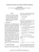
Figure 1: The non-weighted deductive system of top-down dependency parsing algorithm: means “take anything”.
for every arc (x, y) ∈ A
W
and node l in x < l < y
or y < l < x, there is a path x →
∗
l or y →
∗
l.
The proposed algorithm in this paper is for projec-
tive dependency graphs. If a projective dependency
graph is connected, we call it a dependency tree,
and if not, a dependency forest.

3 Top-down Parsing Algorithm
Our proposed algorithm is a transition-based algo-
rithm, which uses stack and queue data structures.
This algorithm formally uses the following state:
ℓ : ⟨i, h, j, S⟩ : π
where ℓ is a step size, S is a stack of trees s
d
| |s
0
where s
0
is a top tree and d is a window size for
feature extraction, i is an index of node on the top
of the input node queue, h is an index of root node
of s
0
, j is an index to indicate the right limit ( j −
1 inclusive) of pred

, and π is a set of pointers to
predictor states, which are states just before putting
the node in h onto stack S. In the deterministic case,
π is a singleton set except for the initial state.
This algorithm has four actions, predict

(pred

),
predict


(pred

), scan and complete(comp). The
deductive system of the top-down algorithm is
shown in Figure 1. The initial state p
0
is a state ini-
tialized by an artificial root node n
0
. This algorithm
applies one action to each state selected from appli-
cable actions in each step. Each of three kinds of
actions, pred, scan, and comp, occurs n times, and
this system takes 3n steps for a complete analysis.
Action pred

puts n
k
onto stack S selected from
the input queue in the range, i ≤ k < h, which is
to the left of the root n
h
in the stack top. Similarly,
action pred

puts a node n
k
onto stack S selected
from the input queue in the range, h < i ≤ k < j,
which is to the right of the root n

h
in the stack top.
The node n
i
on the top of the queue is scanned if it
is equal to the root node n
h
in the stack top. Action
comp creates a directed arc (h
′
, h) from the root h
′
of s
′
0
on a predictor state q to the root h of s
0
on a
current state p if h < i
1
.
The precondition i < h of action pred

means
that the input nodes in i ≤ k < h have not been
predicted yet. Pred

, scan and pred

do not con-

flict with each other since their preconditions i < h,
i = h and h < i do not hold at the same time.
However, this algorithm faces a pred

-comp con-
flict because both actions share the same precondi-
tion h < i, which means that the input nodes in
1 ≤ k ≤ h have been predicted and scanned. This
1
In a single root tree, the special root symbol $
0
has exactly
one child node. Therefore, we do not apply comp action to a
state if its condition satisfies s
1
.h = n
0
∧ ℓ ̸= 3n − 1.
658
step state stack queue action state information
0 p
0
$
0
I
1
saw
2
a
3

girl
4
– ⟨1, 0, 5⟩ : ∅
1 p
1
$
0
|saw
2
I
1
saw
2
a
3
girl
4
pred

⟨1, 2, 5⟩ : {p
0
}
2 p
2
saw
2
|I
1
I
1

saw
2
a
3
girl
4
pred

⟨1, 1, 2⟩ : {p
1
}
3 p
3
saw
2
|I
1
saw
2
a
3
girl
4
scan ⟨2, 1, 2⟩ : {p
1
}
4 p
4
$
0

|I
1

saw
2
saw
2
a
3
girl
4
comp ⟨2, 2, 5⟩ : {p
0
}
5 p
5
$
0
|I
1

saw
2
a
3
girl
4
scan ⟨3, 2, 5⟩ : {p
0
}

6 p
6
I
1

saw
2
|girl
4
a
3
girl
4
pred

⟨3, 4, 5⟩ : {p
5
}
7 p
7
girl
4
|a
3
a
3
girl
4
pred


⟨3, 3, 4⟩ : {p
6
}
8 p
8
girl
4
|a
3
girl
4
scan ⟨4, 3, 4⟩ : {p
6
}
9 p
9
I
1

saw
2
|a
3

girl
4
girl
4
comp ⟨4, 4, 5⟩ : {p
5

}
10 p
10
I
1

saw
2
|a
3

girl
4
scan ⟨5, 4, 5⟩ : {p
5
}
11 p
11
$
0
|I
1

saw
2

girl
4
comp ⟨5, 2, 5⟩ : {p
0

}
12 p
12
$
0

saw
2
comp ⟨5, 0, 5⟩ : ∅
Figure 2: Stages of the top-down deterministic parsing process for a sentence “I saw a girl”. We follow a convention
and write the stack with its topmost element to the right, and the queue with its first element to the left. In this example,
we set the window size d to 1, and write the descendants of trees on stack elements s
0
and s
1
within depth 1.
parser constructs left and right children of a head
node in a left-to-right direction by scanning the head
node prior to its right children. Figure 2 shows an
example for parsing a sentence “I saw a girl”.
4 Correctness
To prove the correctness of the system in Figure
1 for the projective dependency graph, we use the
proof strategy of (Nivre, 2008a). The correct deduc-
tive system is both sound and complete.
Theorem 4.1 The deductive system in Figure 1 is
correct for the class of dependency forest.
Proof 4.1 To show soundness, we show that G
p
0

=
(V
W
, ∅), which is a directed graph defined by the
axiom, is well-formed and projective, and that every
transition preserves this property.
• ROOT: The node 0 is a root in G
p
0
, and the
node 0 is on the top of stack of p
0
. The two pred
actions put a word onto the top of stack, and
predict an arc from root or its descendant to
the child. The comp actions add the predicted
arcs which include no arc of (x, 0).
• SINGLE-HEAD: G
p
0
is single-head. A node
y is no longer in stack and queue after a comp
action creates an arc (x, y). The node y cannot
make any arc
(
x
′
, y
)
after the removal.

• ACYCLICITY: G
p
0
is acyclic. A cycle is cre-
ated only if an arc (x, y) is added when there
is a directed path y →
∗
x. The node x is no
longer in stack and queue when the directed
path y →
∗
x was made by adding an arc (l, x).
There is no chance to add the arc (x, y) on the
directed path y →
∗
x.
• PROJECTIVITY: G
p
0
is projective. Projec-
tivity is violated by adding an arc (x, y) when
there is a node l in x < l < y or y < l < x
with the path to or from the outside of the span
x and y. When pred

creates an arc relation
from x to y, the node y cannot be scanned be-
fore all nodes l in x < l < y are scanned and
completed. When pred


creates an arc rela-
tion from x to y, the node y cannot be scanned
before all nodes k in k < y are scanned and
completed, and the node x cannot be scanned
before all nodes l in y < l < x are scanned
and completed. In those processes, the node l
in x < l < y or y < l < x does not make a
path to or from the outside of the span x and y,
and a path x →
∗
l or y →
∗
l is created. ✷
To show completeness, we show that for any sen-
tence W , and dependency forest G
W
= (V
W
, A
W
),
there is a transition sequence C
0,m
such that G
p
m
=
G
W
by an inductive method.

• If |W | = 1, the projective dependency graph
for W is G
W
= ({0}, ∅) and G
p
0
= G
W
.
• Assume that the claim holds for sentences with
length less or equal to t, and assume that
|W | = t + 1 and G
W
= (V
W
, A
W
). The sub-
graph G
W
′
is defined as (V
W
− t, A
−t
) where
659
.
.
s

2
.h
.
.
.
. .
.
.
.

.
.
s
1
.h
.
.
.
.
.
.
.
.
.

.
.
.
. .
.

s
1
.l
.
.
.
. .
.

.
.
.
. .
.
s
1
.r
.
.
.
. .
.
.
s
0
.h
.
.
.
.

.
.
.
.
.

.
.
.
. .
.
s
0
.l
.
.
.
. .
.

.
.
.
. .
.
s
0
.r
.
.

.
. .
Figure 3: Feature window of trees on stack S: The win-
dow size d is set to 2. Each x.h, x.l and x.r denotes root,
left and right child nodes of a stack element x.
A
−t
= A
W
−{(x, y)|x = t ∨y = t}. If G
W
is
a dependency forest, then G
W
′
is also a depen-
dency forest. It is obvious that there is a transi-
tion sequence for constructing G
W
except arcs
which have a node t as a head or a dependent
2
.
There is a state p
q
= q : ⟨i, x, t + 1⟩ :
for i and x (0 ≤ x < i < t + 1). When
x is the head of t, pred

to t creates a state

p
q+1
= q + 1 : ⟨i, t, t + 1⟩ : {p
q
}. At least one
node y in i ≤ y < t becomes the dependent of
t by pred

and there is a transition sequence
for constructing a tree rooted by y. After con-
structing a subtree rooted by t and spaned from
i to t, t is scaned, and then comp creates an
arc from x to t. It is obvious that the remaining
transition sequence exists. Therefore, we can
construct a transition sequence C
0,m
such that
G
p
m
= G
W
. ✷
The deductive sysmtem in Figure 1 is both sound and
complete. Therefore, it is correct. ✷
5 Weighted Parsing Model
5.1 Stack-based Model
The proposed algorithm employs a stack-based
model for scoring hypothesis. The cost of the model
is defined as follows:

c
s
(i, h, j, S) = θ
s
· f
s,act
(i, h, j, S) (1)
where θ
s
is a weight vector, f
s
is a feature function,
and act is one of the applicable actions to a state ℓ :
⟨i, h, j, S⟩ : π. We use a set of feature templates of
(Huang and Sagae, 2010) for the model. As shown
in Figure 3, left children s
0
.l and s
1
.l of trees on
2
This transition sequence is defined for G
W
′
, but it is pos-
sible to be regarded as the definition for G
W
as long as the
transition sequence is indifferent from the node t.
Algorithm 1 Top-down Parsing with Beam Search

1: input W = n
0
, . . . , n
n
2: start ← ⟨1, 0, n + 1, n
0
⟩
3: buf[0] ← {start}
4: for ℓ ← 1 . . . 3n do
5: hypo ← {}
6: for each state in buf[ℓ −1] do
7: for act ←applicableAct(state) do
8: newstates ←actor(act, state)
9: addAll newstates to hypo
10: add top b states to buf[ℓ] from hypo
11: return best candidate from buf[3n]
stack for extracting features are different from those
of Huang and Sagae (2010) because in our parser the
left children are generated from left to right.
As mentioned in Section 1, we apply beam search
and Huang and Sagae (2010)’s DP techniques to
our top-down parser. Algorithm 1 shows the our
beam search algorithm in which top most b states
are preserved in a buffer buf[ℓ] in each step. In
line 10 of Algorithm 1, equivalent states in the step
ℓ are merged following the idea of DP. Two states
⟨i, h, j, S⟩ and ⟨i
′
, h
′

, j
′
, S
′
⟩ in the step ℓ are equiv-
alent, notated ⟨i, h, j, S⟩ ∼ ⟨i
′
, h
′
, j
′
, S
′
⟩, iff
f
s,act
(i, h, j, S) = f
s,act
(i
′
, h
′
, j
′
, S
′
). (2)
When two equivalent predicted states are merged,
their predictor states in π get combined. For fur-
ther details about this technique, readers may refer

to (Huang and Sagae, 2010).
5.2 Weighted Prediction
The step 0 in Figure 2 shows an example of predic-
tion for a head node “$
0
”, where the node “saw
2
” is
selected as its child node. To select a probable child
node, we define a statistical model for the prediction.
In this paper, we integrate the cost from a graph-
based model (McDonald and Pereira, 2006) which
directly models dependency links. The cost of the
1st-order model is defined as the relation between a
child node c and a head node h:
c
p
(h, c) = θ
p
· f
p
(h, c) (3)
where θ
p
is a weight vector and f
p
is a features func-
tion. Using the cost c
p
, the top-down parser selects

a probable child node in each prediction step.
When we apply beam search to the top-down
parser, then we no longer use ∃ but ∀ on pred

and
660
.
.
h
.
.
.
.
.
.
.
.
.
.
.
.
.
l
1
.
. .
.
l
l
.

r
1
.
. .
.
r
m
Figure 4: An example of tree structure: Each h, l and r
denotes head, left and right child nodes.
pred

in Figure 1. Therefore, the parser may predict
many nodes as an appropriate child from a single
state, causing many predicted states. This may cause
the beam buffer to be filled only with the states, and
these may exclude other states, such as scanned or
completed states. Thus, we limit the number of pre-
dicted states from a single state by prediction size
implicitly in line 10 of Algorithm 1.
To improve the prediction accuracy, we introduce
a more sophisticated model. The cost of the sibling
2nd-order model is defined as the relationship be-
tween c, h and a sibling node sib:
c
p
(h, sib, c) = θ
p
· f
p
(h, sib, c). (4)

The 1st- and sibling 2nd-order models are the same
as McDonald and Pereira (2006)’s definitions, ex-
cept the cost factors of the sibling 2nd-order model.
The cost factors for a tree structure in Figure 4 are
defined as follows:
c
p
(h, −, l
1
) +
l−1
∑
y=1
c
p
(h, l
y
, l
y+1
)
+c
p
(h, −, r
1
) +
m−1
∑
y=1
c
p

(h, r
y
, r
y+1
).
This is different from McDonald and Pereira (2006)
in that the cost factors for left children are calcu-
lated from left to right, while those in McDonald and
Pereira (2006)’s definition are calculated from right
to left. This is because our top-down parser gener-
ates left children from left to right. Note that the
cost of weighted prediction model in this section is
incrementally calculated by using only the informa-
tion on the current state, thus the condition of state
merge in Equation 2 remains unchanged.
5.3 Weighted Deductive System
We extend deductive system to a weighted one, and
introduce forward cost and inside cost (Stolcke,
1995; Huang and Sagae, 2010). The forward cost is
the total cost of a sequence from an initial state to the
end state. The inside cost is the cost of a top tree s
0
in stack S. We define these costs using a combina-
tion of stack-based model and weighted prediction
model. The forward and inside costs of the combi-
nation model are as follows:
{
c
fw
= c

fw
s
+ c
fw
p
c
in
= c
in
s
+ c
in
p
(5)
where c
fw
s
and c
in
s
are a forward cost and an inside
cost for stack-based model, and c
fw
p
and c
in
p
are a for-
ward cost and an inside cost for weighted prediction
model. We add the following tuple of costs to a state:

(c
fw
s
, c
in
s
, c
fw
p
, c
in
p
).
For each action, we define how to efficiently cal-
culate the forward and inside costs
3
, following Stol-
cke (1995) and Huang and Sagae (2010)’s works. In
either case of pred

or pred

,
(c
fw
s
, , c
fw
p
, )

(c
fw
s
+ λ, 0, c
fw
p
+ c
p
(s
0
.h, n
k
), 0)
where
λ =
{
θ
s
· f
s,pred

(i, h, j, S) if pred

θ
s
· f
s,pred

(i, h, j, S) if pred


(6)
In the case of scan,
(c
fw
s
, c
in
s
, c
fw
p
, c
in
p
)
(c
fw
s
+ ξ, c
in
s
+ ξ, c
fw
p
, c
in
p
)
where
ξ = θ

s
· f
s,scan
(i, h, j, S). (7)
In the case of comp,
(c
′
fw
s
, c
′
in
s
, c
′
fw
p
, c
′
in
p
) (c
fw
s
, c
in
s
, c
fw
p

, c
in
p
)
(c
′
fw
s
+ c
in
s
+ µ, c
′
in
s
+ c
in
s
+ µ,
c
′
fw
p
+ c
in
p
+ c
p
(s
′

0
.h, s
0
.h),
c
′
in
p
+ c
in
p
+ c
p
(s
′
0
.h, s
0
.h))
where
µ = θ
s
· f
s,comp
(i, h, j, S) + θ
s
· f
s,pred
( , h
′

, j
′
, S
′
).
(8)
3
For brevity, we present the formula not by 2nd-order model
as equation 4 but a 1st-order one for weighted prediction.
661
Pred takes either pred

or pred

. Beam search is
performed based on the following linear order for
the two states p and p
′
at the same step, which have
(c
fw
, c
in
) and (c
′
fw
, c
′
in
) respectively:

p ≻ p
′
iff c
fw
< c
′
fw
or c
fw
= c
′
fw
∧ c
in
< c
′
in
. (9)
We prioritize the forward cost over the inside cost
since forward cost pertains to longer action sequence
and is better suited to evaluate hypothesis states than
inside cost (Nederhof, 2003).
5.4 FIRST Function for Lookahead
Top-down backtrack parser usually reduces back-
tracking by precomputing the set FIRST(·) (Aho and
Ullman, 1972). We define the set FIRST(·) for our
top-down dependency parser:
FIRST(t’) = {ld.t|ld ∈ lmdescendant(Tree, t’)
Tree ∈ Corpus}(10)
where t’ is a POS-tag, Tree is a correct depen-

dency tree which exists in Corpus, a function
lmdescendant(Tree, t’) returns the set of the leftmost
descendant node ld of each nodes in Tree whose
POS-tag is t’, and ld.t denotes a POS-tag of ld.
Though our parser does not backtrack, it looks ahead
when selecting possible child nodes at the prediction
step by using the function FIRST. In case of pred

:
∀k : i ≤ k < h ∧ n
i
.t ∈ FIRST(n
k
.t)
state p
  
ℓ : ⟨i, h, j, s
d
| |s
0
⟩ :
ℓ + 1 : ⟨i, k, h, s
d−1
| |s
0
|n
k
⟩ : {p}
where n
i

.t is a POS-tag of the node n
i
on the top of
the queue, and n
k
.t is a POS-tag in kth position of
an input nodes. The case for pred

is the same. If
there are no nodes which satisfy the condition, our
top-down parser creates new states for all nodes, and
pushes them into hypo in line 9 of Algorithm 1.
6 Time Complexity
Our proposed top-down algorithm has three kinds
of actions which are scan, comp and predict. Each
scan and comp actions occurs n times when parsing
a sentence with the length n. Predict action also oc-
curs n times in which a child node is selected from
a node sequence in the input queue. Thus, the algo-
rithm takes the following times for prediction:
n + (n −1) + ··· + 1 =
n
∑
i
i =
n(n + 1)
2
. (11)
As n
2

for prediction is the most dominant factor, the
time complexity of the algorithm is O(n
2
) and that
of the algorithm with beam search is O(n
2
∗ b).
7 Related Work
Alshawi (1996) proposed head automaton which
recognizes an input sentence top-down. Eisner
and Satta (1999) showed that there is a cubic-time
parsing algorithm on the formalism of the head
automaton grammars, which are equivalently con-
verted into split-head bilexical context-free gram-
mars (SBCFGs) (McAllester, 1999; Johnson, 2007).
Although our proposed algorithm does not employ
the formalism of SBCFGs, it creates left children
before right children, implying that it does not have
spurious ambiguities as well as parsing algorithms
on the SBCFGs. Head-corner parsing algorithm
(Kay, 1989) creates dependency tree top-down, and
in this our algorithm has similar spirit to it.
Yamada and Matsumoto (2003) applied a shift-
reduce algorithm to dependency analysis, which is
known as arc-standard transition-based algorithm
(Nivre, 2004). Nivre (2003) proposed another
transition-based algorithm, known as arc-eager al-
gorithm. The arc-eager algorithm processes right-
dependent top-down, but this does not involve the
prediction of lower nodes from higher nodes. There-

fore, the arc-eager algorithm is a totally bottom-up
algorithm. Zhang and Clark (2008) proposed a com-
bination approach of the transition-based algorithm
with graph-based algorithm (McDonald and Pereira,
2006), which is the same as our combination model
of stack-based and prediction models.
8 Experiments
Experiments were performed on the English Penn
Treebank data and the Chinese CoNLL-06 data. For
the English data, we split WSJ part of it into sections
02-21 for training, section 22 for development and
section 23 for testing. We used Yamada and Mat-
sumoto (2003)’s head rules to convert phrase struc-
ture to dependency structure. For the Chinese data,
662
time accuracy complete root
McDonald05,06 (2nd) 0.15 90.9, 91.5 37.5, 42.1 –
Koo10 (Koo and Collins, 2010) – 93.04 – –
Hayashi11 (Hayashi et al., 2011) 0.3 92.89 – –
2nd-MST
∗
0.13 92.3 43.7 96.0
Goldberg10 (Goldberg and Elhadad, 2010) – 89.7 37.5 91.5
Kitagawa10 (Kitagawa and Tanaka-Ishii, 2010) – 91.3 41.7 –
Zhang08 (Sh beam 64) – 91.4 41.8 –
Zhang08 (Sh+Graph beam 64) – 92.1 45.4 –
Huang10 (beam+DP) 0.04 92.1 – –
Huang10
∗
(beam 8, 16, 32+DP) 0.03, 0.06, 0.10 92.3, 92.27, 92.26 43.5, 43.7, 43.8 96.0, 96.0, 96.1

Zhang11 (beam 64) (Zhang and Nivre, 2011) – 93.07 49.59 –
top-down
∗
(beam 8, 16, 32+pred 5+DP) 0.07, 0.12, 0.22 91.7, 92.3, 92.5 45.0, 45.7, 45.9 94.5, 95.7, 96.2
top-down
∗
(beam 8, 16, 32+pred 5+DP+FIRST) 0.07, 0.12, 0.22 91.9, 92.4, 92.6 45.0, 45.3, 45.5 95.1, 96.2, 96.6
Table 1: Results for test data: Time measures the parsing time per sentence in seconds. Accuracy is an unlabeled
attachment score, complete is a sentence complete rate, and root is a correct root rate. ∗ indicates our experiments.
0
0.2
0.4
0.6
0.8
1
0 10 20 30 40 50 60 70
parsing time (cpu sec)
length of input sentence
"shift-reduce"
"2nd-mst"
"top-down"
Figure 5: Scatter plot of parsing time against sentence
length, comparing with top-down, 2nd-MST and shift-
reduce parsers (beam size: 8, pred size: 5)
we used the information of words and fine-grained
POS-tags for features. We also implemented and ex-
perimented Huang and Sagae (2010)’s arc-standard
shift-reduce parser. For the 2nd-order Eisner-Satta
algorithm, we used MSTParser (McDonald, 2012).
We used an early update version of averaged per-

ceptron algorithm (Collins and Roark, 2004) for
training of shift-reduce and top-down parsers. A
set of feature templates in (Huang and Sagae, 2010)
were used for the stack-based model, and a set of
feature templates in (McDonald and Pereira, 2006)
were used for the 2nd-order prediction model. The
weighted prediction and stack-based models of top-
down parser were jointly trained.
8.1 Results for English Data
During training, we fixed the prediction size and
beam size to 5 and 16, respectively, judged by pre-
accuracy complete root
oracle (sh+mst) 94.3 52.3 97.7
oracle (top+sh) 94.2 51.7 97.6
oracle (top+mst) 93.8 50.7 97.1
oracle (top+sh+mst) 94.9 55.3 98.1
Table 2: Oracle score, choosing the highest accuracy
parse for each sentence on test data from results of top-
down (beam 8, pred 5) and shift-reduce (beam 8) and
MST(2nd) parsers in Table 1.
accuracy complete root
top-down (beam:8, pred:5) 90.9 80.4 93.0
shift-reduce (beam:8) 90.8 77.6 93.5
2nd-MST 91.4 79.3 94.2
oracle (sh+mst) 94.0 85.1 95.9
oracle (top+sh) 93.8 84.0 95.6
oracle (top+mst) 93.6 84.2 95.3
oracle (top+sh+mst) 94.7 86.5 96.3
Table 3: Results for Chinese Data (CoNLL-06)
liminary experiments on development data. After

25 iterations of perceptron training, we achieved
92.94 unlabeled accuracy for top-down parser with
the FIRST function and 93.01 unlabeled accuracy
for shift-reduce parser on development data by set-
ting the beam size to 8 for both parsers and the pre-
diction size to 5 in top-down parser. These trained
models were used for the following testing.
We compared top-down parsing algorithm with
other data-driven parsing algorithms in Table 1.
Top-down parser achieved comparable unlabeled ac-
curacy with others, and outperformed them on the
sentence complete rate. On the other hand, top-
down parser was less accurate than shift-reduce
663
No.717 Little Lily , as Ms. Cunningham calls
7
herself in the book , really was
14
n’t ordinary .
shift-reduce 2 7 2 2 6 4 14 7 7 11 9 7 14 0 14 14 14
2nd-MST 2 14 2 2 6 7 4 7 7 11 9 2 14 0 14 14 14
top-down 2 14 2 2 6 7 4 7 7 11 9 2 14 0 14 14 14
correct 2 14 2 2 6 7 4 7 7 11 9 2 14 0 14 14 14
No.127 resin , used to make garbage bags , milk jugs , housewares , toys and meat packaging
25
, among other items .
shift-reduce 25 9 9 13 11 15 13 25 18 25 25 25 25 25 25 25 7 25 25 29 27 4
2nd-MST 29 9 9 13 11 15 13 29 18 29 29 29 29 25 25 25 29 25 25 29 7 4
top-down 7 9 9 13 11 15 25 25 18 25 25 25 25 25 25 25 13 25 25 29 27 4
correct 7 9 9 13 11 15 25 25 18 25 25 25 25 25 25 25 13 25 25 29 27 4

Table 4: Two examples on which top-down parser is superior to two bottom-up parsers: In correct analysis, the boxed
portion is the head of the underlined portion. Bottom-up parsers often mistake to capture the relation.
parser on the correct root measure. In step 0, top-
down parser predicts a child node, a root node of
a complete tree, using little syntactic information,
which may lead to errors in the root node selection.
Therefore, we think that it is important to seek more
suitable features for the prediction in future work.
Figure 5 presents the parsing time against sen-
tence length. Our proposed top-down parser is the-
oretically slower than shift-reduce parser and Fig-
ure 5 empirically indicates the trends. The domi-
nant factor comes from the score calculation, and
we will leave it for future work. Table 2 shows
the oracle score for test data, which is the score
of the highest accuracy parse selected for each sen-
tence from results of several parsers. This indicates
that the parses produced by each parser are differ-
ent from each other. However, the gains obtained by
the combination of top-down and 2nd-MST parsers
are smaller than other combinations. This is because
top-down parser uses the same features as 2nd-MST
parser, and these are more effective than those of
stack-based model. It is worth noting that as shown
in Figure 5, our O(n
2
∗b) (b = 8) top-down parser is
much faster than O(n
3
) Eisner-Satta CKY parsing.

8.2 Results for Chinese Data (CoNLL-06)
We also experimented on the Chinese data. Fol-
lowing English experiments, shift-reduce parser was
trained by setting beam size to 16, and top-down
parser was trained with the beam size and the predic-
tion size to 16 and 5, respectively. Table 3 shows the
results on the Chinese test data when setting beam
size to 8 for both parsers and prediction size to 5 in
top-down parser. The trends of the results are almost
the same as those of the English results.
8.3 Analysis of Results
Table 4 shows two interesting results, on which top-
down parser is superior to either shift-reduce parser
or 2nd-MST parser. The sentence No.717 contains
an adverbial clause structure between the subject
and the main verb. Top-down parser is able to han-
dle the long-distance dependency while shift-reudce
parser cannot correctly analyze it. The effectiveness
on the clause structures implies that our head-driven
parser may handle non-projective structures well,
which are introduced by Johansonn’s head rule (Jo-
hansson and Nugues, 2007). The sentence No.127
contains a coordination structure, which it is diffi-
cult for bottom-up parsers to handle, but, top-down
parser handles it well because its top-down predic-
tion globally captures the coordination.
9 Conclusion
This paper presents a novel head-driven parsing al-
gorithm and empirically shows that it is as practi-
cal as other dependency parsing algorithms. Our

head-driven parser has potential for handling non-
projective structures better than other non-projective
dependency algorithms (McDonald et al., 2005; At-
tardi, 2006; Nivre, 2008b; Koo et al., 2010). We are
in the process of extending our head-driven parser
for non-projective structures as our future work.
Acknowledgments
We would like to thank Kevin Duh for his helpful
comments and to the anonymous reviewers for giv-
ing valuable comments.
664
References
A. V. Aho and J. D. Ullman. 1972. The Theory of Pars-
ing, Translation and Compiling, volume 1: Parsing.
Prentice-Hall.
H. Alshawi. 1996. Head automata for speech translation.
In Proc. the ICSLP.
G. Attardi. 2006. Experiments with a multilanguage
non-projective dependency parser. In Proc. the 10th
CoNLL, pages 166–170.
M. Collins and B. Roark. 2004. Incremental parsing with
the perceptron algorithm. In Proc. the 42nd ACL.
J. Earley. 1970. An efficient context-free parsing algo-
rithm. Communications of the Association for Com-
puting Machinery, 13(2):94–102.
J. M. Eisner and G. Satta. 1999. Efficient parsing for
bilexical context-free grammars and head automaton
grammars. In Proc. the 37th ACL, pages 457–464.
Y. Goldberg and M. Elhadad. 2010. An efficient algo-
rithm for easy-first non-directional dependency pars-

ing. In Proc. the HLT-NAACL, pages 742–750.
K. Hayashi, T. Watanabe, M. Asahara, and Y. Mat-
sumoto. 2011. The third-order variational rerank-
ing on packed-shared dependency forests. In Proc.
EMNLP, pages 1479–1488.
L. Huang and K. Sagae. 2010. Dynamic programming
for linear-time incremental parsing. In Proc. the 48th
ACL, pages 1077–1086.
H. Isozaki, H. Kazawa, and T. Hirao. 2004. A determin-
istic word dependency analyzer enhanced with prefer-
ence learning. In Proc. the 21st COLING, pages 275–
281.
R. Johansson and P. Nugues. 2007. Extended
constituent-to-dependency conversion for english. In
Proc. NODALIDA.
M. Johnson. 2007. Transforming projective bilexical
dependency grammars into efficiently-parsable CFGs
with unfold-fold. In Proc. the 45th ACL, pages 168–
175.
M. Kay. 1989. Head driven parsing. In Proc. the IWPT.
K. Kitagawa and K. Tanaka-Ishii. 2010. Tree-based de-
terministic dependency parsing — an application to
nivre’s method —. In Proc. the 48th ACL 2010 Short
Papers, pages 189–193, July.
T. Koo and M. Collins. 2010. Efficient third-order de-
pendency parsers. In Proc. the 48th ACL, pages 1–11.
T. Koo, A. M. Rush, M. Collins, T. Jaakkola, and D. Son-
tag. 2010. Dual decomposition for parsing with non-
projective head automata. In Proc. EMNLP, pages
1288–1298.

D. McAllester. 1999. A reformulation of eisner and
satta’s cubic time parser for split head automata gram-
mars. dmcallester/.
R. McDonald and F. Pereira. 2006. Online learning of
approximate dependency parsing algorithms. In Proc.
EACL, pages 81–88.
R. McDonald, F. Pereira, K. Ribarov, and J. Hajic. 2005.
Non-projective dependency parsing using spanning
tree algorithms. In Proc. HLT-EMNLP, pages 523–
530.
R. McDonald. 2012. Minimum spanning tree parser.
strctlrn/MSTParser.
M J. Nederhof. 2003. Weighted deductive parsing
and knuth’s algorithm. Computational Linguistics,
29:135–143.
J. Nivre. 2003. An efficient algorithm for projective de-
pendency parsing. In Proc. the IWPT, pages 149–160.
J. Nivre. 2004. Incrementality in deterministic depen-
dency parsing. In Proc. the ACL Workshop Incremen-
tal Parsing: Bringing Engineering and Cognition To-
gether, pages 50–57.
J. Nivre. 2006. Inductive Dependency Parsing. Springer.
J. Nivre. 2008a. Algorithms for deterministic incremen-
tal dependency parsing. Computational Linguistics,
34:513–553.
J. Nivre. 2008b. Sorting out dependency parsing. In
Proc. the CoTAL, pages 16–27.
A. Stolcke. 1995. An efficient probabilistic context-free
parsing algorithm that computes prefix probabilities.
Computational Linguistics, 21(2):165–201.

H. Yamada and Y. Matsumoto. 2003. Statistical depen-
dency analysis with support vector machines. In Proc.
the IWPT, pages 195–206.
Y. Zhang and S. Clark. 2008. A tale of two parsers: In-
vestigating and combining graph-based and transition-
based dependency parsing using beam-search. In
Proc. EMNLP, pages 562–571.
Y. Zhang and J. Nivre. 2011. Transition-based depen-
dency parsing with rich non-local features. In Proc.
the 49th ACL, pages 188–193.
665