Báo cáo khoa học: "Optimal rank reduction for Linear Context-Free Rewriting Systems with Fan-Out Two" pot
Bạn đang xem bản rút gọn của tài liệu. Xem và tải ngay bản đầy đủ của tài liệu tại đây (233.2 KB, 9 trang )
Proceedings of the 48th Annual Meeting of the Association for Computational Linguistics, pages 525–533,
Uppsala, Sweden, 11-16 July 2010.
c
2010 Association for Computational Linguistics
Optimal rank reduction
for Linear Context-Free Rewriting Systems with Fan-Out Two
Benot Sagot
INRIA & Universit´e Paris 7
Le Chesnay, France
Giorgio Satta
Department of Information Engineering
University of Padua, Italy
Abstract
Linear Context-Free Rewriting Systems
(LCFRSs) are a grammar formalism ca-
pable of modeling discontinuous phrases.
Many parsing applications use LCFRSs
where the fan-out (a measure of the dis-
continuity of phrases) does not exceed 2.
We present an efficient algorithm for opti-
mal reduction of the length of production
right-hand side in LCFRSs with fan-out at
most 2. This results in asymptotical run-
ning time improvement for known parsing
algorithms for this class.
1 Introduction
Linear Context-Free Rewriting Systems
(LCFRSs) have been introduced by Vijay-
Shanker et al. (1987) for modeling the syntax
of natural language. The formalism extends the
generative capacity of context-free grammars, still
remaining far below the class of context-sensitive
grammars. An important feature of LCFRSs is
their ability to generate discontinuous phrases.
This has been recently exploited for modeling
phrase structure treebanks with discontinuous
constituents (Maier and Søgaard, 2008), as well as
non-projective dependency treebanks (Kuhlmann
and Satta, 2009).
The maximum number f of tuple components
that can be generated by an LCFRS G is called
the fan-out of G, and the maximum number r of
nonterminals in the right-hand side of a production
is called the rank of G. As an example, context-
free grammars are LCFRSs with f = 1 and r
given by the maximum length of a production
right-hand side. Tree adjoining grammars (Joshi
and Levy, 1977) can also be viewed as a special
kind of LCFRS with f = 2, since each auxil-
iary tree generates two strings, and with r given
by the maximum number of adjunction and sub-
stitution sites in an elementary tree. Beyond tree
adjoining languages, LCFRSs with f = 2 can
also generate languages in which pair of strings
derived from different nonterminals appear in so-
called crossing configurations. It has recently been
observed that, in this way, LCFRSs with f = 2
can model the vast majority of data in discontinu-
ous phrase structure treebanks and non-projective
dependency treebanks (Maier and Lichte, 2009;
Kuhlmann and Satta, 2009).
Under a theoretical perspective, the parsing
problem for LCFRSs with f = 2 is NP-complete
(Satta, 1992), and in known parsing algorithms
the running time is exponentially affected by the
rank r of the grammar. Nonetheless, in natu-
ral language parsing applications, it is possible to
achieve efficient, polynomial parsing if we suc-
ceed in reducing the rank r (number of nontermi-
nals in the right-hand side) of individual LCFRSs’
productions (Kuhlmann and Satta, 2009). This
process is called production factorization. Pro-
duction factorization is very similar to the reduc-
tion of a context-free grammar production into
Chomsky normal form. However, in the LCFRS
case some productions might not be reducible to
r = 2, and the process stops at some larger value
for r, which in the worst case might as well be the
rank of the source production (Rambow and Satta,
1999).
Motivated by parsing efficiency, the factoriza-
tion problem for LCFRSs with f = 2 has at-
tracted the attention of many researchers in recent
years. Most of the literature has been focusing on
binarization algorithms, which attempt to find a re-
duction to r = 2 and return a failure if this is not
possible. G´omez-Rodr´ıguez et al. (2009) report a
general binarization algorithm for LCFRS which,
in the case of f = 2, works in time O(|p|
7
), where
|p| is the size of the input production. A more ef-
ficient binarization algorithm for the case f = 2 is
presented in (G´omez-Rodr´ıguez and Satta, 2009),
working in time O(|p|).
525
In this paper we are interested in general factor-
ization algorithms, i.e., algorithms that find factor-
izations with the smallest possible rank (not nec-
essarily r = 2). We present a novel technique that
solves the general factorization problem in time
O(|p|
2
) for LCFRSs with f = 2.
Strong generative equivalence results between
LCFRS and other finite copying parallel rewrit-
ing systems have been discussed in (Weir, 1992)
and in (Rambow and Satta, 1999). Through these
equivalence results, we can transfer the factoriza-
tion techniques presented in this article to other
finite copying parallel rewriting systems.
2 LCFRSs
In this section we introduce the basic notation for
LCFRS and the notion of production factoriza-
tion.
2.1 Definitions
Let Σ
T
be a finite alphabet of terminal symbols.
As usual, Σ
∗
T
denotes the set of all finite strings
over Σ
T
, including the empty string ε. For in-
teger k ≥ 1, (Σ
∗
T
)
k
denotes the set of all tuples
(w
1
, . . . , w
k
) of strings w
i
∈ Σ
∗
T
. In what follows
we are interested in functions mapping several tu-
ples of strings in Σ
∗
T
into tuples of strings in Σ
∗
T
.
Let r and f be two integers, r ≥ 0 and f ≥ 1.
We say that a function g has rank r if there exist
integers f
i
≥ 1, 1 ≤ i ≤ r, such that g is defined
on (Σ
∗
T
)
f
1
× (Σ
∗
T
)
f
2
× · ·· × (Σ
∗
T
)
f
r
. We also say
that g has fan-out f if the range of g is a subset of
(Σ
∗
T
)
f
. Let y
h
, x
ij
, 1 ≤ h ≤ f, 1 ≤ i ≤ r and
1 ≤ j ≤ f
i
, be string-valued variables. A func-
tion g as above is said to be linear regular if it is
defined by an equation of the form
g(x
11
, . . . , x
1f
1
, . . . , x
r1
, . . . , x
rf
r
) =
= y
1
, . . . , y
f
, (1)
where y
1
, . . . , y
f
represents some grouping into
f sequences of all and only the variables appear-
ing in the left-hand side of (1) (without repeti-
tions) along with some additional terminal sym-
bols (with possible repetitions).
For a mathematical definition of LCFRS we re-
fer the reader to (Weir, 1992, p. 137). Informally,
in a LCFRS every nonterminal symbol A is asso-
ciated with an integer ϕ(A) ≥ 1, called its fan-out,
and it generates tuples in (Σ
∗
T
)
ϕ(A)
. Productions
in a LCFRS have the form
p : A → g(B
1
, B
2
, . . . , B
ρ(p)
),
where ρ(p) ≥ 0, A and B
i
, 1 ≤ i ≤ ρ(p), are non-
terminal symbols, and g is a linear regular func-
tion having rank ρ(p) and fan-out ϕ(A), defined
on (Σ
∗
T
)
ϕ(B
1
)
× · · · × (Σ
∗
T
)
ϕ(B
ρ(p)
)
and taking val-
ues in (Σ
∗
T
)
ϕ(A)
. The basic idea underlying the
rewriting relation associated with LCFRS is that
production p applies to any sequence of string tu-
ples generated by the B
i
’s, and provides a new
string tuple in (Σ
∗
T
)
ϕ(A)
obtained through function
g. We say that ϕ(p) = ϕ(A) is the fan-out of p,
and ρ(p) is the rank of p.
Example 1 Let L be the language L =
{a
n
b
n
a
m
b
m
a
n
b
n
a
m
b
m
| n, m ≥ 1}. A LCFRS
generating L is defined by means of the nonter-
minals S, ϕ(S) = 1, and A, ϕ(A) = 2, and the
productions in figure 1. Observe that nonterminal
A generates all tuples of the form a
n
b
n
, a
n
b
n
.
✷
Recognition and parsing for a given LCFRS
can be carried out in polynomial time on the length
of the input string. This is usually done by exploit-
ing standard dynamic programming techniques;
see for instance (Seki et al., 1991).
1
However, the
polynomial degree in the running time is a mono-
tonically strictly increasing function that depends
on both the rank and the fan-out of the productions
in the grammar. To optimize running time, one can
then recast the source grammar in such a way that
the value of the above function is kept to a min-
imum. One way to achieve this is by factorizing
the productions of a LCFRS, as we now explain.
2.2 Factorization
Consider a LCFRS production of the form
p : A → g(B
1
, B
2
, . . . , B
ρ(p)
), where g is
specified as in (1). Let also C be a subset of
{B
1
, B
2
, . . . , B
ρ(p)
} such that |C| = 0 and |C| =
ρ(p). We let Σ
C
be the alphabet of all variables
x
ij
defined as in (1), for all values of i and j such
that B
i
∈ C and 1 ≤ j ≤ f
i
. For each i with
1 ≤ i ≤ f, we rewrite each string y
i
in (1) in a
form y
i
= y
′
i0
z
i1
y
′
i1
· · · y
′
id
i−1
z
id
i
y
′
id
i
, with d
i
≥ 0,
such that the following conditions are all met:
• each z
ij
, 1 ≤ j ≤ d
i
, is a string with one or
more occurrences of variables, all in Σ
C
;
• each y
′
ij
, 1 ≤ j ≤ d
i
− 1, is a non-empty
string with no occurrences of symbols in Σ
C
;
• y
′
0j
and y
′
0d
i
are (possibly empty) strings with
no occurrences of symbols in Σ
C
.
1
In (Seki et al., 1991) a syntactic variant of LCFRS is
used, called multiple context-free grammars.
526
S → g
S
(A, A), g
S
(x
11
, x
12
, x
21
, x
22
) = x
11
x
21
x
12
x
22
;
A → g
A
(A), g
A
(x
11
, x
12
) = ax
11
b, ax
12
b;
A → g
′
A
(), g
′
A
() = ab, ab.
Figure 1: A LCFRS for language L = {a
n
b
n
a
m
b
m
a
n
b
n
a
m
b
m
| n, m ≥ 1}.
Let c = |C| and
c = ρ(p) − |C|. Assume that
C = {B
h
1
, . . . , B
h
c
}, and {B
1
, . . . , B
ρ(p)
} − C =
{B
h
′
1
, . . . , B
h
′
c
}. We introduce a fresh nontermi-
nal C with ϕ(C) =
f
i=1
d
i
and replace pro-
duction p in our grammar by means of the two
new productions p
1
: C → g
1
(B
h
1
, . . . , B
h
c
) and
p
2
: A → g
2
(C, B
h
′
1
, . . . , B
h
′
c
). Functions g
1
and
g
2
are defined as:
g
1
(x
h
1
1
, . . . , x
h
1
f
h
1
, . . . , x
h
c
1
, . . . , x
h
c
f
h
c
)
= z
11
, · · · , z
1d
1
, z
21
, · · · , z
fd
f
;
g
2
(x
h
′
1
1
, . . . , x
h
′
1
f
h
′
1
, . . . , x
h
′
c
1
, . . . , x
h
′
c
f
h
′
c
)
= y
′
10
, . . . , y
′
1d
1
, y
′
20
, . . . , y
′
fd
f
.
Note that productions p
1
and p
2
have rank strictly
smaller than the source production p. Further-
more, if it is possible to choose set C in such a
way that
f
i=0
d
i
≤ f , then the fan-out of p
1
and
p
2
will be no greater than the fan-out of p.
We can iterate the procedure above as many
times as possible, under the condition that the fan-
out of the productions does not increase.
Example 2 Let us consider the following produc-
tion with rank 4:
A → g
S
(B, C, D, E),
g
A
(x
11
, x
12
, x
21
, x
22
, x
31
, x
32
, x
41
, x
42
)
= x
11
x
21
x
31
x
41
x
12
x
42
, x
22
x
32
.
Applyng the above procedure twice, we obtain a
factorization consisting of three productions with
rank 2 (variables have been renamed to reflect our
conventions):
A → g
A
(A
1
, A
2
),
g
A
(x
11
, x
12
, x
21
, x
22
)
= x
11
x
21
x
12
, x
22
;
A
1
→ g
A
1
(B, E),
g
A
1
(x
11
, x
12
, x
21
, x
22
) = x
11
, x
21
x
12
x
22
;
A
2
→ g
A
2
(C, D),
g
A
2
(x
11
, x
12
, x
21
, x
22
) = x
11
x
21
, x
12
x
22
.
✷
The factorization procedure above should be ap-
plied to all productions of a LCFRS with rank
larger than two. This might result in an asymptotic
improvement of the running time of existing dy-
namic programming algorithms for parsing based
on LCFRS.
The factorization technique we have discussed
can also be viewed as a generalization of well-
known techniques for casting context-free gram-
mars into binary forms. These are forms where no
more than two nonterminal symbols are found in
the right-hand side of productions of the grammar;
see for instance (Harrison, 1978). One important
difference is that, while production factorization
into binary form is always possible in the context-
free case, for LCFRS there are worst case gram-
mars in which rank reduction is not possible at all,
as shown in (Rambow and Satta, 1999).
3 A graph-based representation for
LCFRS productions
Rather than factorizing LCFRS productions di-
rectly, in this article we work with a more abstract
representation of productions based on graphs.
From now on we focus on LCFRS whose non-
terminals and productions all have fan-out smaller
than or equal to 2. Consider then a production p :
A → g(B
1
, B
2
, . . . , B
ρ(p)
), with ϕ(A), ϕ(B
i
) ≤
2, 1 ≤ i ≤ ρ(p), and with g defined as
g(x
11
, . . . , x
1ϕ(B
1
)
, . . .
. . . , x
ρ(p)1
, . . . , x
ρ(p)ϕ(B
ρ(p)
)
)
= y
1
, . . . , y
ϕ(A)
.
In what follows, if ϕ(A) = 1 then y
1
, . . . , y
ϕ(A)
should be read as y
1
and y
1
· · · y
ϕ(A)
should be
read as y
1
. The same convention applies to all
other nonterminals and tuples.
We now introduce a special kind of undirected
graph that is associated with a linear order defined
over the set of its vertices. The p-graph associated
with production p is a triple (V
p
, E
p
, ≺
p
) such that
• V
p
= {x
ij
| 1 ≤ i ≤ ρ(p), ϕ(B
i
) = 2, 1 ≤
j ≤ ϕ(B
i
)} is a set of vertices;
2
2
Here we are overloading symbols x
ij
. It will always be
clear from the context whether x
ij
is a string-valued variable
or a vertex in a p-graph.
527
• E
p
= {(x
i1
, x
i2
) | x
i1
, x
i2
∈ V
p
} is a set of
undirected edges;
• for x, x
′
∈ V
p
, x ≺
p
x
′
if x = x
′
and the
(unique) occurrence of x in y
1
· · · y
ϕ(A)
pre-
cedes the (unique) occurrence of x
′
.
Note that in the above definition we are ignor-
ing all string-valued variables x
ij
associated with
nonterminals B
i
with ϕ(B
i
) = 1. This is be-
cause nonterminals with fan-out one can always
be treated as in the context-free grammar case, as
it will be explained later.
Example 3 The p-graph associated with the
LCFRS production in Example 2 is shown in Fig-
ure 2. Circled sets of edges indicate the factoriza-
tion in that example.
✷
x
21
x
31
x
41
x
11
B
C
D
E
A
1
A
2
x
42
x
12
x
22
x
32
Figure 2: The p-graph associated with the LCFRS
production in Example 2.
We close this section by introducing some ad-
ditional notation related to p-graphs that will be
used throughout this paper. Let E ⊆ E
p
be some
set of edges. The cover set for E is defined as
V (E) = {x | (x, x
′
) ∈ E} (recall that our edges
are unordered pairs, so (x, x
′
) and (x
′
, x) denote
the same edge). Conversely, let V ⊆ V
p
be some
set of vertices. The incident set for V is defined
as E(V ) = {(x, x
′
) | (x, x
′
) ∈ E
p
, x ∈ V }.
Assume ϕ(p) = 2, and let x
1
, x
2
∈ V
p
. If x
1
and x
2
do not occur both in the same string y
1
or
y
2
, then we say that there is a gap between x
1
and
x
2
. If x
1
≺
p
x
2
and there is no gap between x
1
and x
2
, then we write [x
1
, x
2
] to denote the set
{x
1
, x
2
} ∪ {x | x ∈ V
p
, x
1
≺
p
x ≺
p
x
2
}. For x ∈
V
p
we also let [x, x] = {x}. A set [x, x
′
] is called a
range. Let r and r
′
be two ranges. The pair (r, r
′
)
is called a tandem if the following conditions are
both satisfied: (i) r∪r
′
is not a range, and (ii) there
exists some edge (x, x
′
) ∈ E
p
with x ∈ r and
x
′
∈ r
′
. Note that the first condition means that r
and r
′
are disjoint sets and, for any pair of vertices
x ∈ r and x
′
∈ r
′
, either there is a gap between x
and x
′
or else there exists some x
g
∈ V
p
such that
x ≺
p
x
g
≺
p
x
′
and x
g
∈ r ∪ r
′
.
A set of edges E ⊆ E
p
is called a bundle with
fan-out one if V (E) = [x
1
, x
2
] for some x
1
, x
2
∈
V
p
, i.e., V (E) is a range. Set E is called a bundle
with fan-out two if V (E) = [x
1
, x
2
] ∪ [x
3
, x
4
] for
some x
1
, x
2
, x
3
, x
4
∈ V
p
, and ([x
1
, x
2
], [x
3
, x
4
])
is a tandem. Note that if E is a bundle with fan-out
two with V (E) = [x
1
, x
2
] ∪ [x
3
, x
4
], then neither
E([x
1
, x
2
]) nor E([x
3
, x
4
]) are bundles with fan-
out one, since there is at least one edge incident
upon a vertex in [x
1
, x
2
] and a vertex in [x
3
, x
4
].
We also use the term bundle to denote a bundle
with fan-out either one or two.
Intuitively, in a p-graph associated with a
LCFRS production p, a bundle E with fan-out f
and with |E| > 1 identifies a set of nonterminals
C in the right-hand side of p that can be factorized
into a new production. The nonterminals in C are
then replaced in p by a fresh nonterminal C with
fan-out f , as already explained. Our factorization
algorithm is based on efficient methods for the de-
tection of bundles with fan-out one and two.
4 The algorithm
In this section we provide an efficient, recursive
algorithm for the decomposition of a p-graph into
bundles, which corresponds to factorizing the rep-
resented LCFRS production.
4.1 Overview of the algorithm
The basic idea underlying our graph-based algo-
rithm can be described as follows. We want to
compute an optimal hierarchical decomposition of
an input bundle with fan-out 1 or 2. This decom-
position can be represented by a tree, in which
each node N corresponds to a bundle (the root
node corresponds to the input bundle) and the
daughters of N represent the bundles in which N
is immediately decomposed. The decomposition
is optimal in so far as the maximum arity of the
decomposition tree is as small as possible. As
already explained above, this decomposition rep-
resents a factorization of some production p of a
LCFRS, resulting in optimal rank reduction. All
the internal nodes in the decomposition represent
fresh nonterminals that will be created during the
factorization process.
The construction of the decomposition tree is
carried out recursively. For a given bundle with
fan-out 1 or 2, we apply a procedure for decom-
posing this bundle in its immediate sub-bundles
with fan-out 1 or 2, in an optimal way. Then,
528
we recursively apply our procedure to the obtained
sub-bundles. Recursion stops when we reach bun-
dles containing only one edge (which correspond
to the nonterminals in the right-hand side of the
input production). We shall prove that the result is
an optimal decomposition.
The procedure for computing an optimal de-
composition of a bundle F into its immediate sub-
bundles, which we describe in the first part of this
section, can be sketched as follows. First, we iden-
tify and temporarily remove all maximal bundles
with fan-out 1 (Section 4.3). The result is a new
bundle F
′
which is a subset of the original bundle,
and has the same fan-out. Next, we identify all
sub-bundles with fan-out 2 in F
′
(Section 4.4). We
compute the optimal decomposition of F
′
, rest-
ing on the hypothesis that there are no sub-bundles
with fan-out 1. Each resulting sub-bundle is later
expanded with the maximal sub-bundles with fan-
out 1 that have been previously removed. This re-
sults in a “first level” decomposition of the original
bundle F . We then recursively decompose all in-
dividual sub-bundles of F , including the bundles
with fan-out 1 that have been later attached.
4.2 Backward and forward quantities
For a set V ⊆ V
p
of vertices, we write max(V )
(resp. min(V )) the maximum (resp. minimum)
vertex in V w.r.t. the ≺
p
total order.
Let r = [x
1
, x
2
] be a range. We write r.left =
x
1
and r.right = x
2
. The set of backward edges
for r is defined as B
r
= {(x, x
′
) | (x, x
′
) ∈
E
r
, x ≺
p
r.left, x
′
∈ r}. The set of for-
ward edges for r is defined symmetrically as F
r
=
{(x, x
′
) | (x, x
′
) ∈ E
r
, x ∈ r, r.right ≺
p
x
′
}. For E ∈ {B
r
, F
r
} we also define L(E) =
{x | (x, x
′
) ∈ E, x ≺
p
x
′
} and R(E) =
{x
′
| (x, x
′
) ∈ E, x ≺
p
x
′
}.
Let us assume B
r
= ∅. We write r.b.left =
min(L(B
r
)). Intuitively, r.b.left is the leftmost
vertex of the p-graph that is located at the left
of range r and that is connected to some ver-
tex in r through some edge. Similarly, we write
r.b.right = max(L(B
r
)). If B
r
= ∅, then we set
r.b.left = r.b.right = ⊥. Quantities r.b.left and
r.b.right are called backward quantities.
We also introduce local backward quanti-
ties, defined as follows. We write r.lb.left =
min(R(B
r
)). Intuitively, r.lb.left is the leftmost
vertex among all those vertices in r that are con-
nected to some vertex to the left of r. Similarly,
we write r.lb.right = max(R(B
r
)). If B
r
= ∅,
then we set r.lb.left = r.lb.right = ⊥.
We define forward and local forward quanti-
ties in a symmetrical way.
The backward quantities r.b.left and r.b.right
and the local backward quantities r.lb.left and
r.lb.right for all ranges r in the p-graph can
be computed efficiently as follows. We process
ranges in increasing order of size, expanding each
range r by one unit at a time by adding a new
vertex at its right. Backward and local backward
quantities for the expanded range can be expressed
as a function of the same quantities for r . There-
fore if we store our quantities for previously pro-
cessed ranges, each new range can be annotated
with the desired quantities in constant time. This
algorithm runs in time O(n
2
), where n is the num-
ber of vertices in V
p
. This is an optimal result,
since O (n
2
) is also the size of the output.
We compute in a similar way the forward quan-
tities r.f .left and r.f .right and the local forward
quantities r.lf .left and r.lf .right, this time ex-
panding each range by one unit at its left.
4.3 Bundles with fan-out one
The detection of bundles with fan-out 1 within the
p-graph can be easily performed in O(n
2
), where
n is the number of its vertices. Indeed, the incident
set E(r) of a range r is a bundle with fan-out one
if and only if r.b.left = r.f .left = ⊥. This imme-
diately follows from the definitions given in Sec-
tion 4.2. It is therefore possible to check all ranges
the one after the other, once the backward and
forward properties have been computed. These
checks take constant time for each of the Θ(n
2
)
ranges, hence the quadratic complexity.
We now remove from F all bundles with fan-out
1 from the original bundle F . The result is the new
bundle F
′
, that has no sub-bundles with fan-out 1.
4.4 Bundles with fan-out two
Efficient detection of bundles with fan-out two in
F
′
is considerably more challenging. A direct gen-
eralization of the technique proposed for detecting
bundles with fan-out 1 would use the following
property, that is also a direct corollary of the def-
initions in Section 4.2: the incident set E(r ∪ r
′
)
of a tandem (r, r
′
) is a bundle with fan-out two if
and only if all of the following conditions hold:
(i) r.b.left = r
′
.f .left = ⊥, (ii) r.f .left ∈ r
′
,
r.f .right ∈ r
′
, (iii) r
′
.b.left ∈ r, r
′
.b.right ∈ r.
529
However, checking all O(n
4
) tandems the one af-
ter the other would require time O(n
4
). Therefore,
preserving the quadratic complexity of the overall
algorithm requires a more complex representation.
From now on, we assume that V
p
=
{x
1
, . . . , x
n
}, and we write [i, j] as a shorthand
for the range [x
i
, x
j
].
First, we need to compute an additional data
structure that will store local backward figures in
a convenient way. Let us define the expansion ta-
ble T as follows: for a given range r
′
= [i
′
, j
′
],
T (r
′
) is the set of all ranges r = [i, j] such that
r.lb.lef t = i
′
and r.lb.right = j
′
, ordered by in-
creasing left boundary i. It turns out that the con-
struction of such a table can be achieved in time
O(n
2
). Moreover, it is possible to compute in
O(n
2
) an auxiliary table T
′
that associates with r
the first range r
′′
in T ([r.f.lef t, r.f.right]) such
that r
′′
.b.right ≥ r. Therefore, either (r, T
′
(r))
anchors a valid bundle, or there is no bundle E
such that the first component of V (E) is r.
We now have all the pieces to extract bundles
with fan-out 2 in time O(n
2
). We proceed as fol-
lows. For each range r = [i, j]:
• We first retrieve r
′
= [r.f.lef t, r.f.right] in
constant time.
• Then, we check in constant time whether
r
′
.b.lef t lies within r. If it doesn’t, r is not
the first part of a valid bundle with fan-out 2,
and we move on to the next range r.
• Finally, for each r
′′
in the ordered set
T (r
′
), starting with T
′
(r), we check whether
r
′′
.b.right is inside r. If it is not, we stop and
move on to the next range r. If it is, we out-
put the valid bundle (r, r
′′
) and move on to
the next element in T (r
′
). Indeed, in case of
a failure, the backward edge that relates a ver-
tex in r
′′
with a vertex outside r will still be
included in all further elements in T (r
′
) since
T (r
′
) is ordered by increasing left boundary.
This step costs a constant time for each suc-
cess, and a constant time for the unique fail-
ure, if any.
This algorithm spends a constant time on each
range plus a constant time on each bundle with
fan-out 2. We shall prove in Section 5 that there
are O(n
2
) bundles with fan-out 2. Therefore, this
algorithm runs in time O(n
2
).
Now that we have extracted all bundles, we
need to extract an optimal decomposition of the in-
put bundle F
′
, i.e., a minimal size partition of all
n elements (edges) in the input bundle such that
each of these partition is a bundle (with fan-out 2,
since bundles with fan-out 1 are excluded, except
for the input bundle). By definition, a partition has
minimal size if there is no other partition it is a
refinment of.
3
4.5 Extracting an optimal decomposition
We have constructed the set of all (fan-out 2) sub-
bundles of F
′
. We now need to build one optimal
decomposition of F
′
into sub-bundles. We need
some more theoretical results on the properties of
bundles.
Lemma 1 Let E
1
and E
2
be two sub-bundles of
F
′
(with fan-out 2) that have non-empty intersec-
tion, but that are not included the one in the other.
Then E
1
∪ E
2
is a bundle (with fan-out 2).
PROOF This lemma can be proved by considering
all possible respective positions of the covers of
E
1
and E
2
, and discarding all situations that would
lead to the existence of a fan-out 1 sub-bundle.
Theorem 1 For any bundle E, either it has at
least one binary decomposition, or all its decom-
positions are refinements of a unique optimal one.
PROOF Let us suppose that E has no bi-
nary decomposition. Its cover corresponds to
the tandem (r, r
′
) = ([i, j], [i
′
, j
′
]). Let
us consider two different decompositions of
E, that correspond respectively to decomposi-
tions of the range r in two sets of sub-ranges
of the form [i, k
1
], [k
1
+ 1, k
2
], . . . , [k
m
, j] and
[i, k
′
1
], [k
′
1
+ 1 , k
′
2
], . . . , [k
′
m
′
, j]. For simplifying
the notations, we write k
0
= k
′
0
= i and k
m+1
=
k
m
′
+1
= j . Since k
0
= k
′
0
, there exist an in-
dex p > 0 such that for any l < p, k
l
= k
′
l
, but
k
p
= k
′
p
: p is the index that identifies the first
discrepancy between both decomposition. Since
k
m+1
= k
m
′
+1
, there must exist q ≤ m and
q
′
≤ m
′
such that q and q
′
are strictly greater
than p and that are the minimal indexes such that
k
q
= k
′
q
′
. By definition, all bundles of the form
E
[k
l−1
,k
l
]
(p ≤ l ≤ q) have a non-empty intersec-
tion with at least one bundle of the form E
[k
′
l−1
,k
′
l
]
3
The term “refinement” is used in the usual way concern-
ing partitions, i.e., a partition P
1
is a refinement of another
one P
2
if all constituents in P
1
are constituents of P
2
, or be-
longs to a subset of the partition P
1
that is a partition of one
element of P
2
.
530
(p ≤ l ≤ q
′
). The reverse is true as well. Ap-
plying Lemma 1, this shows that E([k
p+1
, k
q
]) is
a bundle with fan-out 2. Therefore, by replacing
all ranges involved in this union in one decom-
position or the other, we get a third decomposi-
tion for which the two initial ones are strict refine-
ments. This is a contradiction, which concludes
the proof.
Lemma 2 Let E = V (r ∪ r
′
) be a bundle, with
r = [i, j]. We suppose it has a unique (non-binary)
optimal decomposition, which decomposes [i, j]
into [i, k
1
], [k
1
+ 1 , k
2
], . . . , [k
m
, j]. There exist
no range r
′′
⊂ r such that (i) E
r
′′
is a bundle and
(ii) ∃l, 1 ≤ l ≤ m such that [k
l
, k
l+1
] ⊂ r
′′
.
PROOF Let us consider a range r
′′
that would con-
tradict the lemma. The union of r
′′
and of the
ranges in the optimal decomposition that have a
non-empty intersection with r
′′
is a fan-out 2 bun-
dle that includes at least two elements of the opti-
mal decomposition, but that is strictly included in
E because the decomposition is not binary. This
is a contradiction.
Lemma 3 Let E = V (r, r
′
) be a bundle, with r =
[i, j]. We suppose it has a binary (optimal) decom-
position (not necessarily unique). Let r
′′
= [i, k]
be the largest range starting in i such that k < j
and such that it anchors a bundle, namely E(r
′′
).
Then E(r
′′
) and E([k + 1, j]) form a binary de-
composition of E.
PROOF We need to prove that E([k + 1, j]) is a
bundle. Each (optimal) binary decomposition of
E decomposes r in 1, 2 or 3 sub-ranges. If no opti-
mal decomposition decomposes r in at least 2 sub-
ranges, then the proof given here can be adapted
by reasoning on r
′
instead of r. We now sup-
pose that at least one of them decomposes r in at
least 2 sub-ranges. Therefore, it decomposes r in
[i, k
1
] and [k
1
+ 1 , j] or in [i, k
1
], [k
1
+ 1 , k
2
] and
[k
2
+ 1 , j]. We select one of these optimal decom-
position by taking one such that k
1
is maximal.
We shall now distinguish between two cases.
First, let us suppose that r is decomposed
into two sub-ranges [i, k
1
] and [k
1
+ 1, j] by
the selected optimal decomposition. Obviously,
E([i, k
1
]) is a “crossing” bundle, i.e., the right
component of its cover is is a sub-range of r
′
.
Since r is decomposed in two sub-ranges, it is
necessarily the same for r
′
. Therefore, E([i, k
1
])
has a cover of the form [i, k
1
] ∪ [i
′
, k
′
1
] or [i, k
1
] ∪
[k
′
1
+ 1 , j]. Since r
′′
includes [i, k
1
], E(r
′′
) has a
cover of the form [i, k]∪[i
′
, k
′
] or [i, k]∪ [k
′
+ 1 , j].
This means that r
′
is decomposed by E(r
′′
) in
only 2 ranges, namely the right component of
E(r
′′
)’s cover and another range, that we can call
r
′′′
. Since r \ r
′′
= [k + 1, j] may not anchor
a bundle with fan-out 1, it must contain at least
one crossing edge. All such edges necessarily fall
within r
′′′
. Conversely, any crossing edge that
falls inside r
′′′
necessarily has its other end inside
[k + 1, j]. Which means that E(r
′′
) and E(r
′′′
)
form a binary decomposition of E. Therefore, by
definition of k
1
, k = k
1
.
Second, let us suppose that r is decomposed
into 3 sub-ranges by the selected original decom-
position (therefore, r
′
is not decomposed by this
decomposition). This means that this decompo-
sition involves a bundle with a cover of the form
[i, k
1
]∪[k
2
+ 1 , j] and another bundle with a cover
of the form [k
1
+ 1, k
2
] ∪ r
′
(this bundle is in fact
E(r
′
)). If k ≥ k
2
, then the left range of both mem-
bers of the original decomposition are included in
r
′′
, which means that E(r
′′
) = E, and therefore
r
′′
= r which is excluded. Note that k is at least
as large as k
1
(since [i, k
1
] is a valid “range start-
ing in i such that k < j and such that it anchors
a bundle”). Therefore, we have k
1
≤ k < k
2
.
Therefore, E([i, k
1
]) ⊂ E(r
′′
), which means that
all edges anchored inside [k
2
+ 1, j]) are included
in E(r
′′
). Hence, E(r
′′
) can not be a crossing bun-
dle without having a left component that is [i, j],
which is excluded (it would mean E(r
′′
) = E).
This means that E(r
′′
) is a bundle with a cover
of the form [i, k] ∪ [k
′
+ 1 , j]. Which means
that E(r
′
) is in fact the bundle whose cover is
[k + 1, k
′
+ 1] ∪ r
′
. Hence, E(r
′′
) and E(r
′
) form
a binary decomposition of E. Hence, by definition
of k
1
, k = k
1
.
As an immediate consequence of Lemmas 2
and 3, our algorithm for extracting the optimal de-
composition for F
′
consists in applying the fol-
lowing procedure recursively, starting with F
′
,
and repeating it on each constructed sub-bundle E,
until sub-bundles with only one edge are reached.
Let E = E(r, r
′
) be a bundle, with r = [i, j].
One optimal decomposition of E can be obtained
as follows. One selects the bundle with a left com-
ponent starting in i and with the maximum length,
and iterating this selection process until r is cov-
ered. The same is done with r
′
. We retain the opti-
mal among both resulting decompositions (or one
of them if they are both optimal). Note that this
531
decomposition is unique if and only if it has four
components or more; it can not be ternary; it may
be binary, and in this case it may be non-unique.
This algorithm gives us a way to extract an op-
timal decomposition of F
′
in linear time w.r.t. the
number of sub-bundles in this optimal decomposi-
tion. The only required data structure is, for each
i (resp. k), the list of bundles with a cover of the
form [i, j]∪[k, l] ordered by decreasing j (resp. l).
This can trivially be constructed in time O(n
2
)
from the list of all bundles we built in time O(n
2
)
in the previous section. Since the number of bun-
dles is bounded by O(n
2
) (as mentioned above
and proved in Section 5), this means we can ex-
tract an optimal decomposition for F
′
in O(n
2
).
Similar ideas apply to the simpler case of the
decomposition of bundles with fan-out 1.
4.6 The main decomposition algorithm
We now have to generalize our algorithm in or-
der to handle the possible existence of fan-out 1
bundles. We achieve this by using the fan-out 2
algorithm recursively. First, we extract and re-
move (maximal) bundles with fan-out 1 from F ,
and recursively apply to each of them the com-
plete algorithm. What remains is F
′
, which is a
set of bundles with no sub-bundles with fan-out 1.
This means we can apply the algorithm presented
above. Then, for each bundle with fan-out 1, we
group it with a randomly chosen adjacent bundle
with fan-out 2, which builds an expanded bundle
with fan-out 2, which has a binary decomposition
into the original bundle with fan-out 2 and the bun-
dle with fan-out 1.
5 Time complexity analysis
In Section 4, we claimed that there are no more
than O(n
2
) bundles. In this section we sketch the
proof of this result, which will prove the quadratic
time complexity of our algorithm.
Let us compute an upper bound on the num-
ber of bundles with fan-out two that can be found
within the p-graph processed in Section 4.5, i.e., a
p-graph with no fan-out 1 sub-bundle.
Let E, E
′
⊆ E
p
be bundles with fan-out two. If
E ⊂ E
′
, then we say that E
′
expands E. E
′
is
said to immediately expand E, written E → E
′
,
if E
′
expands E and there is no bundle E
′′
such
that E
′′
expands E and E
′
expands E
′′
.
Let us represent bundles and the associated im-
mediate expansion relation by means of a graph.
Let E denote the set of all bundles (with fan-out
two) in our p-graph. The e-graph associated with
our L CFRS production p is the directed graph
with vertices E and edges defined by the relation
→. For E ∈ E, we let out(E) = {E
′
| E → E
′
}
and in(E) = {E
′
| E
′
→ E}.
Lack of space prevents us from providing the
proof of the following property. For any E ∈ E
that contains more than one edge, |out(E)| ≤ 2
and |in(E)| ≥ 2. This allows us to prove our up-
per bound on the size of E.
Theorem 2 The e-graph associated with an
LCFRS production p has at most n
2
vertices,
where n is the rank of p.
PROOF Consider the e-graph associated with pro-
duction p, with set of vertices E. For a vertex
E ∈ E, we define the level of E as the number
|E| of edges in the corresponding bundle from the
p-graph associated with p . Let d be the maximum
level of a vertex in E. We thus have 1 ≤ d ≤ n.
We now prove the following claim. For any inte-
ger k with 1 ≤ k ≤ d, the set of vertices in E with
level k has no more than n elements.
For k = 1, since there are no more than n edges
in such a p-graph, the statement holds.
We can now consider all vertices in E with level
k > 1 (k ≤ d). Let E
(k−1)
be the set of all ver-
tices in E with level smaller than or equal to k − 1,
and let us call T
(k−1)
the set of all edges in the e-
graph that are leaving from some vertex in E
(k−1)
.
Since for each bundle E in E
(k−1)
we know that
|out(E)| ≤ 2, we have |T
(k−1)
| ≤ 2|E
(k−1)
|.
The number of vertices in E
(k)
with level larger
than one is at least |E
(k−1)
| − n. Since for each
E ∈ E
(k−1)
we know that |in(E)| ≥ 2, we con-
clude that at least 2(|E
(k−1)
| − n) edges in T
(k−1)
must end up at some vertex in E
(k)
. Let T be the
set of edges in T
(k−1)
that impinge on some ver-
tex in E \ E
(k)
. Thus we have |T | ≤ 2|E
(k−1)
| −
2(|E
(k−1)
|−n) = 2n. Since the vertices of level k
in E must have incoming edges from set T , and be-
cause each of them have at least 2 incoming edges,
there cannot be more than n such vertices. This
concludes the proof of our claim.
Since the the level of a vertex in E is necessarily
lower than n, this completes the proof.
The overall complexity of the complete algo-
rithm can be computed by induction. Our in-
duction hypothesis is that for m < n, the time
complexity is in O(m
2
). This is obviously true
for n = 1 and n = 2. Extracting the bundles
532
with fan-out 1 costs O(n
2
). These bundles are of
length n
1
. . . n
m
. Extracting bundles with fan-out
2 costs O((n − n
1
− . . . − n
m
)
2
). Applying re-
cursively the algorithm to bundles with fan-out 1
costs O(n
2
1
) + . . . + O(n
2
m
). Therefore, the com-
plexity is in O(n
2
)+ O((n − n
1
− . . . − n
m
)
2
)+
n
i=1
O(n
i
) = O(n
2
) + O (
n
i=1
n
i
) = O(n
2
).
6 Conclusion
We have introduced an efficient algorithm for opti-
mal reduction of the rank of LCFRSs with fan-out
at most 2, that runs in quadratic time w.r.t. the rank
of the input grammar. Given the fact that fan-out 1
bundles can be attached to any adjacent bundle in
our factorization, we can show that our algorithm
also optimizes time complexity for known tabular
parsing algorithms for LCFRSs with fan-out 2.
As for general LCFRS, it has been shown by
Gildea (2010) that rank optimization and time
complexity optimization are not equivalent. Fur-
thermore, all known algorithms for rank or time
complexity optimization have an exponential time
complexity (G´omez-Rodr´ıguez et al., 2009).
Acknowledgments
Part of this work was done while the second author
was a visiting scientist at Alpage (INRIA Paris-
Rocquencourt and Universit´e Paris 7), and was fi-
nancially supported by the hosting institutions.
References
Daniel Gildea. 2010. Optimal parsing strategies for
linear context-free rewriting systems. In Human
Language Technologies: The 11th Annual Confer-
ence of the North American Chapter of the Associa-
tion for Computational Linguistics; Proceedings of
the Main Conference, Los Angeles, California. To
appear.
Carlos G´omez-Rodr´ıguez and Giorgio Satta. 2009.
An optimal-time binarization algorithm for linear
context-free rewriting systems with fan-out two. In
Proceedings of the Joint Conference of the 47th An-
nual Meeting of the ACL and the 4th International
Joint Conference on Natural Language Processing
of the AFNLP, pages 985–993, Suntec, Singapore,
August. Association for Computational Linguistics.
Carlos G´omez-Rodr´ıguez, Marco Kuhlmann, Giorgio
Satta, and David J. Weir. 2009. Optimal reduc-
tion of rule length in linear context-free rewriting
systems. In Proceedings of the North American
Chapter of the Association for Computational Lin-
guistics - Human Language Technologies Confer-
ence (NAACL’09:HLT), Boulder, Colorado. To ap-
pear.
Michael A. Harrison. 1978. Introduction to Formal
Language Theory. Addison-Wesley, Reading, MA.
Aravind K. Joshi and Leon S. Levy. 1977. Constraints
on local descriptions: Local transformations. SIAM
Journal of Computing
Marco Kuhlmann and Giorgio Satta. 2009. Treebank
grammar techniques for non-projective dependency
parsing. In Proceedings of the 12th Meeting of the
European Chapter of the Association for Computa-
tional Linguistics (EACL 2009), Athens, Greece. To
appear.
Wolfgang Maier and Timm Lichte. 2009. Character-
izing discontinuity in constituent treebanks. In Pro-
ceedings of the 14th Conference on Formal Gram-
mar (FG 2009), Bordeaux, France.
Wolfgang Maier and Anders Søgaard. 2008. Tree-
banks and mild context-sensitivity. In Philippe
de Groote, editor, Proceedings of the 13th Confer-
ence on Formal Grammar (FG 2008), pages 61–76,
Hamburg, Germany. CSLI Publications.
Owen Rambow and Giorgio Satta. 1999. Independent
parallelism in finite copying parallel rewriting sys-
tems. Theoretical Computer Science, 223:87–120.
Giorgio Satta. 1992. Recognition of linear context-free
rewriting systems. In Proceedings of the 30th Meet-
ing of the Association for Computational Linguistics
(ACL’92), Newark, Delaware.
Hiroyuki Seki, Takashi Matsumura, Mamoru Fujii, and
Tadao Kasami. 1991. On multiple context-free
grammars. Theoretical Computer Science, 88:191–
229.
K. Vijay-Shanker, David J. Weir, and Aravind K. Joshi.
1987. Characterizing structural descriptions pro-
duced by various grammatical formalisms. In Pro-
ceedings of the 25th Meeting of the Association for
Computational Linguistics (ACL’87).
David J. Weir. 1992. Linear context-free rewriting
systems and deterministic tree-walk transducers. In
Proceedings of the 30th Meeting of the Association
for Computational Linguistics (ACL’92), Newark,
Delaware.
533