Báo cáo khoa học: "Viterbi Training for PCFGs: Hardness Results and Competitiveness of Uniform Initialization" doc
Bạn đang xem bản rút gọn của tài liệu. Xem và tải ngay bản đầy đủ của tài liệu tại đây (244.13 KB, 10 trang )
Proceedings of the 48th Annual Meeting of the Association for Computational Linguistics, pages 1502–1511,
Uppsala, Sweden, 11-16 July 2010.
c
2010 Association for Computational Linguistics
Viterbi Training for PCFGs:
Hardness Results and Competitiveness of Uniform Initialization
Shay B. Cohen and Noah A. Smith
School of Computer Science
Carnegie Mellon University
Pittsburgh, PA 15213, USA
{scohen,nasmith}@cs.cmu.edu
Abstract
We consider the search for a maximum
likelihood assignment of hidden deriva-
tions and grammar weights for a proba-
bilistic context-free grammar, the problem
approximately solved by “Viterbi train-
ing.” We show that solving and even ap-
proximating Viterbi training for PCFGs is
NP-hard. We motivate the use of uniform-
at-random initialization for Viterbi EM as
an optimal initializer in absence of further
information about the correct model pa-
rameters, providing an approximate bound
on the log-likelihood.
1 Introduction
Probabilistic context-free grammars are an essen-
tial ingredient in many natural language process-
ing models (Charniak, 1997; Collins, 2003; John-
son et al., 2006; Cohen and Smith, 2009, inter
alia). Various algorithms for training such models
have been proposed, including unsupervised meth-
ods. Many of these are based on the expectation-
maximization (EM) algorithm.
There are alternatives to EM, and one such al-
ternative is Viterbi EM, also called “hard” EM or
“sparse” EM (Neal and Hinton, 1998). Instead
of using the parameters (which are maintained in
the algorithm’s current state) to find the true pos-
terior over the derivations, Viterbi EM algorithm
uses a posterior focused on the Viterbi parse of
those parameters. Viterbi EM and variants have
been used in various settings in natural language
processing (Yejin and Cardie, 2007; Wang et al.,
2007; Goldwater and Johnson, 2005; DeNero and
Klein, 2008; Spitkovsky et al., 2010).
Viterbi EM can be understood as a coordinate
ascent procedure that locally optimizes a function;
we call this optimization goal “Viterbi training.”
In this paper, we explore Viterbi training for
probabilistic context-free grammars. We first
show that under the assumption that P = NP, solv-
ing and even approximating the Viterbi training
problem is hard. This result holds even for hid-
den Markov models. We extend the main hardness
result to the EM algorithm (giving an alternative
proof to this known result), as well as the problem
of conditional Viterbi training. We then describe
a “competitiveness” result for uniform initializa-
tion of Viterbi EM: we show that initialization of
the trees in an E-step which uses uniform distri-
butions over the trees is optimal with respect to a
certain approximate bound.
The rest of this paper is organized as follows. §2
gives background on PCFGs and introduces some
notation. §3 explains Viterbi training, the declar-
ative form of Viterbi EM. §4 describes a hardness
result for Viterbi training. §5 extends this result to
a hardness result of approximation and §6 further
extends these results for other cases. §7 describes
the advantages in using uniform-at-random initial-
ization for Viterbi training. We relate these results
to work on the k-means problem in §8.
2 Background and Notation
We assume familiarity with probabilistic context-
free grammars (PCFGs). A PCFG G consists of:
• A finite set of nonterminal symbols N;
• A finite set of terminal symbols Σ;
• For each A ∈ N, a set of rewrite rules R(A) of
the form A → α, where α ∈ (N ∪ Σ)
∗
, and
R = ∪
A∈N
R(A);
• For each rule A → α, a probability θ
A→α
. The
collection of probabilities is denoted θ, and they
are constrained such that:
∀(A → α) ∈ R(A), θ
A→α
≥ 0
∀A ∈ N,
α:(A→α)∈R(A)
θ
A→α
= 1
That is, θ is grouped into |N| multinomial dis-
tributions.
1502
Under the PCFG, the joint probability of a string
x ∈ Σ
∗
and a grammatical derivation z is
1
p(x, z | θ) =
(A→α)∈R
(θ
A→α
)
f
A→α
(z)
(1)
= exp
(A→α)∈R
f
A→α
(z) log θ
A→α
where f
A→α
(z) is a function that “counts” the
number of times the rule A → α appears in
the derivation z. f
A
(z) will similarly denote the
number of times that nonterminal A appears in z.
Given a sample of derivations z = z
1
, . . . , z
n
,
let:
F
A→α
(z) =
n
i=1
f
A→α
(z
i
) (2)
F
A
(z) =
n
i=1
f
A
(z
i
) (3)
We use the following notation for G:
• L(G) is the set of all strings (sentences) x that
can be generated using the grammar G (the
“language of G”).
• D(G) is the set of all possible derivations z that
can be generated using the grammar G.
• D(G, x) is the set of all possible derivations z
that can be generated using the grammar G and
have the yield x.
3 Viterbi Training
Viterbi EM, or “hard” EM, is an unsupervised
learning algorithm, used in NLP in various set-
tings (Yejin and Cardie, 2007; Wang et al., 2007;
Goldwater and Johnson, 2005; DeNero and Klein,
2008; Spitkovsky et al., 2010). In the context of
PCFGs, it aims to select parameters θ and phrase-
structure trees z jointly. It does so by iteratively
updating a state consisting of (θ, z). The state
is initialized with some value, then the algorithm
alternates between (i) a “hard” E-step, where the
strings x
1
, . . . , x
n
are parsed according to a cur-
rent, fixed θ, giving new values for z, and (ii) an
M-step, where the θ are selected to maximize like-
lihood, with z fixed.
With PCFGs, the E-step requires running an al-
gorithm such as (probabilistic) CKY or Earley’s
1
Note that x = yield(z); if the derivation is known, the
string is also known. On the other hand, there may be many
derivations with the same yield, perhaps even infinitely many.
algorithm, while the M-step normalizes frequency
counts F
A→α
(z) to obtain the maximum likeli-
hood estimate’s closed-form solution.
We can understand Viterbi EM as a coordinate
ascent procedure that approximates the solution to
the following declarative problem:
Problem 1. ViterbiTrain
Input: G context-free grammar, x
1
, . . . , x
n
train-
ing instances from L(G)
Output: θ and z
1
, . . . , z
n
such that
(θ, z
1
, . . . , z
n
) = argmax
θ,z
n
i=1
p(x
i
, z
i
| θ) (4)
The optimization problem in Eq. 4 is non-
convex and, as we will show in §4, hard to op-
timize. Therefore it is necessary to resort to ap-
proximate algorithms like Viterbi EM.
Neal and Hinton (1998) use the term “sparse
EM” to refer to a version of the EM algorithm
where the E-step finds the modes of hidden vari-
ables (rather than marginals as in standard EM).
Viterbi EM is a variant of this, where the E-
step finds the mode for each x
i
’s derivation,
argmax
z∈D(G,x
i
)
p(x
i
, z | θ).
We will refer to
L(θ, z) =
n
i=1
p(x
i
, z
i
| θ) (5)
as “the objective function of ViterbiTrain.”
Viterbi training and Viterbi EM are closely re-
lated to self-training, an important concept in
semi-supervised NLP (Charniak, 1997; McClosky
et al., 2006a; McClosky et al., 2006b). With self-
training, the model is learned with some seed an-
notated data, and then iterates by labeling new,
unannotated data and adding it to the original an-
notated training set. McClosky et al. consider self-
training to be “one round of Viterbi EM” with su-
pervised initialization using labeled seed data. We
refer the reader to Abney (2007) for more details.
4 Hardness of Viterbi Training
We now describe hardness results for Problem 1.
We first note that the following problem is known
to be NP-hard, and in fact, NP-complete (Sipser,
2006):
Problem 2. 3-SAT
Input: A formula φ =
m
i=1
(a
i
∨ b
i
∨ c
i
) in con-
junctive normal form, such that each clause has 3
1503
S
φ
2
c
c
c
c
c
c
c
c
c
c
c
c
c
c
c
c
c
c
c
c
c
c
c
c
c
c
c
c
c
c
c
T
T
T
T
T
T
T
T
T
T
T
T
T
T
T
T
T
T
T
T
T
T
T
T
T
T
T
T
T
T
T
T
S
φ
1
A
1
e
e
e
e
e
e
e
e
e
e
e
e
e
e
e
e
e
e
e
Y
Y
Y
Y
Y
Y
Y
Y
Y
Y
Y
Y
Y
Y
Y
Y
Y
Y
Y
A
2
e
e
e
e
e
e
e
e
e
e
e
e
e
e
e
e
e
e
e
Y
Y
Y
Y
Y
Y
Y
Y
Y
Y
Y
Y
Y
Y
Y
Y
Y
Y
Y
U
Y
1
,0
q
q
q
q
q
q
q
M
M
M
M
M
M
M
U
Y
2
,1
q
q
q
q
q
q
q
M
M
M
M
M
M
M
U
Y
4
,0
q
q
q
q
q
q
q
M
M
M
M
M
M
M
U
Y
1
,0
q
q
q
q
q
q
q
M
M
M
M
M
M
M
U
Y
2
,1
q
q
q
q
q
q
q
M
M
M
M
M
M
M
U
Y
3
,1
q
q
q
q
q
q
q
M
M
M
M
M
M
M
V
¯
Y
1
V
Y
1
V
Y
2
V
¯
Y
2
V
¯
Y
4
V
Y
4
V
¯
Y
1
V
Y
1
V
Y
2
V
¯
Y
2
V
Y
3
V
¯
Y
3
1 0 1 0 1 0 1 0 1 0 1 0
Figure 1: An example of a Viterbi parse tree which represents a satisfying assignment for φ = (Y
1
∨ Y
2
∨
¯
Y
4
) ∧ (
¯
Y
1
∨
¯
Y
2
∨ Y
3
).
In θ
φ
, all rules appearing in the parse tree have probability 1. The extracted assignment would be Y
1
= 0, Y
2
= 1, Y
3
=
1, Y
4
= 0. Note that there is no usage of two different rules for a single nonterminal.
literals.
Output: 1 if there is a satisfying assignment for φ
and 0 otherwise.
We now describe a reduction of 3-SAT to Prob-
lem 1. Given an instance of the 3-SAT problem,
the reduction will, in polynomial time, create a
grammar and a single string such that solving the
ViterbiTrain problem for this grammar and string
will yield a solution for the instance of the 3-SAT
problem.
Let φ =
m
i=1
(a
i
∨ b
i
∨ c
i
) be an instance of
the 3-SAT problem, where a
i
, b
i
and c
i
are liter-
als over the set of variables {Y
1
, . . . , Y
N
} (a literal
refers to a variable Y
j
or its negation,
¯
Y
j
). Let C
j
be the jth clause in φ, such that C
j
= a
j
∨ b
j
∨ c
j
.
We define the following context-free grammar G
φ
and string to parse s
φ
:
1. The terminals of G
φ
are the binary digits Σ =
{0, 1}.
2. We create N nonterminals V
Y
r
, r ∈
{1, . . . , N} and rules V
Y
r
→ 0 and V
Y
r
→ 1.
3. We create N nonterminals V
¯
Y
r
, r ∈
{1, . . . , N} and rules V
¯
Y
r
→ 0 and V
¯
Y
r
→ 1.
4. We create U
Y
r
,1
→ V
Y
r
V
¯
Y
r
and U
Y
r
,0
→
V
¯
Y
r
V
Y
r
.
5. We create the rule S
φ
1
→ A
1
. For each j ∈
{2, . . . , m}, we create a rule S
φ
j
→ S
φ
j−1
A
j
where S
φ
j
is a new nonterminal indexed by
φ
j
j
i=1
C
i
and A
j
is also a new nonterminal
indexed by j ∈ {1, . . . , m}.
6. Let C
j
= a
j
∨ b
j
∨ c
j
be clause j in φ. Let
Y (a
j
) be the variable that a
j
mentions. Let
(y
1
, y
2
, y
3
) be a satisfying assignment for C
j
where y
k
∈ {0, 1} and is the value of Y (a
j
),
Y (b
j
) and Y (c
j
) respectively for k ∈ {1, 2, 3}.
For each such clause-satisfying assignment, we
add the rule:
A
j
→ U
Y (a
j
),y
1
U
Y (b
j
),y
2
U
Y (c
j
),y
3
(6)
For each A
j
, we would have at most 7 rules of
that form, since one rule will be logically incon-
sistent with a
j
∨ b
j
∨ c
j
.
7. The grammar’s start symbol is S
φ
n
.
8. The string to parse is s
φ
= (10)
3m
, i.e. 3m
consecutive occurrences of the string 10.
A parse of the string s
φ
using G
φ
will be used
to get an assignment by setting Y
r
= 0 if the rule
V
Y
r
→ 0 or V
¯
Y
r
→ 1 are used in the derivation of
the parse tree, and 1 otherwise. Notice that at this
point we do not exclude “contradictions” coming
from the parse tree, such as V
Y
3
→ 0 used in the
tree together with V
Y
3
→ 1 or V
¯
Y
3
→ 0. The fol-
lowing lemma gives a condition under which the
assignment is consistent (so contradictions do not
occur in the parse tree):
Lemma 1. Let φ be an instance of the 3-SAT
problem, and let G
φ
be a probabilistic CFG based
on the above grammar with weights θ
φ
. If the
(multiplicative) weight of the Viterbi parse of s
φ
is 1, then the assignment extracted from the parse
tree is consistent.
Proof. Since the probability of the Viterbi parse
is 1, all rules of the form {V
Y
r
, V
¯
Y
r
} → {0, 1}
which appear in the parse tree have probability 1
as well. There are two possible types of inconsis-
tencies. We show that neither exists in the Viterbi
parse:
1504
1. For any r, an appearance of both rules of the
form V
Y
r
→ 0 and V
Y
r
→ 1 cannot occur be-
cause all rules that appear in the Viterbi parse
tree have probability 1.
2. For any r, an appearance of rules of the form
V
Y
r
→ 1 and V
¯
Y
r
→ 1 cannot occur, because
whenever we have an appearance of the rule
V
Y
r
→ 0, we have an adjacent appearance of
the rule V
¯
Y
r
→ 1 (because we parse substrings
of the form 10), and then again we use the fact
that all rules in the parse tree have probability 1.
The case of V
Y
r
→ 0 and V
¯
Y
r
→ 0 is handled
analogously.
Thus, both possible inconsistencies are ruled out,
resulting in a consistent assignment.
Figure 1 gives an example of an application of
the reduction.
Lemma 2. Define φ, G
φ
as before. There exists
θ
φ
such that the Viterbi parse of s
φ
is 1 if and only
if φ is satisfiable. Moreover, the satisfying assign-
ment is the one extracted from the parse tree with
weight 1 of s
φ
under θ
φ
.
Proof. (=⇒) Assume that there is a satisfying as-
signment. Each clause C
j
= a
j
∨ b
j
∨ c
j
is satis-
fied using a tuple (y
1
, y
2
, y
3
) which assigns value
for Y (a
j
), Y (b
j
) and Y (c
j
). This assignment cor-
responds the following rule
A
j
→ U
Y (a
j
),y
1
U
Y (b
j
),y
2
U
Y (c
j
),y
3
(7)
Set its probability to 1, and set all other rules of
A
j
to 0. In addition, for each r, if Y
r
= y, set the
probabilities of the rules V
Y
r
→ y and V
¯
Y
r
→ 1−y
to 1 and V
¯
Y
r
→ y and V
Y
r
→ 1 − y to 0. The rest
of the weights for S
φ
j
→ S
φ
j−1
A
j
are set to 1.
This assignment of rule probabilities results in a
Viterbi parse of weight 1.
(⇐=) Assume that the Viterbi parse has prob-
ability 1. From Lemma 1, we know that we can
extract a consistent assignment from the Viterbi
parse. In addition, for each clause C
j
we have a
rule
A
j
→ U
Y (a
j
),y
1
U
Y (b
j
),y
2
U
Y (c
j
),y
3
(8)
that is assigned probability 1, for some
(y
1
, y
2
, y
3
). One can verify that (y
1
, y
2
, y
3
)
are the values of the assignment for the corre-
sponding variables in clause C
j
, and that they
satisfy this clause. This means that each clause is
satisfied by the assignment we extracted.
In order to show an NP-hardness result, we need
to “convert” ViterbiTrain to a decision problem.
The natural way to do it, following Lemmas 1
and 2, is to state the decision problem for Viter-
biTrain as “given G and x
1
, . . . , x
n
and α ≥ 0,
is the optimized value of the objective function
L(θ, z) ≥ α?” and use α = 1 together with Lem-
mas 1 and 2. (Naturally, an algorithm for solving
ViterbiTrain can easily be used to solve its deci-
sion problem.)
Theorem 3. The decision version of the Viterbi-
Train problem is NP-hard.
5 Hardness of Approximation
A natural path of exploration following the hard-
ness result we showed is determining whether an
approximation of ViterbiTrain is also hard. Per-
haps there is an efficient approximation algorithm
for ViterbiTrain we could use instead of coordi-
nate ascent algorithms such as Viterbi EM. Recall
that such algorithms’ main guarantee is identify-
ing a local maximum; we know nothing about how
far it will be from the global maximum.
We next show that approximating the objective
function of ViterbiTrain with a constant factor of ρ
is hard for any ρ ∈ (
1
2
, 1] (i.e., 1/2 + approxima-
tion is hard for any ≤ 1/2). This means that, un-
der the P = NP assumption, there is no efficient al-
gorithm that, given a grammar G and a sample of
sentences x
1
, . . . , x
n
, returns θ
and z
such that:
L(θ
, z
) ≥ ρ · max
θ,z
n
i=1
p(x
i
, z
i
| θ) (9)
We will continue to use the same reduction from
§4. Let s
φ
be the string from that reduction, and
let (θ, z) be the optimal solution for ViterbiTrain
given G
φ
and s
φ
. We first note that if p(s
φ
, z |
θ) < 1 (implying that there is no satisfying as-
signment), then there must be a nonterminal which
appears along with two different rules in z.
This means that we have a nonterminal B ∈ N
with some rule B → α that appears k times,
while the nonterminal appears in the parse r ≥
k + 1 times. Given the tree z, the θ that maxi-
mizes the objective function is the maximum like-
lihood estimate (MLE) for z (counting and nor-
malizing the rules).
2
We therefore know that
the ViterbiTrain objective function, L(θ, z), is at
2
Note that we can only make p(z | θ, x) greater by using
θ to be the MLE for the derivation z.
1505
most
k
r
k
, because it includes a factor equal
to
f
B→α
(z)
f
B
(z)
f
B→α
(z)
, where f
B
(z) is the num-
ber of times nonterminal B appears in z (hence
f
B
(z) = r) and f
B→α
(z) is the number of times
B → α appears in z (hence f
B→α
(z) = k). For
any k ≥ 1, r ≥ k + 1:
k
r
k
≤
k
k + 1
k
≤
1
2
(10)
This means that if the value of the objective func-
tion of ViterbiTrain is not 1 using the reduction
from §4, then it is at most
1
2
. If we had an efficient
approximate algorithm with approximation coeffi-
cient ρ >
1
2
(Eq. 9 holds), then in order to solve
3-SAT for formula φ, we could run the algorithm
on G
φ
and s
φ
and check whether the assignment
to (θ, z) that the algorithm returns satisfies φ or
not, and return our response accordingly.
If φ were satisfiable, then the true maximal
value of L would be 1, and the approximation al-
gorithm would return (θ, z) such that L(θ, z) ≥
ρ >
1
2
. z would have to correspond to a satisfy-
ing assignment, and in fact p(z | θ) = 1, because
in any other case, the probability of a derivation
which does not represent a satisfying assignment
is smaller than
1
2
. If φ were not satisfiable, then
the approximation algorithm would never return a
(θ, z) that results in a satisfying assignment (be-
cause such a (θ, z) does not exist).
The conclusion is that an efficient algorithm for
approximating the objective function of Viterbi-
Train (Eq. 4) within a factor of
1
2
+ is unlikely
to exist. If there were such an algorithm, we could
use it to solve 3-SAT using the reduction from §4.
6 Extensions of the Hardness Result
An alternative problem to Problem 1, a variant of
Viterbi-training, is the following (see, for exam-
ple, Klein and Manning, 2001):
Problem 3. ConditionalViterbiTrain
Input: G context-free grammar, x
1
, . . . , x
n
train-
ing instances from L(G)
Output: θ and z
1
, . . . , z
n
such that
(θ, z
1
, . . . , z
n
) = argmax
θ,z
n
i=1
p(z
i
| θ, x
i
) (11)
Here, instead of maximizing the likelihood, we
maximize the conditional likelihood. Note that
there is a hidden assumption in this problem def-
inition, that x
i
can be parsed using the grammar
G. Otherwise, the quantity p(z
i
| θ, x
i
) is not
well-defined. We can extend ConditionalViterbi-
Train to return ⊥ in the case of not having a parse
for one of the x
i
—this can be efficiently checked
using a run of a cubic-time parser on each of the
strings x
i
with the grammar G.
An approximate technique for this problem is
similar to Viterbi EM, only modifying the M-
step to maximize the conditional, rather than joint,
likelihood. This new M-step will not have a closed
form and may require auxiliary optimization tech-
niques like gradient ascent.
Our hardness result for ViterbiTrain applies to
ConditionalViterbiTrain as well. The reason is
that if p(z, s
φ
| θ
φ
) = 1 for a φ with a satisfying
assignment, then L(G) = {s
φ
} and D(G) = {z}.
This implies that p(z | θ
φ
, s
φ
) = 1. If φ is unsat-
isfiable, then for the optimal θ of ViterbiTrain we
have z and z
such that 0 < p(z, s
φ
| θ
φ
) < 1
and 0 < p(z
, s
φ
| θ
φ
) < 1, and therefore p(z |
θ
φ
, s
φ
) < 1, which means the conditional objec-
tive function will not obtain the value 1. (Note
that there always exist some parameters θ
φ
that
generate s
φ
.) So, again, given an algorithm for
ConditionalViterbiTrain, we can discern between
a satisfiable formula and an unsatisfiable formula,
using the reduction from §4 with the given algo-
rithm, and identify whether the value of the objec-
tive function is 1 or strictly less than 1. We get the
result that:
Theorem 4. The decision problem of Condition-
alViterbiTrain problem is NP-hard.
where the decision problem of ConditionalViter-
biTrain is defined analogously to the decision
problem of ViterbiTrain.
We can similarly show that finding the global
maximum of the marginalized likelihood:
max
θ
1
n
n
i=1
log
z
p(x
i
, z | θ) (12)
is NP-hard. The reasoning follows. Using the
reduction from before, if φ is satisfiable, then
Eq. 12 gets value 0. If φ is unsatisfiable, then we
would still get value 0 only if L(G) = {s
φ
}. If
G
φ
generates a single derivation for (10)
3m
, then
we actually do have a satisfying assignment from
1506
Lemma 1. Otherwise (more than a single deriva-
tion), the optimal θ would have to give fractional
probabilities to rules of the form V
Y
r
→ {0, 1} (or
V
¯
Y
r
→ {0, 1}). In that case, it is no longer true
that (10)
3m
is the only generated sentence, which
is a contradiction.
The quantity in Eq. 12 can be maximized ap-
proximately using algorithms like EM, so this
gives a hardness result for optimizing the objec-
tive function of EM for PCFGs. Day (1983) pre-
viously showed that maximizing the marginalized
likelihood for hidden Markov models is NP-hard.
We note that the grammar we use for all of our
results is not recursive. Therefore, we can encode
this grammar as a hidden Markov model, strength-
ening our result from PCFGs to HMMs.
3
7 Uniform-at-Random Initialization
In the previous sections, we showed that solving
Viterbi training is hard, and therefore requires an
approximation algorithm. Viterbi EM, which is an
example of such algorithm, is dependent on an ini-
tialization of either θ to start with an E-step or z
to start with an M-step. In the absence of a better-
informed initializer, it is reasonable to initialize
z using a uniform distribution over D(G, x
i
) for
each i. If D(G, x
i
) is finite, it can be done effi-
ciently by setting θ = 1 (ignoring the normaliza-
tion constraint), running the inside algorithm, and
sampling from the (unnormalized) posterior given
by the chart (Johnson et al., 2007). We turn next
to an analysis of this initialization technique that
suggests it is well-motivated.
The sketch of our result is as follows: we
first give an asymptotic upper bound for the log-
likelihood of derivations and sentences. This
bound, which has an information-theoretic inter-
pretation, depends on a parameter λ, which de-
pends on the distribution from which the deriva-
tions were chosen. We then show that this bound
is minimized when we pick λ such that this distri-
bution is (conditioned on the sentence) a uniform
distribution over derivations.
Let q(x) be any distribution over L(G) and θ
some parameters for G. Let f(z) be some feature
function (such as the one that counts the number
of appearances of a certain rule in a derivation),
and then:
E
q,θ
[f]
x∈L(G)
q(x)
z∈D(G,x)
p(z | θ, x)f(z)
3
We thank an anonymous reviewer for pointing this out.
which gives the expected value of the feature func-
tion f (z) under the distribution q(x) ×p(z | θ, x).
We will make the following assumption about G:
Condition 1. There exists some θ
I
such that
∀x ∈ L(G), ∀z ∈ D(G, x), p(z | θ
I
, x) =
1/|D(G, x)|.
This condition is satisfied, for example, when G
is in Chomsky normal form and for all A, A
∈ N,
|R(A)| = |R(A
)|. Then, if we set θ
A→α
=
1/|R(A)|, we get that all derivations of x will
have the same number of rules and hence the same
probability. This condition does not hold for gram-
mars with unary cycles because |D(G, x)| may be
infinite for some derivations. Such grammars are
not commonly used in NLP.
Let us assume that some “correct” parameters
θ
∗
exist, and that our data were drawn from a dis-
tribution parametrized by θ
∗
. The goal of this sec-
tion is to motivate the following initialization for
θ, which we call UniformInit:
1. Initialize z by sampling from the uniform dis-
tribution over D(G, x
i
) for each x
i
.
2. Update the grammar parameters using maxi-
mum likelihood estimation.
7.1 Bounding the Objective
To show our result, we require first the following
definition due to Freund et al. (1997):
Definition 5. A distribution p
1
is within λ ≥ 1 of
a distribution p
2
if for every event A, we have
1
λ
≤
p
1
(A)
p
2
(A)
≤ λ (13)
For any feature function f(z) and any two
sets of parameters θ
2
and θ
1
for G and for any
marginal q(x), if p(z | θ
1
, x) is within λ of
p(z | θ
2
, x) for all x then:
E
q,θ
1
[f]
λ
≤ E
q,θ
2
[f] ≤ λE
q,θ
1
[f] (14)
Let θ
0
be a set of parameters such that we perform
the following procedure in initializing Viterbi EM:
first, we sample from the posterior distribution
p(z | θ
0
, x), and then update the parameters with
maximum likelihood estimate, in a regular M-step.
Let λ be such that p(z | θ
0
, x) is within λ of
p(z | θ
∗
, x) (for all x ∈ L(G)). (Later we will
show that UniformInit is a wise choice for making
λ small. Note that UniformInit is equivalent to the
procedure mentioned above with θ
0
= θ
I
.)
1507
Consider ˜p
n
(x), the empirical distribution over
x
1
, . . . , x
n
. As n → ∞, we have that ˜p
n
(x) →
p
∗
(x), almost surely, where p
∗
is:
p
∗
(x) =
z
p
∗
(x, z | θ
∗
) (15)
This means that as n → ∞ we have E
˜p
n
,θ
[f] →
E
p
∗
,θ
[f]. Now, let z
0
= (z
0,1
, . . . , z
0,n
) be sam-
ples from p(z | θ
0
, x
i
) for i ∈ {1, . . . , n}. Then,
from simple MLE computation, we know that the
value
max
θ
n
i=1
p(x
i
, z
0,i
| θ
) (16)
=
(A→α)∈R
F
A→α
(z
0
)
F
A
(z
0
)
F
A→α
(z
0
)
We also know that for θ
0
, from the consistency of
MLE, for large enough samples:
F
A→α
(z
0
)
F
A
(z
0
)
≈
E
˜p
n
,θ
0
[f
A→α
]
E
˜p
n
,θ
0
[f
A
]
(17)
which means that we have the following as n
grows (starting from the ViterbiTrain objective
with initial state z = z
0
):
max
θ
n
i=1
p(x
i
, z
0,i
| θ
) (18)
(Eq. 16)
=
(A→α)∈R
F
A→α
(z
0
)
F
A
(z
0
)
F
A→α
(z
0
)
(19)
(Eq. 17)
≈
(A→α)∈R
E
˜p
n
,θ
0
[f
A→α
]
E
˜p
n
,θ
0
[f
A
]
F
A→α
(z
0
)
(20)
We next use the fact that ˜p
n
(x) ≈ p
∗
(x) for large
n, and apply Eq. 14, noting again our assumption
that p(z | θ
0
, x) is within λ of p(z | θ
∗
, x). We
also let B =
i
|z
i
|, where |z
i
| is the number of
nodes in the derivation z
i
. Note that F
A
(z
i
) ≤
B. The above quantity (Eq. 20) is approximately
bounded above by
(A→α)∈R
1
λ
2B
E
p
∗
,θ
∗
[f
A→α
]
E
p
∗
,θ
∗
[f
A
]
F
A→α
(z
0
)
(21)
=
1
λ
2|R|B
(A→α)∈R
(θ
∗
A→α
)
F
A→α
(z
0
)
(22)
Eq. 22 follows from:
θ
∗
A→α
=
E
p
∗
,θ
∗
[f
A→α
]
E
p
∗
,θ
∗
[f
A
]
(23)
If we continue to develop Eq. 22 and apply
Eq. 17 and Eq. 23 again, we get that:
1
λ
2|R|B
(A→α)∈R
(θ
∗
A→α
)
F
A→α
(z
0
)
=
1
λ
2|R|B
(A→α)∈R
(θ
∗
A→α
)
F
A→α
(z
0
)·
F
A
(z
0
)
F
A
(z
0
)
≈
1
λ
2|R|B
(A→α)∈R
(θ
∗
A→α
)
E
p
∗
,θ
0
[f
A→α
]
E
p
∗
,θ
0
[f
A
]
·F
A
(z
0
)
≥
1
λ
2|R|B
(A→α)∈R
(θ
∗
A→α
)
λ
2
θ
∗
A→α
F
A
(z
0
)
≥
1
λ
2|R|B
(A→α)∈R
(θ
∗
A→α
)
nθ
∗
A→α
T (θ
∗
,n)
Bλ
2
/n
(24)
=
1
λ
2|R|B
T (θ
∗
, n)
Bλ
2
/n
(25)
d(λ; θ
∗
, |R|, B) (26)
where Eq. 24 is the result of F
A
(z
0
) ≤ B.
For two series {a
n
} and {b
n
}, let “a
n
b
n
”
denote that lim
n→∞
a
n
≥ lim
n→∞
b
n
. In other
words, a
n
is asymptotically larger than b
n
. Then,
if we changed the representation of the objec-
tive function of the ViterbiTrain problem to log-
likelihood, for θ
that maximizes Eq. 18 (with
some simple algebra) we have:
1
n
n
i=1
log
2
p(x
i
, z
0,i
| θ
) (27)
−
2|R|B
n
log
2
λ +
Bλ
2
n
1
n
log
2
T (θ
∗
, n)
= −
2|R|B
n
log
2
λ − |N|
Bλ
2
|N|n
A∈N
H(θ
∗
, A)
(28)
where
H(θ
∗
, A) = −
(A→α)∈R(A)
θ
∗
A→α
log
2
θ
∗
A→α
(29)
is the entropy of the multinomial for nonter-
minal A. H(θ
∗
, A) can be thought of as the
minimal number of bits required to encode a
choice of a rule from A, if chosen independently
from the other rules. All together, the quantity
B
|N|n
A∈N
H(θ
∗
, A)
is the average number of
bits required to encode a tree in our sample using
1508
θ
∗
, while removing dependence among all rules
and assuming that each node at the tree is chosen
uniformly.
4
This means that the log-likelihood, for
large n, is bounded from above by a linear func-
tion of the (average) number of bits required to
optimally encode n trees of total size B, while as-
suming independence among the rules in a tree.
We note that the quantity B/n will tend toward the
average size of a tree, which, under Condition 1,
must be finite.
Our final approximate bound from Eq. 28 re-
lates the choice of distribution, from which sample
z
0
, to λ. The lower bound in Eq. 28 is a monotone-
decreasing function of λ. We seek to make λ as
small as possible to make the bound tight. We next
show that the uniform distribution optimizes λ in
that sense.
7.2 Optimizing λ
Note that the optimal choice of λ, for a single x
and for candidate initializer θ
, is
λ
opt
(x, θ
∗
; θ
0
) = sup
z∈D(G,x)
p(z | θ
0
, x)
p(z | θ
∗
, x)
(30)
In order to avoid degenerate cases, we will add an-
other condition on the true model, θ
∗
:
Condition 2. There exists τ > 0 such that, for
any x ∈ L(G) and for any z ∈ D(G, x), p(z |
θ
∗
, x) ≥ τ.
This is a strong condition, forcing the cardinal-
ity of D(G) to be finite, but it is not unreason-
able if natural language sentences are effectively
bounded in length.
Without further information about θ
∗
(other
than that it satisfies Condition 2), we may want
to consider the worst-case scenario of possible λ,
hence we seek initializer θ
0
such that
Λ(x; θ
0
) sup
θ
λ
opt
(x, θ; θ
0
) (31)
is minimized. If θ
0
= θ
I
, then we have that
p(z | θ
I
, x) = |D(G, x)|
−1
µ
x
. Together with
Condition 2, this implies that
p(z | θ
I
, x)
p(z | θ
∗
, x)
≤
µ
x
τ
(32)
4
We note that Grenander (1967) describes a (lin-
ear) relationship between the derivational entropy and
H(θ
∗
, A). The derivational entropy is defined as h(θ
∗
, A) =
−
P
x,z
p(x, z | θ
∗
) log p(x, z | θ
∗
), where z ranges over
trees that have nonterminal A as the root. It follows im-
mediately from Grenander’s result that
P
A
H(θ
∗
, A) ≤
P
A
h(θ
∗
, A).
and hence λ
opt
(x, θ
∗
) ≤ µ
x
/τ for any θ
∗
, hence
Λ(x; θ
I
) ≤ µ
x
/τ. However, if we choose θ
0
=
θ
I
, we have that p(z
| θ
0
, x) > µ
x
for some z
,
hence, for θ
∗
such that it assigns probability τ on
z
, we have that
sup
z∈D(G,x)
p(z | θ
0
, x)
p(z | θ
∗
, x)
>
µ
x
τ
(33)
and hence λ
opt
(x, θ
∗
; θ
) > µ
x
/τ, so Λ(x; θ
) >
µ
x
/τ. So, to optimize for the worst-case scenario
over true distributions with respect to λ, we are
motivated to choose θ
0
= θ
I
as defined in Con-
dition 1. Indeed, UniformInit uses θ
I
to initialize
the state of Viterbi EM.
We note that if θ
I
was known for a specific
grammar, then we could have used it as a direct
initializer. However, Condition 1 only guarantees
its existence, and does not give a practical way to
identify it. In general, as mentioned above, θ = 1
can be used to obtain a weighted CFG that sat-
isfies p(z | θ, x) = 1/|D(G, x)|. Since we re-
quire a uniform posterior distribution, the num-
ber of derivations of a fixed length is finite. This
means that we can converted the weighted CFG
with θ = 1 to a PCFG with the same posterior
(Smith and Johnson, 2007), and identify the ap-
propriate θ
I
.
8 Related Work
Viterbi training is closely related to the k-means
clustering problem, where the objective is to find
k centroids for a given set of d-dimensional points
such that the sum of distances between the points
and the closest centroid is minimized. The ana-
log for Viterbi EM for the k-means problem is the
k-means clustering algorithm (Lloyd, 1982), a co-
ordinate ascent algorithm for solving the k-means
problem. It works by iterating between an E-like-
step, in which each point is assigned the closest
centroid, and an M-like-step, in which the cen-
troids are set to be the center of each cluster.
“k” in k-means corresponds, in a sense, to the
size of our grammar. k-means has been shown to
be NP-hard both when k varies and d is fixed and
when d varies and k is fixed (Aloise et al., 2009;
Mahajan et al., 2009). An open problem relating to
our hardness result would be whether ViterbiTrain
(or ConditionalViterbiTrain) is hard even if we do
not permit grammars of arbitrarily large size, or
at least, constrain the number of rules that do not
rewrite to terminals (in our current reduction, the
1509
size of the grammar grows as the size of the 3-SAT
formula grows).
On a related note to §7, Arthur and Vassilvit-
skii (2007) described a greedy initialization al-
gorithm for initializing the centroids of k-means,
called k-means++. They show that their ini-
tialization is O(log k)-competitive; i.e., it ap-
proximates the optimal clusters assignment by a
factor of O(log k). In §7.1, we showed that
uniform-at-random initialization is approximately
O(|N|Lλ
2
/n)-competitive (modulo an additive
constant) for CNF grammars, where n is the num-
ber of sentences, L is the total length of sentences
and λ is a measure for distance between the true
distribution and the uniform distribution.
5
Many combinatorial problems in NLP involv-
ing phrase-structure trees, alignments, and depen-
dency graphs are hard (Sima’an, 1996; Good-
man, 1998; Knight, 1999; Casacuberta and de la
Higuera, 2000; Lyngsø and Pederson, 2002;
Udupa and Maji, 2006; McDonald and Satta,
2007; DeNero and Klein, 2008, inter alia). Of
special relevance to this paper is Abe and Warmuth
(1992), who showed that the problem of finding
maximum likelihood model of probabilistic au-
tomata is hard even for a single string and an au-
tomaton with two states. Understanding the com-
plexity of NLP problems, we believe, is crucial as
we seek effective practical approximations when
necessary.
9 Conclusion
We described some properties of Viterbi train-
ing for probabilistic context-free grammars. We
showed that Viterbi training is NP-hard and, in
fact, NP-hard to approximate. We gave motivation
for uniform-at-random initialization for deriva-
tions in the Viterbi EM algorithm.
Acknowledgments
We acknowledge helpful comments by the anony-
mous reviewers. This research was supported by
NSF grant 0915187.
References
N. Abe and M. Warmuth. 1992. On the computational
complexity of approximating distributions by prob-
5
Making the assumption that the grammar is in CNF per-
mits us to use L instead of B, since there is a linear relation-
ship between them in that case.
abilistic automata. Machine Learning, 9(2–3):205–
260.
S. Abney. 2007. Semisupervised Learning for Compu-
tational Linguistics. CRC Press.
D. Aloise, A. Deshpande, P. Hansen, and P. Popat.
2009. NP-hardness of Euclidean sum-of-squares
clustering. Machine Learning, 75(2):245–248.
D. Arthur and S. Vassilvitskii. 2007. k-means++: The
advantages of careful seeding. In Proc. of ACM-
SIAM symposium on Discrete Algorithms.
F. Casacuberta and C. de la Higuera. 2000. Com-
putational complexity of problems on probabilistic
grammars and transducers. In Proc. of ICGI.
E. Charniak. 1997. Statistical parsing with a context-
free grammar and word statistics. In Proc. of AAAI.
S. B. Cohen and N. A. Smith. 2009. Shared logis-
tic normal distributions for soft parameter tying in
unsupervised grammar induction. In Proc. of HLT-
NAACL.
M. Collins. 2003. Head-driven statistical models for
natural language processing. Computational Lin-
guistics, 29(4):589–637.
W. H. E. Day. 1983. Computationally difficult parsi-
mony problems in phylogenetic systematics. Jour-
nal of Theoretical Biology, 103.
J. DeNero and D. Klein. 2008. The complexity of
phrase alignment problems. In Proc. of ACL.
Y. Freund, H. Seung, E. Shamir, and N. Tishby. 1997.
Selective sampling using the query by committee al-
gorithm. Machine Learning, 28(2–3):133–168.
S. Goldwater and M. Johnson. 2005. Bias in learning
syllable structure. In Proc. of CoNLL.
J. Goodman. 1998. Parsing Inside-Out. Ph.D. thesis,
Harvard University.
U. Grenander. 1967. Syntax-controlled probabilities.
Technical report, Brown University, Division of Ap-
plied Mathematics.
M. Johnson, T. L. Griffiths, and S. Goldwater. 2006.
Adaptor grammars: A framework for specifying
compositional nonparameteric Bayesian models. In
Advances in NIPS.
M. Johnson, T. L. Griffiths, and S. Goldwater. 2007.
Bayesian inference for PCFGs via Markov chain
Monte Carlo. In Proc. of NAACL.
D. Klein and C. Manning. 2001. Natural lan-
guage grammar induction using a constituent-
context model. In Advances in NIPS.
K. Knight. 1999. Decoding complexity in word-
replacement translation models. Computational
Linguistics, 25(4):607–615.
S. P. Lloyd. 1982. Least squares quantization in PCM.
In IEEE Transactions on Information Theory.
R. B. Lyngsø and C. N. S. Pederson. 2002. The con-
sensus string problem and the complexity of com-
paring hidden Markov models. Journal of Comput-
ing and System Science, 65(3):545–569.
M. Mahajan, P. Nimbhorkar, and K. Varadarajan. 2009.
The planar k-means problem is NP-hard. In Proc. of
International Workshop on Algorithms and Compu-
tation.
1510
D. McClosky, E. Charniak, and M. Johnson. 2006a.
Effective self-training for parsing. In Proc. of HLT-
NAACL.
D. McClosky, E. Charniak, and M. Johnson. 2006b.
Reranking and self-training for parser adaptation. In
Proc. of COLING-ACL.
R. McDonald and G. Satta. 2007. On the complex-
ity of non-projective data-driven dependency pars-
ing. In Proc. of IWPT.
R. M. Neal and G. E. Hinton. 1998. A view of the
EM algorithm that justifies incremental, sparse, and
other variants. In Learning and Graphical Models,
pages 355–368. Kluwer Academic Publishers.
K. Sima’an. 1996. Computational complexity of prob-
abilistic disambiguation by means of tree-grammars.
In In Proc. of COLING.
M. Sipser. 2006. Introduction to the Theory of Com-
putation, Second Edition. Thomson Course Tech-
nology.
N. A. Smith and M. Johnson. 2007. Weighted and
probabilistic context-free grammars are equally ex-
pressive. Computational Linguistics, 33(4):477–
491.
V. I. Spitkovsky, H. Alshawi, D. Jurafsky, and C. D.
Manning. 2010. Viterbi training improves unsuper-
vised dependency parsing. In Proc. of CoNLL.
R. Udupa and K. Maji. 2006. Computational com-
plexity of statistical machine translation. In Proc. of
EACL.
M. Wang, N. A. Smith, and T. Mitamura. 2007. What
is the Jeopardy model? a quasi-synchronous gram-
mar for question answering. In Proc. of EMNLP.
C. Yejin and C. Cardie. 2007. Structured local training
and biased potential functions for conditional ran-
dom fields with application to coreference resolu-
tion. In Proc. of HLT-NAACL.
1511