Báo cáo khoa học: "Unsupervised Word Alignment with Arbitrary Features" potx

Proceedings of the 49th Annual Meeting of the Association for Computational Linguistics, pages 409–419,
Portland, Oregon, June 19-24, 2011.
c
2011 Association for Computational Linguistics
Unsupervised Word Alignment with Arbitrary Features
Chris Dyer Jonathan Clark Alon Lavie Noah A. Smith
Language Technologies Institute
Carnegie Mellon University
Pittsburgh, PA 15213, USA
{cdyer,jhclark,alavie,nasmith}@cs.cmu.edu
Abstract
We introduce a discriminatively trained, glob-
ally normalized, log-linear variant of the lex-
ical translation models proposed by Brown
et al. (1993). In our model, arbitrary, non-
independent features may be freely incorpo-
rated, thereby overcoming the inherent limita-
tion of generative models, which require that
features be sensitive to the conditional inde-
pendencies of the generative process. How-
ever, unlike previous work on discriminative
modeling of word alignment (which also per-
mits the use of arbitrary features), the param-
eters in our models are learned from unanno-
tated parallel sentences, rather than from su-
pervised word alignments. Using a variety
of intrinsic and extrinsic measures, including
translation performance, we show our model
yields better alignments than generative base-
lines in a number of language pairs.
1 Introduction

Word alignment is an important subtask in statis-
tical machine translation which is typically solved
in one of two ways. The more common approach
uses a generative translation model that relates bilin-
gual string pairs using a latent alignment variable to
designate which source words (or phrases) generate
which target words. The parameters in these models
can be learned straightforwardly from parallel sen-
tences using EM, and standard inference techniques
can recover most probable alignments (Brown et al.,
1993). This approach is attractive because it only
requires parallel training data. An alternative to the
generative approach uses a discriminatively trained
alignment model to predict word alignments in the
parallel corpus. Discriminative models are attractive
because they can incorporate arbitrary, overlapping
features, meaning that errors observed in the predic-
tions made by the model can be addressed by engi-
neering new and better features. Unfortunately, both
approaches are problematic, but in different ways.
In the case of discriminative alignment mod-
els, manual alignment data is required for train-
ing, which is problematic for at least three reasons.
Manual alignments are notoriously difficult to cre-
ate and are available only for a handful of language
pairs. Second, manual alignments impose a commit-
ment to a particular preprocessing regime; this can
be problematic since the optimal segmentation for
translation often depends on characteristics of the
test set or size of the available training data (Habash

and Sadat, 2006) or may be constrained by require-
ments of other processing components, such parsers.
Third, the “correct” alignment annotation for differ-
ent tasks may vary: for example, relatively denser or
sparser alignments may be optimal for different ap-
proaches to (downstream) translation model induc-
tion (Lopez, 2008; Fraser, 2007).
Generative models have a different limitation: the
joint probability of a particular setting of the ran-
dom variables must factorize according to steps in a
process that successively “generates” the values of
the variables. At each step, the probability of some
value being generated may depend only on the gen-
eration history (or a subset thereof), and the possible
values a variable will take must form a locally nor-
malized conditional probability distribution (CPD).
While these locally normalized CPDs may be pa-
409
rameterized so as to make use of multiple, overlap-
ping features (Berg-Kirkpatrick et al., 2010), the re-
quirement that models factorize according to a par-
ticular generative process imposes a considerable re-
striction on the kinds of features that can be incor-
porated. When Brown et al. (1993) wanted to in-
corporate a fertility model to create their Models 3
through 5, the generative process used in Models 1
and 2 (where target words were generated one by
one from source words independently of each other)
had to be abandoned in favor of one in which each
source word had to first decide how many targets it

would generate.
1
In this paper, we introduce a discriminatively
trained, globally normalized log-linear model of lex-
ical translation that can incorporate arbitrary, over-
lapping features, and use it to infer word alignments.
Our model enjoys the usual benefits of discrimina-
tive modeling (e.g., parameter regularization, well-
understood learning algorithms), but is trained en-
tirely from parallel sentences without gold-standard
word alignments. Thus, it addresses the two limita-
tions of current word alignment approaches.
This paper is structured as follows. We begin by
introducing our model (§2), and follow this with a
discussion of tractability, parameter estimation, and
inference using finite-state techniques (§3). We then
describe the specific features we used (§4) and pro-
vide experimental evaluation of the model, showing
substantial improvements in three diverse language
pairs (§5). We conclude with an analysis of related
prior work (§6) and a general discussion (§8).
2 Model
In this section, we develop a conditional model
p(t | s) that, given a source language sentence s with
length m = |s|, assigns probabilities to a target sen-
tence t with length n, where each word t
j
is an el-
ement in the finite target vocabulary Ω. We begin
by using the chain rule to factor this probability into

two components, a translation model and a length
model.
p(t | s) = p(t, n | s) = p(t | s, n)
  
translation model
× p(n | s)
  
length model
1
Moore (2005) likewise uses this example to motivate the
need for models that support arbitrary, overlapping features.
In the translation model, we then assume that each
word t
j
is a translation of one source word, or a
special null token. We therefore introduce a latent
alignment variable a = a
1
, a
2
, . . . , a
n
 ∈ [0, m]
n
,
where a
j
= 0 represents a special null token.
p(t | s, n) =


a
p(t, a | s, n)
So far, our model is identical to that of (Brown et
al., 1993); however, we part ways here. Rather than
using the chain rule to further decompose this prob-
ability and motivate opportunities to make indepen-
dence assumptions, we use a log-linear model with
parameters θ ∈ R
k
and feature vector function H
that maps each tuple a, s, t, n into R
k
to model
p(t, a | s, n) directly:
p
θ
(t, a | s, n) =
exp θ

H(t, a, s, n)
Z
θ
(s, n)
, where
Z
θ
(s, n) =

t


∈Ω
n

a

exp θ

H(t

, a

, s, n)
Under some reasonable assumptions (a finite target
vocabulary Ω and that all θ
k
< ∞), the partition
function Z
θ
(s, n) will always take on finite values,
guaranteeing that p(t, a | s, n) is a proper probability
distribution.
So far, we have said little about the length model.
Since our intent here is to use the model for align-
ment, where both the target length and target string
are observed, it will not be necessary to commit to
any length model, even during training.
3 Tractability, Learning, and Inference
The model introduced in the previous section is
extremely general, and it can incorporate features
sensitive to any imaginable aspects of a sentence

pair and their alignment, from linguistically in-
spired (e.g., an indicator feature for whether both
the source and target sentences contain a verb), to
the mundane (e.g., the probability of the sentence
pair and alignment under Model 1), to the absurd
(e.g., an indicator if s and t are palindromes of each
other).
However, while our model can make use of arbi-
trary, overlapping features, when designing feature
functions it is necessary to balance expressiveness
and the computational complexity of the inference
410
algorithms used to reason under models that incor-
porate these features.
2
To understand this tradeoff,
we assume that the random variables being modeled
(t, a) are arranged into an undirected graph G such
that the vertices represent the variables and the edges
are specified so that the feature function H decom-
poses linearly over all the cliques C in G,
H(t, a, s, n) =

C
h(t
C
, a
C
, s, n) ,
where t

C
and a
C
are the components associated with
subgraph C and h(·) is a local feature vector func-
tion. In general, exact inference is exponential in
the width of tree-decomposition of G, but, given a
fixed width, they can be solved in polynomial time
using dynamic programming. For example, when
the graph has a sequential structure, exact infer-
ence can be carried out using the familiar forward-
backward algorithm (Lafferty et al., 2001). Al-
though our features look at more structure than this,
they are designed to keep treewidth low, meaning
exact inference is still possible with dynamic pro-
gramming. Figure 1 gives a graphical representation
of our model as well as the more familiar genera-
tive (directed) variants. The edge set in the depicted
graph is determined by the features that we use (§4).
3.1 Parameter Learning
To learn the parameters of our model, we select the
θ
∗
that minimizes the 
1
regularized conditional log-
likelihood of a set of training data T :
L(θ) = −

s,t∈T

log

a
p
θ
(t, a | s, n) + β

k
|θ
k
| .
Because of the 
1
penalty, this objective is not every-
where differentiable, but the gradient with respect to
the parameters of the log-likelihood term is as fol-
lows.
∂L
∂θ
=

s,t∈T
E
p
θ
(a|s,t,n)
[H(·)] − E
p
θ
(t,a|s,n)

[H(·)]
(1)
To optimize L, we employ an online method that
approximates 
1
regularization and only depends on
2
One way to understand expressiveness is in terms of inde-
pendence assumptions, of course. Research in graphical models
has done much to relate independence assumptions to the com-
plexity of inference algorithms (Koller and Friedman, 2009).
the gradient of the unregularized objective (Tsu-
ruoka et al., 2009). This method is quite attrac-
tive since it is only necessary to represent the active
features, meaning impractically large feature spaces
can be searched provided the regularization strength
is sufficiently high. Additionally, not only has this
technique been shown to be very effective for opti-
mizing convex objectives, but evidence suggests that
the stochasticity of online algorithms often results
in better solutions than batch optimizers for non-
convex objectives (Liang and Klein, 2009). On ac-
count of the latent alignment variable in our model,
L is non-convex (as is the likelihood objective of the
generative variant).
To choose the regularization strength β and the
initial learning rate η
0
,
3

we trained several mod-
els on a 10,000-sentence-pair subset of the French-
English Hansards, and chose values that minimized
the alignment error rate, as evaluated on a 447 sen-
tence set of manually created alignments (Mihalcea
and Pedersen, 2003). For the remainder of the ex-
periments, we use the values we obtained, β = 0.4
and η
0
= 0.3.
3.2 Inference with WFSAs
We now describe how to use weighted finite-state
automata (WFSAs) to compute the quantities neces-
sary for training. We begin by describing the ideal
WFSA representing the full translation search space,
which we call the discriminative neighborhood, and
then discuss strategies for reducing its size in the
next section, since the full model is prohibitively
large, even with small data sets.
For each training instance s, t, the contribution
to the gradient (Equation 1) is the difference in two
vectors of expectations. The first term is the ex-
pected value of H(·) when observing s, n, t and
letting a range over all possible alignments. The
second is the expectation of the same function, but
observing only s, n and letting t

and a take on
any possible values (i.e., all possible translations
of length n and all their possible alignments to s).

To compute these expectations, we can construct
a WFSA representing the discriminative neighbor-
hood, the set Ω
n
×[0, m]
n
, such that every path from
the start state to goal yields a pair t

, a with weight
3
For the other free parameters of the algorithm, we use the
default values recommended by Tsuruoka et al. (2009).
411
a
1
a
2
a
3
a
n
t
1
t
2
t
3
t
n

s
n
Fully directed model (Brown et al., 1993;
Vogel et al., 1996; Berg-Kirkpatrick et al., 2010)
Our model

a
1
a
2
a
3
a
n
t
1
t
2
t
3
t
n
s
n


s
s s s s
ss s
Figure 1: A graphical representation of a conventional generative lexical translation model (left) and our model with

an undirected translation model. For clarity, the observed node s (representing the full source sentence) is drawn in
multiple locations. The dashed lines indicate a dependency on a deterministic mapping of t
j
(not its complete value).
H(t

, a, s, n). With our feature set (§4), number of
states in this WFSA is O(m ×n) since at each target
index j, there is a different state for each possible in-
dex of the source word translated at position j − 1.
4
Once the WFSA representing the discriminative
neighborhood is built, we use the forward-backward
algorithm to compute the second expectation term.
We then intersect the WFSA with an unweighted
FSA representing the target sentence t (because of
the restricted structure of our WFSA, this amounts
to removing edges), and finally run the forward-
backward algorithm on the resulting WFSA to com-
pute the first expectation.
3.3 Shrinking the Discriminative
Neighborhood
The WFSA we constructed requires m × |Ω| transi-
tions between all adjacent states, which is impracti-
cally large. We can reduce the number of edges by
restricting the set of words that each source word can
translate into. Thus, the model will not discriminate
4
States contain a bit more information than the index of the
previous source word, for example, there is some additional in-

formation about the previous translation decision that is passed
forward. However, the concept of splitting states to guarantee
distinct paths for different values of non-local features is well
understood by NLP and machine translation researchers, and
the necessary state structure should be obvious from the feature
description.
among all candidate target strings in Ω
n
, but rather
in Ω
n
s
, where Ω
s
=

m
i=1
Ω
s
i
, and where Ω
s
is the
set of target words that s may translate into.
5
We consider four different definitions of Ω
s
: (1)
the baseline of the full target vocabulary, (2) the set

of all target words that co-occur in sentence pairs
containing s, (3) the most probable words under
IBM Model 1 that are above a threshold, and (4) the
same Model 1, except we add a sparse symmetric
Dirichlet prior (α = 0.01) on the translation distri-
butions and use the empirical Bayes (EB) method to
infer a point estimate, using variational inference.
Table 1: Comparison of alternative definitions Ω
s
(arrows
indicate whether higher or lower is better).
Ω
s
time (s) ↓

s
|Ω
s
| ↓ AER ↓
= Ω 22.4 86.0M 0.0
co-occ. 8.9 0.68M 0.0
Model 1 0.2 0.38M 6.2
EB-Model 1 1.0 0.15M 2.9
Table 1 compares the average per-sentence time
required to run the inference algorithm described
5
Future work will explore alternative formulations of the
discriminative neighborhood with the goal of further improving
inference efficiency. Smith and Eisner (2005) show that good
performance on unsupervised syntax learning is possible even

when learning from very small discriminative neighborhoods,
and we posit that the same holds here.
412
above under these four different definitions of Ω
s
on
a 10,000 sentence subset of the Hansards French-
English corpus that includes manual word align-
ments. While our constructions guarantee that all
references are reachable even in the reduced neigh-
borhoods, not all alignments between source and tar-
get are possible. The last column is the oracle AER.
Although EB variant of Model 1 neighborhood is
slightly more expensive to do inference with than
regular Model 1, we use it because it has a lower
oracle AER.
6
During alignment prediction (rather than during
training) for a sentence pair s, t, it is possible to
further restrict Ω
s
to be just the set of words occur-
ring in t, making extremely fast inference possible
(comparable to that of the generative HMM align-
ment model).
4 Features
Feature engineering lets us encode knowledge about
what aspects of a translation derivation are useful in
predicting whether it is good or not. In this section
we discuss the features we used in our model. Many

of these were taken from the discriminative align-
ment modeling literature, but we also note that our
features can be much more fine-grained than those
used in supervised alignment modeling, since we
learn our models from a large amount of parallel
data, rather than a small number of manual align-
ments.
Word association features. Word association fea-
tures are at the heart of all lexical translation models,
whether generative or discriminative. In addition to
fine-grained boolean indicator features s
a
j
, t
j
 for
pair types, we have several orthographic features:
identity, prefix identity, and an orthographic simi-
larity measure designed to be informative for pre-
dicting the translation of named entities in languages
that use similar alphabets.
7
It has the property that
source-target pairs of long words that are similar are
given a higher score than word pairs that are short
and similar (dissimilar pairs have a score near zero,
6
We included all translations whose probability was within
a factor of 10
−4

of the highest probability translation.
7
In experiments with Urdu, which uses an Arabic-derived
script, the orthographic feature was computed after first ap-
plying a heuristic Romanization, which made the orthographic
forms somewhat comparable.
regardless of length). We also include “global” asso-
ciation scores that are precomputed by looking at the
full training data: Dice’s coefficient (discretized),
which we use to measure association strength be-
tween pairs of source and target word types across
sentence pairs (Dice, 1945), IBM Model 1 forward
and reverse probabilities, and the geometric mean of
the Model 1 forward and reverse probabilities. Fi-
nally, we also cluster the source and target vocab-
ularies (Och, 1999) and include class pair indicator
features, which can learn generalizations that, e.g.,
“nouns tend to translate into nouns but not modal
verbs.”
Positional features. Following Blunsom and
Cohn (2006), we include features indicating
closeness to the alignment matrix diagonal,
h(a
j
, j, m, n) =



a
j

m
−
j
n



. We also conjoin this
feature with the source word class type indicator to
enable the model to learn that certain word types
are more or less likely to favor a location on the
diagonal (e.g. Urdu’s sentence-final verbs).
Source features. Some words are functional el-
ements that fulfill purely grammatical roles and
should not be the “source” of a translation. For ex-
ample, Romance languages require a preposition in
the formation of what could be a noun-noun com-
pound in English, thus, it may be useful to learn not
to translate certain words (i.e. they should not par-
ticipate in alignment links), or to have a bias to trans-
late others. To capture this intuition we include an
indicator feature that fires each time a source vocab-
ulary item (and source word class) participates in an
alignment link.
Source path features. One class of particularly
useful features assesses the goodness of the align-
ment ‘path’ through the source sentence (Vogel et
al., 1996). Although assessing the predicted path
requires using nonlocal features, since each a
j

∈
[0, m] and m is relatively small, features can be sen-
sitive to a wider context than is often practical.
We use many overlapping source path features,
some of which are sensitive to the distance and di-
rection of the jump between a
j−1
and a
j
, and oth-
ers which are sensitive to the word pair these two
points define, and others that combine all three el-
ements. The features we use include a discretized
413
jump distance, the discretized jump conjoined with
an indicator feature for the target length n, the dis-
cretized jump feature conjoined with the class of s
a
j
,
and the discretized jump feature conjoined with the
class of s
a
j
and s
a
j−1
. To discretize the features we
take a log transform (base 1.3) of the jump width and
let an indicator feature fire for the closest integer.

In addition to these distance-dependent features, we
also include indicator features that fire on bigrams
s
a
j−1
, s
a
j
 and their word classes. Thus, this fea-
ture can capture our intuition that, e.g., adjectives
are more likely to come before or after a noun in
different languages.
Target string features. Features sensitive to mul-
tiple values in the predicted target string or latent
alignment variable must be handled carefully for the
sake of computational tractability. While features
that look at multiple source words can be computed
linearly in the number of source words considered
(since the source string is always observable), fea-
tures that look at multiple target words require ex-
ponential time and space!
8
However, by grouping
the t
j
’s into coarse equivalence classes and looking
at small numbers of variables, it is possible to incor-
porate such features. We include a feature that fires
when a word translates as itself (for example, a name
or a date, which occurs in languages that share the

same alphabet) in position j, but then is translated
again (as something else) in position j − 1 or j + 1.
5 Experiments
We now turn to an empirical assessment of our
model. Using various datasets, we evaluate the
performance of the models’ intrinsic quality and
theirtheir alignments’ contribution to a standard ma-
chine translation system. We make use of parallel
corpora from languages with very different typolo-
gies: a small (0.8M words) Chinese-English corpus
from the tourism and travel domain (Takezawa et al.,
2002), a corpus of Czech-English news commen-
tary (3.1M words),
9
and an Urdu-English corpus
(2M words) provided by NIST for the 2009 Open
MT Evaluation. These pairs were selected since
each poses different alignment challenges (word or-
8
This is of course what makes history-based language model
integration an inference challenge in translation.
9
/>der in Chinese and Urdu, morphological complex-
ity in Czech, and a non-alphabetic writing system in
Chinese), and confining ourselves to these relatively
small corpora reduced the engineering overhead of
getting an implementation up and running. Future
work will explore the scalability characteristics and
limits of the model.
5.1 Methodology

For each language pair, we train two log-linear
translation models as described above (§3), once
with English as the source and once with English
as the target language. For a baseline, we use
the Giza++ toolkit (Och and Ney, 2003) to learn
Model 4, again in both directions. We symmetrize
the alignments from both model types using the
grow-diag-final-and heuristic (Koehn et al.,
2003) producing, in total, six alignment sets. We
evaluate them both intrinsically and in terms of their
performance in a translation system.
Since we only have gold alignments for Czech-
English (Bojar and Prokopov
´
a, 2006), we can re-
port alignment error rate (AER; Och and Ney, 2003)
only for this pair. However, we offer two further
measures that we believe are suggestive and that
do not require gold alignments. One is the aver-
age alignment “fertility” of source words that occur
only a single time in the training data (so-called ha-
pax legomena). This assesses the impact of a typical
alignment problem observed in generative models
trained to maximize likelihood: infrequent source
words act as “garbage collectors”, with many target
words aligned to them (the word dislike in the Model
4 alignment in Figure 2 is an example). Thus, we ex-
pect lower values of this measure to correlate with
better alignments. The second measure is the num-
ber of rule types learned in the grammar induction

process used for translation that match the transla-
tion test sets.
10
While neither a decrease in the aver-
age singleton fertility nor an increase in the number
of rules induced guarantees better alignment quality,
we believe it is reasonable to assume that they are
positively correlated.
For the translation experiments in each language
pair, we make use of the cdec decoder (Dyer et al.,
10
This measure does not assess whether the rule types are
good or bad, but it does suggest that the system’s coverage is
greater.
414
2010), inducing a hierarchical phrase based trans-
lation grammar from two sets of symmetrized align-
ments using the method described by Chiang (2007).
Additionally, recent work that has demonstrated that
extracting rules from n-best alignments has value
(Liu et al., 2009; Venugopal et al., 2008). We
therefore define a third condition where rules are
extracted from the corpus under both the Model 4
and discriminative alignments and merged to form
a single grammar. We incorporate a 3-gram lan-
guage model learned from the target side of the
training data as well as 50M supplemental words
of monolingual training data consisting of sentences
randomly sampled from the English Gigaword, ver-
sion 4. In the small Chinese-English travel domain

experiment, we just use the LM estimated from the
bitext. The parameters of the translation model were
tuned using “hypergraph” minimum error rate train-
ing (MERT) to maximize BLEU on a held-out de-
velopment set (Kumar et al., 2009). Results are
reported using case-insensitive BLEU (Papineni et
al., 2002), METEOR
11
(Lavie and Denkowski, 2009),
and TER (Snover et al., 2006), with the number of
references varying by task. Since MERT is a non-
deterministic optimization algorithm and results can
vary considerably between runs, we follow Clark et
al. (2011) and report the average score and stan-
dard deviation of 5 independent runs, 30 in the case
of Chinese-English, since observed variance was
higher.
5.2 Experimental Results
Czech-English. Czech-English poses problems
for word alignment models since, unlike English,
Czech words have a complex inflectional morphol-
ogy, and the syntax permits relatively free word or-
der. For this language pair, we evaluate alignment
error rate using the manual alignment corpus de-
scribed by Bojar and Prokopov
´
a (2006). Table 2
summarizes the results.
Chinese-English. Chinese-English poses a differ-
ent set of problems for alignment. While Chinese

words have rather simple morphology, the Chinese
writing system renders our orthographic features
useless. Despite these challenges, the Chinese re-
11
Meteor 1.0 with exact, stem, synonymy, and paraphrase
modules and HTER parameters.
Table 2: Czech-English experimental results.
˜
φ
sing.
is the
average fertility of singleton source words.
AER ↓
˜
φ
sing.
↓ # rules ↑
Model 4 e | f 24.8 4.1
f | e 33.6 6.6
sym. 23.4 2.7 993,953
Our model e | f 21.9 2.3
f | e 29.3 3.8
sym. 20.5 1.6 1,146,677
Alignment BLEU ↑ METEOR ↑ TER ↓
Model 4 16.3±0.2 46.1±0.1 67.4±0.3
Our model 16.5±0.1 46.8±0.1 67.0±0.2
Both 17.4±0.1 47.7±0.1 66.3±0.5
sults in Table 3 show the same pattern of results as
seen in Czech-English.
Table 3: Chinese-English experimental results.

˜
φ
sing.
↓ # rules ↑
Model 4 e | f 4.4
f | e 3.9
sym. 3.6 52,323
Our model e | f 3.5
f | e 2.6
sym. 3.1 54,077
Alignment BLEU ↑ METEOR ↑ TER ↓
Model 4 56.5±0.3 73.0±0.4 29.1±0.3
Our model 57.2±0.8 73.8±0.4 29.3±1.1
Both 59.1±0.6 74.8±0.7 27.6±0.5
Urdu-English. Urdu-English is a more challeng-
ing language pair for word alignment than the pre-
vious two we have considered. The parallel data is
drawn from numerous genres, and much of it was ac-
quired automatically, making it quite noisy. So our
models must not only predict good translations, they
must cope with bad ones as well. Second, there has
been no previous work on discriminative modeling
of Urdu, since, to our knowledge, no manual align-
ments have been created. Finally, unlike English,
Urdu is a head-final language: not only does it have
SOV word order, but rather than prepositions, it has
post-positions, which follow the nouns they modify,
meaning its large scale word order is substantially
415
different from that of English. Table 4 demonstrates

the same pattern of improving results with our align-
ment model.
Table 4: Urdu-English experimental results.
˜
φ
sing.
↓ # rules ↑
Model 4 e | f 6.5
f | e 8.0
sym. 3.2 244,570
Our model e | f 4.8
f | e 8.3
sym. 2.3 260,953
Alignment BLEU ↑ METEOR ↑ TER ↓
Model 4 23.3±0.2 49.3±0.2 68.8±0.8
Our model 23.4±0.2 49.7±0.1 67.7±0.2
Both 24.1±0.2 50.6±0.1 66.8±0.5
5.3 Analysis
The quantitative results presented in this section
strongly suggest that our modeling approach pro-
duces better alignments. In this section, we try to
characterize how the model is doing what it does
and what it has learned. Because of the 
1
regular-
ization, the number of active (non-zero) features in
the inferred models is small, relative to the number
of features considered during training. The num-
ber of active features ranged from about 300k for
the small Chinese-English corpus to 800k for Urdu-

English, which is less than one tenth of the available
features in both cases. In all models, the coarse fea-
tures (Model 1 probabilities, Dice coefficient, coarse
positional features, etc.) typically received weights
with large magnitudes, but finer features also played
an important role.
Language pair differences manifested themselves
in many ways in the models that were learned.
For example, orthographic features were (unsurpris-
ingly) more valuable in Czech-English, with their
largely overlapping alphabets, than in Chinese or
Urdu. Examining the more fine-grained features is
also illuminating. Table 5 shows the most highly
weighted source path bigram features on the three
models where English was the source language, and
in each, we may observe some interesting character-
istics of the target language. Left-most is English-
Czech. At first it may be surprising that words like
since and that have a highly weighted feature for
transitioning to themselves. However, Czech punc-
tuation rules require that relative clauses and sub-
ordinating conjunctions be preceded by a comma
(which is only optional or outright forbidden in En-
glish), therefore our model translates these words
twice, once to produce the comma, and a second
time to produce the lexical item. The middle col-
umn is the English-Chinese model. In the training
data, many of the sentences are questions directed to
a second person, you. However, Chinese questions
do not invert and the subject remains in the canon-

ical first position, thus the transition from the start
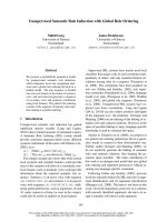
of sentence to you is highly weighted. Finally, Fig-
ure 2 illustrates how Model 4 (left) and our discrimi-
native model (right) align an English-Urdu sentence
pair (the English side is being conditioned on in both
models). A reflex of Urdu’s head-final word order
is seen in the list of most highly weighted bigrams,
where a path through the English source where verbs
that transition to end-of-sentence periods are predic-
tive of good translations into Urdu.
Table 5: The most highly weighted source path bigram
features in the English-Czech, -Chinese, and -Urdu mod-
els.
Bigram θ
k
. /s 3.08
like like 1.19
one of 1.06
” . 0.95
that that 0.92
is but 0.92
since since 0.84
s when 0.83
, how 0.83
, not 0.83
Bigram θ
k
. /s 2.67
? ? 2.25
s please 2.01

much ? 1.61
s if 1.58
thank you 1.47
s sorry 1.46
s you 1.45
please like 1.24
s this 1.19
Bigram θ
k
. /s 1.87
s this 1.24
will . 1.17
are . 1.16
is . 1.09
is that 1.00
have . 0.97
has . 0.96
was . 0.91
will /s 0.88
6 Related Work
The literature contains numerous descriptions of dis-
criminative approaches to word alignment motivated
by the desire to be able to incorporate multiple,
overlapping knowledge sources (Ayan et al., 2005;
Moore, 2005; Taskar et al., 2005; Blunsom and
Cohn, 2006; Haghighi et al., 2009; Liu et al., 2010;
DeNero and Klein, 2010; Setiawan et al., 2010).
This body of work has been an invaluable source
of useful features. Several authors have dealt with
the problem training log-linear models in an unsu-

416
IBM Model 4 alignment Our model's alignment
Figure 2: Example English-Urdu alignment under IBM Model 4 (left) and our discriminative model (right). Model
4 displays two characteristic errors: garbage collection and an overly-strong monotonicity bias. Whereas our model
does not exhibit these problems, and in fact, makes no mistakes in the alignment.
pervised setting. The contrastive estimation tech-
nique proposed by Smith and Eisner (2005) is glob-
ally normalized (and thus capable of dealing with ar-
bitrary features), and closely related to the model we
developed; however, they do not discuss the problem
of word alignment. Berg-Kirkpatrick et al. (2010)
learn locally normalized log-linear models in a gen-
erative setting. Globally normalized discriminative
models with latent variables (Quattoni et al., 2004)
have been used for a number of language processing
problems, including MT (Dyer and Resnik, 2010;
Blunsom et al., 2008a). However, this previous
work relied on translation grammars constructed us-
ing standard generative word alignment processes.
7 Future Work
While we have demonstrated that this model can be
substantially useful, it is limited in some important
ways which are being addressed in ongoing work.
First, training is expensive, and we are exploring al-
ternatives to the conditional likelihood objective that
is currently used, such as contrastive neighborhoods
advocated by (Smith and Eisner, 2005). Addition-
ally, there is much evidence that non-local features
like the source word fertility are (cf. IBM Model 3)
useful for translation and alignment modeling. To be

truly general, it must be possible to utilize such fea-
tures. Unfortunately, features like this that depend
on global properties of the alignment vector, a, make
the inference problem NP-hard, and approximations
are necessary. Fortunately, there is much recent
work on approximate inference techniques for incor-
porating nonlocal features (Blunsom et al., 2008b;
Gimpel and Smith, 2009; Cromi
`
eres and Kurohashi,
2009; Weiss and Taskar, 2010), suggesting that this
problem too can be solved using established tech-
niques.
8 Conclusion
We have introduced a globally normalized, log-
linear lexical translation model that can be trained
discriminatively using only parallel sentences,
which we apply to the problem of word alignment.
Our approach addresses two important shortcomings
of previous work: (1) that local normalization of
generative models constrains the features that can be
used, and (2) that previous discriminatively trained
word alignment models required supervised align-
ments. According to a variety of measures in a vari-
ety of translation tasks, this model produces superior
alignments to generative approaches. Furthermore,
the features learned by our model reveal interesting
characteristics of the language pairs being modeled.
Acknowledgments
This work was supported in part by the DARPA GALE

program; the U. S. Army Research Laboratory and the
U. S. Army Research Office under contract/grant num-
417
ber W911NF-10-1-0533; and the National Science Foun-
dation through grants IIS-0844507, IIS-0915187, IIS-
0713402, and IIS-0915327 and through TeraGrid re-
sources provided by the Pittsburgh Supercomputing Cen-
ter under grant number TG-DBS110003. We thank
Ond
ˇ
rej Bojar for providing the Czech-English alignment
data, and three anonymous reviewers for their detailed
suggestions and comments on an earlier draft of this pa-
per.
References
N. F. Ayan, B. J. Dorr, and C. Monz. 2005. NeurAlign:
combining word alignments using neural networks. In
Proc. of HLT-EMNLP.
T. Berg-Kirkpatrick, A. Bouchard-C
ˆ
ot
´
e, J. DeNero, and
D. Klein. 2010. Painless unsupervised learning with
features. In Proc. of NAACL.
P. Blunsom and T. Cohn. 2006. Discriminative word
alignment with conditional random fields. In Proc. of
ACL.
P. Blunsom, T. Cohn, and M. Osborne. 2008a. A dis-
criminative latent variable model for statistical ma-

chine translation. In Proc. of ACL-HLT.
P. Blunsom, T. Cohn, and M. Osborne. 2008b. Proba-
bilistic inference for machine translation. In Proc. of
EMNLP 2008.
O. Bojar and M. Prokopov
´
a. 2006. Czech-English word
alignment. In Proc. of LREC.
P. F. Brown, V. J. Della Pietra, S. A. Della Pietra, and
R. L. Mercer. 1993. The mathematics of statistical
machine translation: parameter estimation. Computa-
tional Linguistics, 19(2):263–311.
D. Chiang. 2007. Hierarchical phrase-based translation.
Computational Linguistics, 33(2):201–228.
J. Clark, C. Dyer, A. Lavie, and N. A. Smith. 2011. Bet-
ter hypothesis testing for statistical machine transla-
tion: Controlling for optimizer instability. In Proc. of
ACL.
F. Cromi
`
eres and S. Kurohashi. 2009. An alignment al-
gorithm using belief propagation and a structure-based
distortion model. In Proc. of EACL.
J. DeNero and D. Klein. 2010. Discriminative modeling
of extraction sets for machine translation. In Proc. of
ACL.
L. R. Dice. 1945. Measures of the amount of eco-
logic association between species. Journal of Ecology,
26:297–302.
C. Dyer and P. Resnik. 2010. Context-free reordering,

finite-state translation. In Proc. of NAACL.
C. Dyer, A. Lopez, J. Ganitkevitch, J. Weese, F. Ture,
P. Blunsom, H. Setiawan, V. Eidelman, and P. Resnik.
2010. cdec: A decoder, alignment, and learning
framework for finite-state and context-free translation
models. In Proc. of ACL (demonstration session).
A. Fraser. 2007. Improved Word Alignments for Statis-
tical Machine Translation. Ph.D. thesis, University of
Southern California.
K. Gimpel and N. A. Smith. 2009. Cube summing, ap-
proximate inference with non-local features, and dy-
namic programming without semirings. In Proc. of
EACL.
N. Habash and F. Sadat. 2006. Arabic preprocessing
schemes for statistical machine translation. In Proc. of
NAACL, New York.
A. Haghighi, J. Blitzer, J. DeNero, and D. Klein. 2009.
Better word alignments with supervised ITG models.
In Proc. of ACL-IJCNLP.
P. Koehn, F. J. Och, and D. Marcu. 2003. Statistical
phrase-based translation. In Proc. of NAACL.
D. Koller and N. Friedman. 2009. Probabilistic Graphi-
cal Models: Principles and Techniques. MIT Press.
S. Kumar, W. Macherey, C. Dyer, and F. Och. 2009. Effi-
cient minimum error rate training and minimum bayes-
risk decoding for translation hypergraphs and lattices.
In Proc. of ACL-IJCNLP.
J. Lafferty, A. McCallum, and F. Pereira. 2001. Con-
ditional random fields: Probabilistic models for seg-
menting and labeling sequence data. In Proc. of ICML.

A. Lavie and M. Denkowski. 2009. The METEOR metric
for automatic evaluation of machine translation. Ma-
chine Translation Journal, 23(2–3):105–115.
P. Liang and D. Klein. 2009. Online EM for unsuper-
vised models. In Proc. of NAACL.
Y. Liu, T. Xia, X. Xiao, and Q. Liu. 2009. Weighted
alignment matrices for statistical machine translation.
In Proc. of EMNLP.
Y. Liu, Q. Liu, and S. Lin. 2010. Discriminative word
alignment by linear modeling. Computational Lin-
guistics, 36(3):303–339.
A. Lopez. 2008. Tera-scale translation models via pat-
tern matching. In Proc. of COLING.
R. Mihalcea and T. Pedersen. 2003. An evaluation exer-
cise for word alignment. In Proc. of the Workshop on
Building and Using Parallel Texts.
R. C. Moore. 2005. A discriminative framework for
bilingual word alignment. In Proc. of HLT-EMNLP.
F. Och and H. Ney. 2003. A systematic comparison of
various statistical alignment models. Computational
Linguistics, 29(1):19–51.
F. Och. 1999. An efficient method for determining bilin-
gual word classes. In Proc. of EACL.
K. Papineni, S. Roukos, T. Ward, and W J. Zhu. 2002.
BLEU: a method for automatic evaluation of machine
translation. In Proc. of ACL.
418
A. Quattoni, M. Collins, and T. Darrell. 2004. Condi-
tional random fields for object recognition. In NIPS
17.

H. Setiawan, C. Dyer, and P. Resnik. 2010. Discrimina-
tive word alignment with a function word reordering
model. In Proc. of EMNLP.
N. A. Smith and J. Eisner. 2005. Contrastive estimation:
training log-linear models on unlabeled data. In Proc.
of ACL.
M. Snover, B. J. Dorr, R. Schwartz, L. Micciulla, and
J. Makhoul. 2006. A study of translation edit rate
with targeted human annotation. In Proc. of AMTA.
T. Takezawa, E. Sumita, F. Sugaya, H. Yamamoto, and
S. Yamamoto. 2002. Toward a broad-coverage bilin-
gual corpus for speech translation of travel conversa-
tions in the real world. In Proc. of LREC.
B. Taskar, S. Lacoste-Julien, and D. Klein. 2005. A dis-
criminative matching approach to word alignment. In
Proc. of HLT-EMNLP.
Y. Tsuruoka, J. Tsujii, and S. Ananiadou. 2009. Stochas-
tic gradient descent training for l
1
-regularized log-
linear models with cumulative penalty. In Proc. of
ACL-IJCNLP.
A. Venugopal, A. Zollmann, N. A. Smith, and S. Vogel.
2008. Wider pipelines: n-best alignments and parses
in MT training. In Proc. of AMTA.
S. Vogel, H. Ney, and C. Tillmann. 1996. HMM-based
word alignment in statistical translation. In Proc. of
COLING.
D. Weiss and B. Taskar. 2010. Structured prediction cas-
cades. In Proc. of AISTATS.

419