Báo cáo khoa học: "Forest Reranking: Discriminative Parsing with Non-Local Features∗" docx
Bạn đang xem bản rút gọn của tài liệu. Xem và tải ngay bản đầy đủ của tài liệu tại đây (263.16 KB, 9 trang )
Proceedings of ACL-08: HLT, pages 586–594,
Columbus, Ohio, USA, June 2008.
c
2008 Association for Computational Linguistics
Forest Reranking: Discriminative Parsing with Non-Local Features
∗
Liang Huang
University of Pennsylvania
Philadelphia, PA 19104
Abstract
Conventional n-best reranking techniques of-
ten suffer from the limited scope of the n-
best list, which rules out many potentially
good alternatives. We instead propose forest
reranking, a method that reranks a packed for-
est of exponentially many parses. Since ex-
act inference is intractable with non-local fea-
tures, we present an approximate algorithm in-
spired by forest rescoring that makes discrim-
inative training practical over the whole Tree-
bank. Our final result, an F-score of 91.7, out-
performs both 50-best and 100-best reranking
baselines, and is better than any previously re-
ported systems trained on the Treebank.
1 Introduction
Discriminative reranking has become a popular
technique for many NLP problems, in particular,
parsing (Collins, 2000) and machine translation
(Shen et al., 2005). Typically, this method first gen-
erates a list of top-n candidates from a baseline sys-
tem, and then reranks this n-best list with arbitrary
features that are not computable or intractable to
compute within the baseline system. But despite its
apparent success, there remains a major drawback:
this method suffers from the limited scope of the n-
best list, which rules out many potentially good al-
ternatives. For example 41% of the correct parses
were not in the candidates of ∼30-best parses in
(Collins, 2000). This situation becomes worse with
longer sentences because the number of possible in-
terpretations usually grows exponentially with the
∗
Part of this work was done while I was visiting Institute
of Computing Technology, Beijing, and I thank Prof. Qun Liu
and his lab for hosting me. I am also grateful to Dan Gildea and
Mark Johnson for inspirations, Eugene Charniak for help with
his parser, and Wenbin Jiang for guidance on perceptron aver-
aging. This project was supported by NSF ITR EIA-0205456.
local non-local
conventional reranking only at the root
DP-based discrim. parsing
exact N/A
this work: forest-reranking exact on-the-fly
Table 1: Comparison of various approaches for in-
corporating local and non-local features.
sentence length. As a result, we often see very few
variations among the n-best trees, for example, 50-
best trees typically just represent a combination of 5
to 6 binary ambiguities (since 2
5
< 50 < 2
6
).
Alternatively, discriminative parsing is tractable
with exact and efficient search based on dynamic
programming (DP) if all features are restricted to be
local, that is, only looking at a local window within
the factored search space (Taskar et al., 2004; Mc-
Donald et al., 2005). However, we miss the benefits
of non-local features that are not representable here.
Ideally, we would wish to combine the merits of
both approaches, where an efficient inference algo-
rithm could integrate both local and non-local fea-
tures. Unfortunately, exact search is intractable (at
least in theory) for features with unbounded scope.
So we propose forest reranking, a technique inspired
by forest rescoring (Huang and Chiang, 2007) that
approximately reranks the packed forest of expo-
nentially many parses. The key idea is to compute
non-local features incrementally from bottom up, so
that we can rerank the n-best subtrees at all internal
nodes, instead of only at the root node as in conven-
tional reranking (see Table 1). This method can thus
be viewed as a step towards the integration of dis-
criminative reranking with traditional chart parsing.
Although previous work on discriminative pars-
ing has mainly focused on short sentences (≤ 15
words) (Taskar et al., 2004; Turian and Melamed,
2007), our work scales to the whole Treebank, where
586
VP
1,6
VBD
1,2
blah NP
2,6
NP
2,3
blah PP
3,6
b
e
2
e
1
Figure 1: A partial forest of the example sentence.
we achieved an F-score of 91.7, which is a 19% er-
ror reduction from the 1-best baseline, and outper-
forms both 50-best and 100-best reranking. This re-
sult is also better than any previously reported sys-
tems trained on the Treebank.
2 Packed Forests as Hypergraphs
Informally, a packed parse forest, or forest in short,
is a compact representation of all the derivations
(i.e., parse trees) for a given sentence under a
context-free grammar (Billot and Lang, 1989). For
example, consider the following sentence
0
I
1
saw
2
him
3
with
4
a
5
mirror
6
where the numbers between words denote string po-
sitions. Shown in Figure 1, this sentence has (at
least) two derivations depending on the attachment
of the prep. phrase PP
3,6
“with a mirror”: it can ei-
ther be attached to the verb “saw”,
VBD
1,2
NP
2,3
PP
3,6
VP
1,6
, (*)
or be attached to “him”, which will be further com-
bined with the verb to form the same VP as above.
These two derivations can be represented as a sin-
gle forest by sharing common sub-derivations. Such
a forest has a structure of a hypergraph (Klein and
Manning, 2001; Huang and Chiang, 2005), where
items like PP
3,6
are called nodes, and deductive
steps like (*) correspond to hyperedges.
More formally, a forest is a pair V, E, where V
is the set of nodes, and E the set of hyperedges. For
a given sentence w
1:l
= w
1
. . . w
l
, each node v ∈ V
is in the form of X
i,j
, which denotes the recogni-
tion of nonterminal X spanning the substring from
positions i through j (that is, w
i+1
. . . w
j
). Each hy-
peredge e ∈ E is a pair tails(e), head(e), where
head(e) ∈ V is the consequent node in the deduc-
tive step, and tails(e) ∈ V
∗
is the list of antecedent
nodes. For example, the hyperedge for deduction (*)
is notated:
e
1
= (VBD
1,2
, NP
2,3
, PP
3,6
), VP
1,6
We also denote IN (v) to be the set of incom-
ing hyperedges of node v, which represent the dif-
ferent ways of deriving v. For example, in the for-
est in Figure 1, IN (VP
1,6
) is {e
1
, e
2
}, with e
2
=
(VBD
1,2
, NP
2,6
), VP
1,6
. We call |e| the arity of
hyperedge e, which counts the number of tail nodes
in e. The arity of a hypergraph is the maximum ar-
ity over all hyperedges. A CKY forest has an arity
of 2, since the input grammar is required to be bi-
nary branching (cf. Chomsky Normal Form) to en-
sure cubic time parsing complexity. However, in this
work, we use forests from a Treebank parser (Char-
niak, 2000) whose grammar is often flat in many
productions. For example, the arity of the forest in
Figure 1 is 3. Such a Treebank-style forest is eas-
ier to work with for reranking, since many features
can be directly expressed in it. There is also a distin-
guished root node TOP in each forest, denoting the
goal item in parsing, which is simply S
0,l
where S is
the start symbol and l is the sentence length.
3 Forest Reranking
3.1 Generic Reranking with the Perceptron
We first establish a unified framework for parse
reranking with both n-best lists and packed forests.
For a given sentence s, a generic reranker selects
the best parse ˆy among the set of candidates cand(s)
according to some scoring function:
ˆy = argmax
y∈cand (s)
score(y) (1)
In n-best reranking, cand(s) is simply a set of
n-best parses from the baseline parser, that is,
cand(s) = {y
1
, y
2
, . . . , y
n
}. Whereas in forest
reranking, cand(s) is a forest implicitly represent-
ing the set of exponentially many parses.
As usual, we define the score of a parse y to be
the dot product between a high dimensional feature
representation and a weight vector w:
score(y) = w · f(y) (2)
587
where the feature extractor f is a vector of d func-
tions f = (f
1
, . . . , f
d
), and each feature f
j
maps
a parse y to a real number f
j
(y). Following (Char-
niak and Johnson, 2005), the first feature f
1
(y) =
log Pr(y) is the log probability of a parse from the
baseline generative parser, while the remaining fea-
tures are all integer valued, and each of them counts
the number of times that a particular configuration
occurs in parse y. For example, one such feature
f
2000
might be a question
“how many times is a VP of length 5 surrounded
by the word ‘has’ and the period? ”
which is an instance of the WordEdges feature (see
Figure 2(c) and Section 3.2 for details).
Using a machine learning algorithm, the weight
vector w can be estimated from the training data
where each sentence s
i
is labelled with its cor-
rect (“gold-standard”) parse y
∗
i
. As for the learner,
Collins (2000) uses the boosting algorithm and
Charniak and Johnson (2005) use the maximum en-
tropy estimator. In this work we use the averaged
perceptron algorithm (Collins, 2002) since it is an
online algorithm much simpler and orders of magni-
tude faster than Boosting and MaxEnt methods.
Shown in Pseudocode 1, the perceptron algo-
rithm makes several passes over the whole train-
ing data, and in each iteration, for each sentence s
i
,
it tries to predict a best parse ˆy
i
among the candi-
dates cand (s
i
) using the current weight setting. In-
tuitively, we want the gold parse y
∗
i
to be picked, but
in general it is not guaranteed to be within cand(s
i
),
because the grammar may fail to cover the gold
parse, and because the gold parse may be pruned
away due to the limited scope of cand(s
i
). So we
define an oracle parse y
+
i
to be the candidate that
has the highest Parseval F-score with respect to the
gold tree y
∗
i
:
1
y
+
i
argmax
y∈cand (s
i
)
F (y, y
∗
i
) (3)
where function F returns the F-score. Now we train
the reranker to pick the oracle parses as often as pos-
sible, and in case an error is made (line 6), perform
an update on the weight vector (line 7), by adding
the difference between two feature representations.
1
If one uses the gold y
∗
i
for oracle y
+
i
, the perceptron will
continue to make updates towards something unreachable even
when the decoder has picked the best possible candidate.
Pseudocode 1 Perceptron for Generic Reranking
1: Input: Training examples {cand(s
i
), y
+
i
}
N
i=1
⊲ y
+
i
is the
oracle tree for s
i
among cand(s
i
)
2: w ← 0 ⊲ initial weights
3: for t ← 1 . . . T do ⊲ T iterations
4: for i ← 1 . . . N do
5: ˆy = argmax
y∈cand(s
i
)
w · f(y)
6: if ˆy = y
+
i
then
7: w ← w + f(y
+
i
) − f (ˆy)
8: return w
In n-best reranking, since all parses are explicitly
enumerated, it is trivial to compute the oracle tree.
2
However, it remains widely open how to identify the
forest oracle. We will present a dynamic program-
ming algorithm for this problem in Sec. 4.1.
We also use a refinement called “averaged param-
eters” where the final weight vector is the average of
weight vectors after each sentence in each iteration
over the training data. This averaging effect has been
shown to reduce overfitting and produce much more
stable results (Collins, 2002).
3.2 Factorizing Local and Non-Local Features
A key difference between n-best and forest rerank-
ing is the handling of features. In n-best reranking,
all features are treated equivalently by the decoder,
which simply computes the value of each one on
each candidate parse. However, for forest reranking,
since the trees are not explicitly enumerated, many
features can not be directly computed. So we first
classify features into local and non-local, which the
decoder will process in very different fashions.
We define a feature f to be local if and only if
it can be factored among the local productions in a
tree, and non-local if otherwise. For example, the
Rule feature in Fig. 2(a) is local, while the Paren-
tRule feature in Fig. 2(b) is non-local. It is worth
noting that some features which seem complicated
at the first sight are indeed local. For example, the
WordEdges feature in Fig. 2(c), which classifies
a node by its label, span length, and surrounding
words, is still local since all these information are
encoded either in the node itself or in the input sen-
tence. In contrast, it would become non-local if we
replace the surrounding words by surrounding POS
2
In case multiple candidates get the same highest F-score,
we choose the parse with the highest log probability from the
baseline parser to be the oracle parse (Collins, 2000).
588
VP
VBD NP PP
S
VP
VBD NP PP
VP
VBZ
has
NP
|← 5 words →|
.
.
VP
VBD
saw
NP
DT
the
(a) Rule (local) (b) ParentRule (non-local) (c) WordEdges (local) (d) NGramTree (non-local)
VP → VBD NP PP VP → VBD NP PP | S NP 5 has . VP (VBD saw) (NP (DT the))
Figure 2: Illustration of some example features. Shaded nodes denote information included in the feature.
tags, which are generated dynamically.
More formally, we split the feature extractor f =
(f
1
, . . . , f
d
) into f = (f
L
; f
N
) where f
L
and f
N
are
the local and non-local features, respectively. For the
former, we extend their domains from parses to hy-
peredges, where f(e) returns the value of a local fea-
ture f ∈ f
L
on hyperedge e, and its value on a parsey
factors across the hyperedges (local productions),
f
L
(y) =
e∈y
f
L
(e) (4)
and we can pre-compute f
L
(e) for each e in a forest.
Non-local features, however, can not be pre-
computed, but we still prefer to compute them as
early as possible, which we call “on-the-fly” com-
putation, so that our decoder can be sensitive to them
at internal nodes. For instance, the NGramTree fea-
ture in Fig. 2 (d) returns the minimum tree fragement
spanning a bigram, in this case “saw” and “the”, and
should thus be computed at the smallest common an-
cestor of the two, which is the VP node in this ex-
ample. Similarly, the ParentRule feature in Fig. 2
(b) can be computed when the S subtree is formed.
In doing so, we essentially factor non-local features
across subtrees, where for each subtree y
′
in a parse
y, we define a unit feature
˚
f(y
′
) to be the part of
f(y) that are computable within y
′
, but not com-
putable in any (proper) subtree of y
′
. Then we have:
f
N
(y) =
y
′
∈y
˚
f
N
(y
′
) (5)
Intuitively, we compute the unit non-local fea-
tures at each subtree from bottom-up. For example,
for the binary-branching node A
i,k
in Fig. 3, the
A
i,k
B
i,j
w
i
. . . w
j−1
C
j,k
w
j
. . . w
k−1
Figure 3: Example of the unit NGramTree feature
at node A
i,k
: A (B . . . w
j−1
) (C . . . w
j
) .
unit NGramTree instance is for the pair w
j−1
, w
j
on the boundary between the two subtrees, whose
smallest common ancestor is the current node. Other
unit NGramTree instances within this span have al-
ready been computed in the subtrees, except those
for the boundary words of the whole node, w
i
and
w
k−1
, which will be computed when this node is fur-
ther combined with other nodes in the future.
3.3 Approximate Decoding via Cube Pruning
Before moving on to approximate decoding with
non-local features, we first describe the algorithm
for exact decoding when only local features are
present, where many concepts and notations will be
re-used later. We will use D(v) to denote the top
derivations of node v, where D
1
(v) is its 1-best
derivation. We also use the notation e, j to denote
the derivation along hyperedge e, using the j
i
th sub-
derivation for tail u
i
, so e, 1 is the best deriva-
tion along e. The exact decoding algorithm, shown
in Pseudocode 2, is an instance of the bottom-up
Viterbi algorithm, which traverses the hypergraph in
a topological order, and at each node v, calculates
its 1-best derivation using each incoming hyperedge
e ∈ IN (v). The cost of e, c(e), is the score of its
589
Pseudocode 2 Exact Decoding with Local Features
1: function VITERBI(V, E)
2: for v ∈ V in topological order do
3: for e ∈ IN (v) do
4: c(e) ← w · f
L
(e) +
P
u
i
∈tails(e)
c(D
1
(u
i
))
5: if c(e) > c(D
1
(v)) then ⊲ better derivation?
6: D
1
(v) ← e, 1
7: c(D
1
(v)) ← c(e)
8: return D
1
(TOP)
Pseudocode 3 Cube Pruning for Non-local Features
1: function CUBE(V, E)
2: for v ∈ V in topological order do
3: KBEST(v)
4: return D
1
(TOP)
5: procedure KBEST(v)
6: heap ← ∅; buf ← ∅
7: for e ∈ IN (v) do
8: c(e, 1) ← EVAL(e, 1) ⊲ extract unit features
9: append e, 1 to heap
10: HEAPIFY(heap) ⊲ prioritized frontier
11: while |heap| > 0 and |buf | < k do
12: item ← POP-MAX(heap) ⊲ extract next-best
13: append item to buf
14: PUSHSUCC(item, heap)
15: sort buf to D(v)
16: procedure PUSHSUCC(e, j, heap)
17: e is v → u
1
. . . u
|e|
18: for i in 1 . . . |e| do
19: j
′
← j + b
i
⊲ b
i
is 1 only on the ith dim.
20: if |D(u
i
)| ≥ j
′
i
then ⊲ enough sub-derivations?
21: c(e, j
′
) ← EVAL(e, j
′
) ⊲ unit features
22: PUSH(e, j
′
, heap)
23: function EVAL(e, j)
24: e is v → u
1
. . . u
|e|
25: return w · f
L
(e) + w ·
˚
f
N
(e, j) +
P
i
c(D
j
i
(u
i
))
(pre-computed) local features w · f
L
(e). This algo-
rithm has a time complexity of O(E), and is almost
identical to traditional chart parsing, except that the
forest might be more than binary-branching.
For non-local features, we adapt cube pruning
from forest rescoring (Chiang, 2007; Huang and
Chiang, 2007), since the situation here is analogous
to machine translation decoding with integrated lan-
guage models: we can view the scores of unit non-
local features as the language model cost, computed
on-the-fly when combining sub-constituents.
Shown in Pseudocode 3, cube pruning works
bottom-up on the forest, keeping a beam of at most k
derivations at each node, and uses the k-best pars-
ing Algorithm 2 of Huang and Chiang (2005) to
speed up the computation. When combining the sub-
derivations along a hyperedge e to form a new sub-
tree y
′
= e, j, we also compute its unit non-local
feature values
˚
f
N
(e, j) (line 25). A priority queue
(heap in Pseudocode 3) is used to hold the candi-
dates for the next-best derivation, which is initial-
ized to the set of best derivations along each hyper-
edge (lines 7 to 9). Then at each iteration, we pop
the best derivation (lines 12), and push its succes-
sors back into the priority queue (line 14). Analo-
gous to the language model cost in forest rescoring,
the unit feature cost here is a non-monotonic score in
the dynamic programming backbone, and the deriva-
tions may thus be extracted out-of-order. So a buffer
buf is used to hold extracted derivations, which is
sorted at the end (line 15) to form the list of top-k
derivations D(v) of node v. The complexity of this
algorithm is O(E + V k log kN ) (Huang and Chi-
ang, 2005), where O(N ) is the time for on-the-fly
feature extraction for each subtree, which becomes
the bottleneck in practice.
4 Supporting Forest Algorithms
4.1 Forest Oracle
Recall that the Parseval F-score is the harmonic
mean of labelled precision P and labelled recall R:
F (y, y
∗
)
2P R
P + R
=
2|y ∩ y
∗
|
|y| + |y
∗
|
(6)
where |y| and |y
∗
| are the numbers of brackets in the
test parse and gold parse, respectively, and |y ∩ y
∗
|
is the number of matched brackets. Since the har-
monic mean is a non-linear combination, we can not
optimize the F-scores on sub-forests independently
with a greedy algorithm. In other words, the optimal
F-score tree in a forest is not guaranteed to be com-
posed of two optimal F-score subtrees.
We instead propose a dynamic programming al-
gorithm which optimizes the number of matched
brackets for a given number of test brackets. For ex-
ample, our algorithm will ask questions like,
“when a test parse has 5 brackets, what is the
maximum number of matched brackets?”
More formally, at each node v, we compute an ora-
cle function ora[v] : N → N, which maps an integer
t to ora[v](t), the max. number of matched brackets
590
Pseudocode 4 Forest Oracle Algorithm
1: function ORACLE(V, E, y
∗
)
2: for v ∈ V in topological order do
3: for e ∈ BS(v) do
4: e is v → u
1
u
2
. . . u
|e|
5: ora[v] ← ora[v] ⊕ (⊗
i
ora[u
i
])
6: ora[v] ← ora[v] ⇑ (1, 1
v∈y
∗
)
7: return F (y
+
, y
∗
) = max
t
2·ora [TOP](t)
t+|y
∗
|
⊲ oracle F
1
for all parses y
v
of node v with exactly t brackets:
ora[v](t) max
y
v
:|y
v
|=t
|y
v
∩ y
∗
| (7)
When node v is combined with another node u
along a hyperedge e = (v, u), w, we need to com-
bine the two oracle functions ora[v] and ora[u] by
distributing the test brackets of w between v and u,
and optimize the number of matched bracktes. To
do this we define a convolution operator ⊗ between
two functions f and g:
(f ⊗ g)(t) max
t
1
+t
2
=t
f(t
1
) + g(t
2
) (8)
For instance:
t f(t)
2 1
3
2
⊗
t
g(t)
4 4
5
4
=
t
(f ⊗ g)(t)
6 5
7
6
8
6
The oracle function for the head node w is then
ora[w](t) = (ora[v] ⊗ ora[u])(t − 1) + 1
w∈y
∗
(9)
where 1 is the indicator function, returning 1 if node
w is found in the gold tree y
∗
, in which case we
increment the number of matched brackets. We can
also express Eq. 9 in a purely functional form
ora[w] = (ora[v] ⊗ ora[u]) ⇑ (1, 1
w∈y
∗
) (10)
where ⇑ is a translation operator which shifts a
function along the axes:
(f ⇑ (a, b))(t) f(t − a) + b (11)
Above we discussed the case of one hyperedge. If
there is another hyperedge e
′
deriving node w, we
also need to combine the resulting oracle functions
from both hyperedges, for which we define a point-
wise addition operator ⊕:
(f ⊕ g)(t) max{f(t), g(t)} (12)
Shown in Pseudocode 4, we perform these com-
putations in a bottom-up topological order, and fi-
nally at the root node TOP, we can compute the best
global F-score by maximizing over different num-
bers of test brackets (line 7). The oracle tree y
+
can
be recursively restored by keeping backpointers for
each ora[v](t), which we omit in the pseudocode.
The time complexity of this algorithm for a sen-
tence of l words is O(|E| · l
2(a−1)
) where a is the
arity of the forest. For a CKY forest, this amounts
to O(l
3
· l
2
) = O(l
5
), but for general forests like
those in our experiments the complexities are much
higher. In practice it takes on average 0.05 seconds
for forests pruned by p = 10 (see Section 4.2), but
we can pre-compute and store the oracle for each
forest before training starts.
4.2 Forest Pruning
Our forest pruning algorithm (Jonathan Graehl, p.c.)
is very similar to the method based on marginal
probability (Charniak and Johnson, 2005), except
that ours prunes hyperedges as well as nodes. Ba-
sically, we use an Inside-Outside algorithm to com-
pute the Viterbi inside cost β(v) and the Viterbi out-
side cost α(v) for each node v, and then compute the
merit αβ(e) for each hyperedge:
αβ(e) = α(head(e)) +
u
i
∈tails(e)
β(u
i
) (13)
Intuitively, this merit is the cost of the best deriva-
tion that traverses e, and the difference δ(e) =
αβ(e) − β(TOP) can be seen as the distance away
from the globally best derivation. We prune away
all hyperedges that have δ(e) > p for a thresh-
old p. Nodes with all incoming hyperedges pruned
are also pruned. The key difference from (Charniak
and Johnson, 2005) is that in this algorithm, a node
can “partially” survive the beam, with a subset of its
hyperedges pruned. In practice, this method prunes
on average 15% more hyperedges than their method.
5 Experiments
We compare the performance of our forest reranker
against n-best reranking on the Penn English Tree-
bank (Marcus et al., 1993). The baseline parser is
the Charniak parser, which we modified to output a
591
Local instances Non-Local instances
Rule 10, 851 ParentRule 18,019
Word 20, 328 WProj 27, 417
WordEdges 454, 101 Heads 70,013
CoLenPar 22 HeadTree 67, 836
Bigram
⋄
10, 292 Heavy 1, 401
Trigram
⋄
24, 677 NGramTree 67, 559
HeadMod
⋄
12, 047 RightBranch 2
DistMod
⋄
16, 017
Total Feature Instances: 800, 582
Table 2: Features used in this work. Those with a
⋄
are from (Collins, 2000), and others are from (Char-
niak and Johnson, 2005), with simplifications.
packed forest for each sentence.
3
5.1 Data Preparation
We use the standard split of the Treebank: sections
02-21 as the training data (39832 sentences), sec-
tion 22 as the development set (1700 sentences), and
section 23 as the test set (2416 sentences). Follow-
ing (Charniak and Johnson, 2005), the training set is
split into 20 folds, each containing about 1992 sen-
tences, and is parsed by the Charniak parser with a
model trained on sentences from the remaining 19
folds. The development set and the test set are parsed
with a model trained on all 39832 training sentences.
We implemented both n-best and forest reranking
systems in Python and ran our experiments on a 64-
bit Dual-Core Intel Xeon with 3.0GHz CPUs. Our
feature set is summarized in Table 2, which closely
follows Charniak and Johnson (2005), except that
we excluded the non-local features Edges, NGram,
and CoPar, and simplified Rule and NGramTree
features, since they were too complicated to com-
pute.
4
We also added four unlexicalized local fea-
tures from Collins (2000) to cope with data-sparsity.
Following Charniak and Johnson (2005), we ex-
tracted the features from the 50-best parses on the
training set (sec. 02-21), and used a cut-off of 5 to
prune away low-count features. There are 0.8M fea-
tures in our final set, considerably fewer than that
of Charniak and Johnson which has about 1.3M fea-
3
This is a relatively minor change to the Charniak parser,
since it implements Algorithm 3 of Huang and Chiang (2005)
for efficient enumeration of n-best parses, which requires stor-
ing the forest. The modified parser and related scripts for han-
dling forests (e.g. oracles) will be available on my homepage.
4
In fact, our Rule and ParentRule features are two special
cases of the original Rule feature in (Charniak and Johnson,
2005). We also restricted NGramTree to be on bigrams only.
89.0
91.0
93.0
95.0
97.0
99.0
0 500 1000 1500 2000
Parseval F-score (%)
average # of hyperedges or brackets per sentence
p=10 p=20
n=10
n=50
n=100
1-best
forest oracle
n-best oracle
Figure 4: Forests (shown with various pruning
thresholds) enjoy higher oracle scores and more
compact sizes than n-best lists (on sec 23).
tures in the updated version.
5
However, our initial
experiments show that, even with this much simpler
feature set, our 50-best reranker performed equally
well as theirs (both with an F-score of 91.4, see Ta-
bles 3 and 4). This result confirms that our feature
set design is appropriate, and the averaged percep-
tron learner is a reasonable candidate for reranking.
The forests dumped from the Charniak parser are
huge in size, so we use the forest pruning algorithm
in Section 4.2 to prune them down to a reasonable
size. In the following experiments we use a thresh-
old of p = 10, which results in forests with an av-
erage number of 123.1 hyperedges per forest. Then
for each forest, we annotate its forest oracle, and
on each hyperedge, pre-compute its local features.
6
Shown in Figure 4, these forests have an forest or-
acle of 97.8, which is 1.1% higher than the 50-best
oracle (96.7), and are 8 times smaller in size.
5.2 Results and Analysis
Table 3 compares the performance of forest rerank-
ing against standard n-best reranking. For both sys-
tems, we first use only the local features, and then
all the features. We use the development set to deter-
mine the optimal number of iterations for averaged
perceptron, and report the F
1
score on the test set.
With only local features, our forest reranker achieves
an F-score of 91.25, and with the addition of non-
5
We follow
this version as it corrects some bugs from their 2005 paper
which leads to a 0.4% increase in performance (see Table 4).
6
A subset of local features, e.g. WordEdges, is independent
of which hyperedge the node takes in a derivation, and can thus
be annotated on nodes rather than hyperedges. We call these
features node-local, which also include part of Word features.
592
baseline: 1-best Charniak parser 89.72
n-best reranking
features n pre-comp. training F
1
%
local 50 1.7G / 16h 3 × 0.1h 91.28
all 50 2.4G / 19h 4 × 0.3h 91.43
all 100 5.3G / 44h 4 × 0.7h 91.49
forest reranking (p = 10)
features k pre-comp. training F
1
%
local -
1.2G / 2.9h
3 × 0.8h 91.25
all 15 4 × 6.1h 91.69
Table 3: Forest reranking compared to n-best rerank-
ing on sec. 23. The pre-comp. column is for feature
extraction, and training column shows the number
of perceptron iterations that achieved best results on
the dev set, and average time per iteration.
local features, the accuracy rises to 91.69 (with beam
size k = 15), which is a 0.26% absolute improve-
ment over 50-best reranking.
7
This improvement might look relatively small, but
it is much harder to make a similar progress with
n-best reranking. For example, even if we double
the size of the n-best list to 100, the performance
only goes up by 0.06% (Table 3). In fact, the 100-
best oracle is only 0.5% higher than the 50-best one
(see Fig. 4). In addition, the feature extraction step
in 100-best reranking produces huge data files and
takes 44 hours in total, though this part can be paral-
lelized.
8
On two CPUs, 100-best reranking takes 25
hours, while our forest-reranker can also finish in 26
hours, with a much smaller disk space. Indeed, this
demonstrates the severe redundancies as another dis-
advantage of n-best lists, where many subtrees are
repeated across different parses, while the packed
forest reduces space dramatically by sharing com-
mon sub-derivations (see Fig. 4).
To put our results in perspective, we also compare
them with other best-performing systems in Table 4.
Our final result (91.7) is better than any previously
reported system trained on the Treebank, although
7
It is surprising that 50-best reranking with local features
achieves an even higher F-score of 91.28, and we suspect this is
due to the aggressive updates and instability of the perceptron,
as we do observe the learning curves to be non-monotonic. We
leave the use of more stable learning algorithms to future work.
8
The n-best feature extraction already uses relative counts
(Johnson, 2006), which reduced file sizes by at least a factor 4.
type system F
1
%
D
Collins (2000) 89.7
Henderson (2004) 90.1
Charniak and Johnson (2005) 91.0
updated (Johnson, 2006) 91.4
this work 91.7
G
Bod (2003) 90.7
Petrov and Klein (2007) 90.1
S McClosky et al. (2006) 92.1
Table 4: Comparison of our final results with other
best-performing systems on the whole Section 23.
Types D, G, and S denote discriminative, generative,
and semi-supervised approaches, respectively.
McClosky et al. (2006) achieved an even higher ac-
cuarcy (92.1) by leveraging on much larger unla-
belled data. Moreover, their technique is orthogonal
to ours, and we suspect that replacing their n-best
reranker by our forest reranker might get an even
better performance. Plus, except for n-best rerank-
ing, most discriminative methods require repeated
parsing of the training set, which is generally im-
pratical (Petrov and Klein, 2008). Therefore, pre-
vious work often resorts to extremely short sen-
tences (≤ 15 words) or only looked at local fea-
tures (Taskar et al., 2004; Henderson, 2004; Turian
and Melamed, 2007). In comparison, thanks to the
efficient decoding, our work not only scaled to the
whole Treebank, but also successfully incorporated
non-local features, which showed an absolute im-
provement of 0.44% over that of local features alone.
6 Conclusion
We have presented a framework for reranking on
packed forests which compactly encodes many more
candidates than n-best lists. With efficient approx-
imate decoding, perceptron training on the whole
Treebank becomes practical, which can be done in
about a day even with a Python implementation. Our
final result outperforms both 50-best and 100-best
reranking baselines, and is better than any previ-
ously reported systems trained on the Treebank. We
also devised a dynamic programming algorithm for
forest oracles, an interesting problem by itself. We
believe this general framework could also be applied
to other problems involving forests or lattices, such
as sequence labeling and machine translation.
593
References
Sylvie Billot and Bernard Lang. 1989. The struc-
ture of shared forests in ambiguous parsing. In
Proceedings of ACL ’89, pages 143–151.
Rens Bod. 2003. An efficient implementation of a
new DOP model. In Proceedings of EACL.
Eugene Charniak and Mark Johnson. 2005. Coarse-
to-fine-grained n-best parsing and discriminative
reranking. In Proceedings of the 43rd ACL.
Eugene Charniak. 2000. A maximum-entropy-
inspired parser. In Proceedings of NAACL.
David Chiang. 2007. Hierarchical phrase-
based translation. Computational Linguistics,
33(2):201–208.
Michael Collins. 2000. Discriminative reranking
for natural language parsing. In Proceedings of
ICML, pages 175–182.
Michael Collins. 2002. Discriminative training
methods for hidden markov models: Theory and
experiments with perceptron algorithms. In Pro-
ceedings of EMNLP.
James Henderson. 2004. Discriminative training of
a neural network statistical parser. In Proceedings
of ACL.
Liang Huang and David Chiang. 2005. Better k-
best Parsing. In Proceedings of the Ninth Interna-
tional Workshop on Parsing Technologies (IWPT-
2005).
Liang Huang and David Chiang. 2007. Forest
rescoring: Fast decoding with integrated language
models. In Proceedings of ACL.
Mark Johnson. 2006. Features of statisti-
cal parsers. Talk given at the Joint Mi-
crosoft Research and Univ. of Washing-
ton Computational Linguistics Colloquium.
/>uw06talk.pdf.
Dan Klein and Christopher D. Manning. 2001.
Parsing and Hypergraphs. In Proceedings of the
Seventh International Workshop on Parsing Tech-
nologies (IWPT-2001), 17-19 October 2001, Bei-
jing, China.
Mitchell P. Marcus, Beatrice Santorini, and
Mary Ann Marcinkiewicz. 1993. Building a
large annotated corpus of English: the Penn Tree-
bank. Computational Linguistics, 19:313–330.
David McClosky, Eugene Charniak, and Mark John-
son. 2006. Effective self-training for parsing. In
Proceedings of the HLT-NAACL, New York City,
USA, June.
Ryan McDonald, Koby Crammer, and Fernando
Pereira. 2005. Online large-margin training of
dependency parsers. In Proceedings of the 43rd
ACL.
Slav Petrov and Dan Klein. 2007. Improved infer-
ence for unlexicalized parsing. In Proceedings of
HLT-NAACL.
Slav Petrov and Dan Klein. 2008. Discriminative
log-linear grammars with latent variables. In Pro-
ceedings of NIPS 20.
Libin Shen, Anoop Sarkar, and Franz Josef Och.
2005. Discriminative reranking for machine
translation. In Proceedings of HLT-NAACL.
Ben Taskar, Dan Klein, Michael Collins, Daphne
Koller, and Chris Manning. 2004. Max-margin
parsing. In Proceedings of EMNLP.
Joseph Turian and I. Dan Melamed. 2007. Scalable
discriminative learning for natural language pars-
ing and translation. In Proceedings of NIPS 19.
594