Báo cáo khoa học: "Discriminative Pruning of Language Models for Chinese Word Segmentation" ppt
Bạn đang xem bản rút gọn của tài liệu. Xem và tải ngay bản đầy đủ của tài liệu tại đây (298.42 KB, 8 trang )
Proceedings of the 21st International Conference on Computational Linguistics and 44th Annual Meeting of the ACL, pages 1001–1008,
Sydney, July 2006.
c
2006 Association for Computational Linguistics
Discriminative Pruning of Language Models for
Chinese Word Segmentation
Jianfeng Li Haifeng Wang Dengjun Ren Guohua Li
Toshiba (China) Research and Development Center
5/F., Tower W2, Oriental Plaza, No.1, East Chang An Ave., Dong Cheng District
Beijing, 100738, China
{lijianfeng, wanghaifeng, rendengjun,
liguohua}@rdc.toshiba.com.cn
Abstract
This paper presents a discriminative
pruning method of n-gram language
model for Chinese word segmentation.
To reduce the size of the language model
that is used in a Chinese word segmenta-
tion system, importance of each bigram is
computed in terms of discriminative
pruning criterion that is related to the per-
formance loss caused by pruning the bi-
gram. Then we propose a step-by-step
growing algorithm to build the language
model of desired size. Experimental re-
sults show that the discriminative pruning
method leads to a much smaller model
compared with the model pruned using
the state-of-the-art method. At the same
Chinese word segmentation F-measure,
the number of bigrams in the model can
be reduced by up to 90%. Correlation be-
tween language model perplexity and
word segmentation performance is also
discussed.
1 Introduction
Chinese word segmentation is the initial stage of
many Chinese language processing tasks, and
has received a lot of attention in the literature
(Sproat et al., 1996; Sun and Tsou, 2001; Zhang
et al., 2003; Peng et al., 2004). In Gao et al.
(2003), an approach based on source-channel
model for Chinese word segmentation was pro-
posed. Gao et al. (2005) further developed it to a
linear mixture model. In these statistical models,
language models are essential for word segmen-
tation disambiguation. However, an uncom-
pressed language model is usually too large for
practical use since all realistic applications have
memory constraints. Therefore, language model
pruning techniques are used to produce smaller
models. Pruning a language model is to eliminate
a number of parameters explicitly stored in it,
according to some pruning criteria. The goal of
research for language model pruning is to find
criteria or methods, using which the model size
could be reduced effectively, while the perform-
ance loss is kept as small as possible.
A few criteria have been presented for lan-
guage model pruning, including count cut-off
(Jelinek, 1990), weighted difference factor
(Seymore and Rosenfeld, 1996), Kullback-
Leibler distance (Stolcke, 1998), rank and en-
tropy (Gao and Zhang, 2002). These criteria are
general for language model pruning, and are not
optimized according to the performance of lan-
guage model in specific tasks.
In recent years, discriminative training has
been introduced to natural language processing
applications such as parsing (Collins, 2000), ma-
chine translation (Och and Ney, 2002) and lan-
guage model building (Kuo et al., 2002; Roark et
al., 2004). To the best of our knowledge, it has
not been applied to language model pruning.
In this paper, we propose a discriminative
pruning method of n-gram language model for
Chinese word segmentation. It differentiates
from the previous pruning approaches in two
respects. First, the pruning criterion is based on
performance variation of word segmentation.
Second, the model of desired size is achieved by
adding valuable bigrams to a base model, instead
of by pruning bigrams from an unpruned model.
We define a misclassification function that
approximately represents the likelihood that a
sentence will be incorrectly segmented. The
1001
variation value of the misclassification function
caused by adding a parameter to the base model
is used as the criterion for model pruning. We
also suggest a step-by-step growing algorithm
that can generate models of any reasonably de-
sired size. We take the pruning method based on
Kullback-Leibler distance as the baseline. Ex-
perimental results show that our method outper-
forms the baseline significantly with small model
size. With the F-Measure of 96.33%, number of
bigrams decreases by up to 90%. In addition, by
combining the discriminative pruning method
with the baseline method, we obtain models that
achieve better performance for any model size.
Correlation between language model perplexity
and system performance is also discussed.
The remainder of the paper is organized as fol-
lows. Section 2 briefly discusses the related work
on language model pruning. Section 3 proposes
our discriminative pruning method for Chinese
word segmentation. Section 4 describes the ex-
perimental settings and results. Result analysis
and discussions are also presented in this section.
We draw the conclusions in section 5.
2 Related Work
A simple way to reduce the size of an n-gram
language model is to exclude those n-grams oc-
curring infrequently in training corpus. It is
named as count cut-off method (Jelinek, 1990).
Because counts are always integers, the size of
the model can only be reduced to discrete values.
Gao and Lee (2000) proposed a distribution-
based pruning. Instead of pruning n-grams that
are infrequent in training data, they prune n-
grams that are likely to be infrequent in a new
document. Experimental results show that it is
better than traditional count cut-off method.
Seymore and Rosenfeld (1996) proposed a
method to measure the difference of the models
before and after pruning each n-gram, and the
difference is computed as:
)]|(log)|([log),(
jijiij
hwPhwPwhN −
′
×−
(1)
Where P(w
i
|h
j
) denotes the conditional prob-
abilities assigned by the original model, and
P′(w
i
|h
j
) denotes the probabilities in the pruned
model. N(h
j
, w
i
) is the discounted frequency of n-
gram event h
j
w
i
. Seymore and Rosenfeld (1996)
showed that this method is more effective than
the traditional cut-off method.
Stolcke (1998) presented a more sound crite-
rion for computing the difference of models be-
fore and after pruning each n-gram, which is
called relative entropy or Kullback-Leibler dis-
tance. It is computed as:
∑
−
′
−
ji
hw
jijiji
hwPhwPhwP
,
)]|(log)|()[log,(
(2)
The sum is over all words w
i
and histories h
j
.
This criterion removes some of the approxima-
tions employed in Seymore and Rosenfeld
(1996). In addition, Stolcke (1998) presented a
method for efficient computation of the Kull-
back-Leibler distance of each n-gram.
In Gao and Zhang (2002), three measures are
studied for the purpose of language model prun-
ing. They are probability, rank, and entropy.
Among them, probability is very similar to that
proposed by Seymore and Rosenfeld (1996). Gao
and Zhang (2002) also presented a method of
combining two criteria, and showed the combi-
nation of rank and entropy achieved the smallest
models.
3 Discriminative Pruning for Chinese
Word Segmentation
3.1 Problem Definition
In this paper, discussions are restricted to bigram
language model P(w
y
|w
x
). In a bigram model,
three kinds of parameters are involved: bigram
probability P
m
(w
y
|w
x
) for seen bigram w
x
w
y
in
training corpus, unigram probability P
m
(w) and
backoff coefficient α
m
(w) for any word w. For
any w
x
and w
y
in the vocabulary, bigram prob-
ability P(w
y
|w
x
) is computed as:
⎩
⎨
⎧
=×
>
=
0),()()(
0),()|(
)|(
yxymxm
yxxym
xy
wwcifwPw
wwcifwwP
wwP
α
(3)
As equation (3) shows, the probability of an
unseen bigram is computed by the product of the
unigram probability and the corresponding back-
off coefficient. If we remove a seen bigram from
the model, we can still yield a bigram probability
for it, by regarding it as an unseen bigram. Thus,
we can reduce the number of bigram probabili-
ties explicitly stored in the model. By doing this,
model size decreases. This is the foundation for
bigram model pruning.
The research issue is to find an effective crite-
rion to compute "importance" of each bigram.
Here, "importance" indicates the performance
loss caused by pruning the bigram. Generally,
given a target model size, the method for lan-
guage model pruning is described in
Figure 1.
In fact, deciding which bigrams should be ex-
cluded from the model is equivalent to deciding
1002
which bigrams should be included in the model.
Hence, we suggest a growing algorithm through
which a model of desired size can also be
achieved. It is illustrated in
Figure 2. Here, two
terms are introduced. Full-bigram model is the
unpruned model containing all seen bigrams in
training corpus. And base model is currently the
unigram model.
For the discriminative pruning method sug-
gested in this paper, growing algorithm instead
of pruning algorithm is applied to generate the
model of desired size. In addition, "importance"
of each bigram indicates the performance im-
provement caused by adding a bigram into the
base model.
Figure 1. Language Model Pruning Algorithm
Figure 2. Growing Algorithm for Language
Model Pruning
3.2 Discriminative Pruning Criterion
Given a Chinese character string S, a word seg-
mentation system chooses a sequence of words
W* as the segmentation result, satisfying:
))|(log)((logmaxarg* WSPWPW
W
+=
(4)
The sum of the two logarithm probabilities in
equation (4) is called discriminant function:
)|(log)(log),;,( WSPWPWSg +
=
Γ
Λ
(5)
Where Г denotes a language model that is
used to compute P(W), and Λ denotes a genera-
tive model that is used to compute P(S|W). In
language model pruning, Λ is an invariable.
The discriminative pruning criterion is in-
spired by the comparison of segmented sentences
using full-bigram model Г
F
and using base model
Г
B
. Given a sentence S, full-bigram model
chooses as the segmentation result, and base
model chooses as the segmentation result,
satisfying:
B
*
F
W
*
B
W
),;,(maxarg
*
F
W
F
WSgW ΓΛ= (6)
1. Given the desired model size, compute
the number of bigrams that should be
pruned. The number is denoted as
m;
2.
Compute "importance" of each bigram;
3.
Sort all bigrams in the language model,
according to their "importance";
4.
Remove m most "unimportant" bigrams
from the model;
5.
Re-compute backoff coefficients in the
model.
),;,(maxarg
*
B
W
B
WSgW ΓΛ= (7)
Here, given a language model Г, we define a
misclassification function representing the differ-
ence between discriminant functions of and
:
*
F
W
*
B
W
),;,(),;,(),;(
**
ΓΛ−ΓΛ=ΓΛ
FB
WSgWSgSd (8)
The misclassification function reflects which
one of and is inclined to be chosen as
the segmentation result. If , we may
extract some hints from the comparison of them,
and select a few valuable bigrams. By adding
these bigrams to base model, we should make the
model choose the correct answer between
and . If , no hints can be extracted.
*
F
W
*
B
W
**
BF
WW ≠
*
F
W
*
B
W
**
BF
WW =
1. Given the desired model size, compute
the number of bigrams that should be
added into the base model. The number
is denoted as
n;
2.
Compute "importance" of each bigram
included in the full-bigram model but
excluded from the base model;
3.
Sort the bigrams according to their "im-
portance";
4.
Add n most "important" bigrams into
the base model;
5.
Re-compute backoff coefficients in the
b
ase model.
Let
W
0
be the known correct word sequence.
Under the precondition , we describe
our method in the following three cases.
**
BF
WW ≠
Case 1: and
0
*
WW
F
=
0
*
WW
B
≠
Here, full-bigram model chooses the correct
answer, while base model does not. Based on
equation (6), (7) and (8), we know that
d(S;Λ,Г
B
)
> 0 and
d(S;Λ,Г
F
) < 0. It implies that adding bi-
grams into base model may lead the misclassifi-
cation function from positive to negative. Which
bigram should be added depends on the variation
of misclassification function caused by adding it.
If adding a bigram makes the misclassification
function become smaller, it should be added with
higher priority.
We add each bigram individually to Г
B
, and
then compute the variation of the misclassifica-
tion function. Let Г′ denotes the model after add-
B
1003
ing bigram w
x
w
y
into Г
B
B. According to equation
(5) and (8), we can write the misclassification
function using Г
B
and Г′ separately: B
)|(log)(log
)|(log)(log),;(
**
**
FFB
BBBB
WSPWP
WSPWPSd
Λ
Λ
−−
+=ΓΛ
(9)
)|(log)(log
)|(log)(log),;(
**
**
FF
BB
WSPWP
WSPWPSd
Λ
Λ
−
′
−
+
′
=Γ
′
Λ
(10)
Where P
B
(.), P′(.), PB
]
]
Λ
(.) represent probabilities
in base model, model Г′ and model Λ separately.
The variation of the misclassification function is
computed as:
)](log)([log
)](log)([log
),;(),;();(
**
**
BBB
FBF
Byx
WPWP
WPWP
SdSdwwSd
−
′
−
−
′
=
Γ
′
Λ−ΓΛ=Δ
(11)
Because the only difference between base
model and model Г′ is that model Г′ involves the
bigram probability P′(w
y
|w
x
), we have:
)](log
)(log)|()[log,(
]|(log)|([log
)(log)(log
*
*
)1(
*
)(
*
)1(
*
)(
**
xB
yBxyyxF
i
iFiFBiFiF
FBF
w
wPwwPwwWn
wwPwwP
WPWP
α
−
−
′
=
−
′
=
−
′
∑
−−
(12)
Where
denotes the number of
times the bigram w
),(
*
yxF
wwWn
x
w
y
appears in sequence .
Note that in equation (12), base model is treated
as a bigram model instead of a unigram model.
The reason lies in two respects. First, the uni-
gram model can be regarded as a particular bi-
gram model by setting all backoff coefficients to
1. Second, the base model is not always a uni-
gram model during the step-by-step growing al-
gorithm, which will be discussed in the next sub-
section.
*
F
W
In fact, bigram probability P′(w
y
|w
x
) is ex-
tracted from full-bigram model, so P′(w
y
|w
x
) =
P
F
(w
y
|w
x
). In addition, similar deductions can be
conducted to the second bracket in equation (11).
Thus, we have:
[
[
)(log)(log)|(log
),(),();(
**
xByBxyF
yxByxFyx
wwPwwP
wwWnwwWnwwSd
α
−−×
−=Δ
(13)
Note that d(S;Λ,Г) approximately indicates the
likelihood that S will be incorrectly segmented,
so Δd(S;w
x
w
y
) represents the performance im-
provement caused by adding w
x
w
y
. Thus, "impor-
tance" of bigram w
x
w
y
on S is computed as:
);();(
yxyx
wwSdSwwimp
Δ
=
(14)
Case 2: and
0
*
WW
F
≠
0
*
WW
B
=
Here, it is just contrary to case 1. In this way,
we have:
);();(
yxyx
wwSdSwwimp
Δ
−
=
(15)
Case 3:
*
0
*
BF
WWW ≠≠
In case 1 and 2, bigrams are added so that dis-
criminant function of correct word sequence be-
comes bigger, and that of incorrect word se-
quence becomes smaller. In case 3, both and
are incorrect. Thus, the misclassification
function in equation (8) does not represent the
likelihood that S will be incorrectly segmented.
Therefore, variation of the misclassification
function in equation (13) can not be used to
measure the "importance" of a bigram. Here, sen-
tence S is ignored, and the "importance" of all
bigrams on S are zero.
*
F
W
*
B
W
The above three cases are designed for one
sentence. The "importance" of each bigram on
the whole training corpus is the sum of its "im-
portance" on each single sentence, as equation
(16) shows.
∑
=
S
yxyx
Swwimpwwimp );()( (16)
To sum up, the "importance" of each bigram is
computed as
Figure 3 shows.
1. For each w
x
w
y
, set imp(w
x
w
y
) = 0;
2.
For each sentence in training corpus:
For each w
x
w
y
:
if W and W :
0
*
W
F
=
B
≠
F
≠
B
=
0
*
W
imp(w
x
w
y
) += Δd(S;w
x
w
y
);
else if W and W :
0
*
W
0
*
W
imp(w
x
w
y
) −= Δd(S;w
x
w
y
);
Figure 3. Calculation of "Importance"
of Bigrams
We illustrate the process of computing "im-
portance" of bigrams with a simple example.
Suppose S is "
这 (zhe4) 样 (yang4) 才 (cai2) 能
(neng2) 更 (geng4) 方 (fang1) 便 (bian4)". The
segmented result using full-bigram model is "
这
样
(zhe4yang4)/才(cai2)/能(neng2)/更(geng4)/方
便
(fang1bian4)", which is the correct word se-
quence. The segmented result using base model
1004
is " 这样(zhe4yang4)/ 才能(cai2neng2)/ 更
(geng4)/ 方便(fang1bian4)". Obviously, it
matches case 1. For bigram "
这样(zhe4yang4)才
(cai2)", it occurs in once, and does not occur
in . According to equation (13), its "impor-
tance" on sentence S is:
*
F
W
*
B
W
imp(
这样(zhe4yang4)才(cai2);S)
= logP
F
(才(cai2)|这样(zhe4yang4)) −
[logP
B
(才(cai2)) + logαB
B
B(这样(zhe4yang4))]
For bigram "
更 (geng4) 方便(fang1bian4)",
since it occurs once both in and , its
"importance" on S is zero.
*
F
W
*
B
W
3.3 Step-by-step Growing
Given the target model size, we can add exact
number of bigrams to the base model at one time
by using the growing algorithm illustrated in
Figure 2. But it is more suitable to adopt a step-
by-step growing algorithm illustrated in
Figure 4.
As shown in equation (13), the "importance"
of each bigram depends on the base model. Ini-
tially, the base model is set to the unigram model.
With bigrams added in, it becomes a growing
bigram model. Thus, and
*
B
W )(log
xB
w
α
will
change. So, the added bigrams will affect the
calculation of "importance" of bigrams to be
added. Generally, adding more bigrams at one
time will lead to more negative impacts. Thus, it
is expected that models produced by step-by-step
growing algorithm may achieve better perform-
ance than growing algorithm, and smaller step
size will lead to even better performance.
Figure 4. Step-by-step Growing Algorithm
4 Experiments
4.1 Experiment Settings
The training corpus comes from People's daily
2000, containing about 25 million Chinese char-
acters. It is manually segmented into word se-
quences, according to the word segmentation
specification of Peking University (Yu et al.,
2003). The testing text that is provided by Peking
University comes from the second international
Chinese word segmentation bakeoff organized
by SIGHAN. The testing text is a part of Peo-
ple's daily 2001, consisting of about 170K Chi-
nese characters.
The vocabulary is automatically extracted
from the training corpus, and the words occur-
ring only once are removed. Finally, about 67K
words are included in the vocabulary. The full-
bigram model and the unigram model are trained
by CMU language model toolkit (Clarkson and
Rosenfeld, 1997). Without any count cut-off, the
full-bigram model contains about 2 million bi-
grams.
The word segmentation system is developed
based on a source-channel model similar to that
described in (Gao et al., 2003). Viterbi algorithm
is applied to find the best word segmentation
path.
4.2 Evaluation Metrics
The language models built in our experiments
are evaluated by two metrics. One is F-Measure
of the word segmentation result; the other is lan-
guage model perplexity.
For F-Measure evaluation, we firstly segment
the raw testing text using the model to be evalu-
ated. Then, the segmented result is evaluated by
comparing with the gold standard set. The
evaluation tool is also from the word segmenta-
tion bakeoff. F-Measure is calculated as:
1. Given step size s;
2.
Set the base model to be the unigram
model;
3. Segment corpus with full-bigram model;
4. Segment corpus with base model;
5. Compute "importance" of each bigram
included in the full-bigram model but ex-
cluded from the base model;
6.
Sort the bigrams according to their "im-
portance";
7. Add s bigrams with the biggest "impor-
tance" to the base model;
8.
Re-compute backoff coefficients in the
base model;
9. If the base model is still smaller than the
desired size, go to step 4; otherwise, stop.
F-Measure
RecallPrecision
RecallPrecision2
+
××
=
(17)
For perplexity evaluation, the language model
to be evaluated is used to provide the bigram
probabilities for each word in the testing text.
The perplexity is the mean logarithm probability
as shown in equation (18):
∑
=
−
−
=
N
i
ii
wwP
N
MPP
1
12
)|(log
1
2)( (18)
4.3 Comparison of Pruning Methods
The Kullback-Leibler Distance (KLD) based
method is the state-of-the-art method, and is
1005
taken as the baseline
1
. Pruning algorithm illus-
trated in
Figure 1 is used for KLD based pruning.
Growing algorithms illustrated in
Figure 2 and
Figure 4 are used for discriminative pruning
method. Growing algorithms are not applied to
KLD based pruning, because the computation of
KLD is independent of the base model.
At step 1 for KLD based pruning, m is set to
produce ten models containing 10K, 20K, …,
100K bigrams. We apply each of the models to
the word segmentation system, and evaluate the
segmented results with the evaluation tool. The
F-Measures of the ten models are illustrated in
Figure 5, denoted by "KLD".
For the discriminative pruning criterion, the
growing algorithm illustrated in
Figure 2 is
firstly used. Unigram model acts as the base
model. At step 1, n is set to 10K, 20K, …, 100K
separately. At step 2, "importance" of each bi-
gram is computed following
Figure 3. Ten mod-
els are produced and evaluated. The F-Measures
are also illustrated in
Figure 5, denoted by "Dis-
crim".
By adding bigrams step by step as illustrated
in
Figure 4, and setting step size to 10K, 5K, and
2K separately, we obtain other three series of
models, denoted by "Step-10K", "Step-5K" and
"Step-2K" in
Figure 5.
We also include in
Figure 5 the performance
of the count cut-off method. Obviously, it is infe-
rior to other methods.
96.0
96.1
96.2
96.3
96.4
96.5
96.6
12345678910
Bigram Num(10K)
F-Measure(%)
KLD Discrim
Step-10K Step-5K
Step-2K Cut-off
Figure 5. Performance Comparison of Different
Pruning Methods
First, we compare the performance of "KLD"
and "Discrim". When the model size is small,
1
Our pilot study shows that the method based on Kullback-
Leibler distance outperforms methods based on other crite-
ria introduced in section 2.
such as those models containing less than 70K
bigrams, the performance of "Discrim" is better
than "KLD". For the models containing more
than 70K bigrams, "KLD" gets better perform-
ance than "Discrim". The reason is that the added
bigrams affect the calculation of "importance" of
bigrams to be added, which has been discussed
in section
3.3.
If we add the bigrams step by step, better per-
formance is achieved. From
Figure 5, it can be
seen that all of the models generated by step-by-
step growing algorithm outperform "KLD" and
"Discrim" consistently. Compared with the base-
line KLD based method, step-by-step growing
methods result in at least 0.2 percent improve-
ment for each model size.
Comparing "Step-10K", "Step-5K" and "Step-
2K", they perform differently before the 60K-
bigram point, and perform almost the same after
that. The reason is that they are approaching their
saturation states, which will be discussed in sec-
tion
4.5. Before 60K-bigram point, smaller step
size yields better performance.
An example of detailed comparison result is
shown in
Table 1, where the F-Measure is
96.33%. The last column shows the relative
model sizes with respect to the KLD pruned
model. It shows that with the F-Measure of
96.33%, number of bigrams decreases by up to
90%.
# of bigrams % of KLD
KLD 100,000 100%
Step-10K 25,000 25%
Step-5K 15,000 15%
Step-2K 10,000 10%
Table 1. Comparison of Number of Bigrams
at F-Measure 96.33%
4.4 Correlation between Perplexity and F-
Measure
Perplexities of the models built above are evalu-
ated over the gold standard set.
Figure 6 shows
how the perplexities vary with the bigram num-
bers in models. Here, we notice that the KLD
models achieve the lowest perplexities. It is not a
surprising result, because the goal of KLD based
pruning is to minimize the Kullback-Leibler dis-
tance that can be interpreted as a relative change
of perplexity (Stolcke, 1998).
Now we compare
Figure 5 and Figure 6. Per-
plexities of KLD models are much lower than
that of the other models, but their F-Measures are
much worse than that of step-by-step growing
1006
models. It implies that lower perplexity does not
always lead to higher F-Measure.
However, when the comparison is restricted in
a single pruning method, the case is different.
For each pruning method, as more bigrams are
included in the model, the perplexity curve falls,
and the F-Measure curve rises. It implies there
are correlations between them. We compute the
Pearson product-moment correlation coefficient
for each pruning method, as listed in
Table 2. It
shows that the correlation between perplexity
and F-Measure is very strong.
To sum up, the correlation between language
model perplexity and system performance (here
represented by F-Measure) depends on whether
the models come from the same pruning method.
If so, the correlation is strong. Otherwise, the
correlation is weak.
300
350
400
450
500
550
600
650
700
12345678910
Bigram Num(10K)
Perplexity
KLD Discrim
Step-10K Step-5K
Step-2K Cut-off
Figure 6. Perplexity Comparison of Different
Pruning Methods
Pruning Method Correlation
Cut-off -0.990
KLD -0.991
Discrim -0.979
Step-10K -0.985
Step-5K -0.974
Step-2K -0.995
Table 2. Correlation between Perplexity
and F-Measure
4.5 Combination of Saturated Model and
KLD
The above experimental results show that step-
by-step growing models achieve the best per-
formance when less than 100K bigrams are
added in. Unfortunately, they can not grow up
into any desired size. A bigram has no chance to
be added into the base model, unless it appears in
the mis-aligned part of the segmented corpus,
where ≠ . It is likely that not all bigrams
have the opportunity. As more and more bigrams
are added into the base model, the segmented
training corpus using the current base model ap-
proaches to that using the full-bigram model.
Gradually, none bigram can be added into the
current base model. At that time, the model stops
growing, and reaches its saturation state. The
model that reaches its saturation state is named
as saturated model. In our experiments, three
step-by-step growing models reach their satura-
tion states when about 100K bigrams are added
in.
*
F
W
*
B
W
By combining with the baseline KLD based
method, we obtain models that outperform the
baseline for any model size. We combine them
as follows. If the desired model size is smaller
than that of the saturated model, step-by-step
growing is applied. Otherwise, Kullback-Leibler
distance is used for further growing over the
saturated model. For instance, by growing over
the saturated model of "Step-2K", we obtain
combined models containing from 100K to 2
million bigrams. The performance of the com-
bined models and that of the baseline KLD mod-
els are illustrated in
Figure 7. It shows that the
combined model performs consistently better
than KLD model over all of bigram numbers.
Finally, the two curves converge at the perform-
ance of the full-bigram model.
96.3
96.4
96.5
96.6
96.7
96.8
96.9
97.0
10
30
50
70
90
110
130
150
170
190
207
Bigram Num(10K)
F-Measure(%)
KLD
Combined Model
Figure 7. Performance Comparison of Combined
Model and KLD Model
5 Conclusions and Future Work
A discriminative pruning criterion of n-gram lan-
guage model for Chinese word segmentation was
proposed in this paper, and a step-by-step grow-
ing algorithm was suggested to generate the
model of desired size based on a full-bigram
model and a base model. Experimental results
1007
showed that the discriminative pruning method
achieves significant improvements over the base-
line KLD based method. At the same F-measure,
the number of bigrams can be reduced by up to
90%. By combining the saturated model and the
baseline KLD based method, we achieved better
performance for any model size. Analysis shows
that, if the models come from the same pruning
method, the correlation between perplexity and
performance is strong. Otherwise, the correlation
is weak.
The pruning methods discussed in this paper
focus on bigram pruning, keeping unigram prob-
abilities unchanged. The future work will attempt
to prune bigrams and unigrams simultaneously,
according to a same discriminative pruning crite-
rion. And we will try to improve the efficiency of
the step-by-step growing algorithm. In addition,
the method described in this paper can be ex-
tended to other applications, such as IME and
speech recognition, where language models are
applied in a similar way.
References
Philip Clarkson and Ronald Rosenfeld. 1997. Statisti-
cal Language Modeling Using the CMU-
Cambridge Toolkit. In Proc. of the 5
th
European
Conference on Speech Communication and Tech-
nology (Eurospeech-1997), pages 2707-2710.
Michael Collins. 2000. Discriminative Reranking for
Natural Language Parsing. In Machine Learning:
Proc. of 17
th
International Conference (ICML-
2000), pages 175-182.
Jianfeng Gao and Kai-Fu Lee. 2000. Distribution-
based pruning of backoff language models. In Proc.
of the 38
th
Annual Meeting of Association for Com-
putational Linguistics (ACL-2000), pages 579-585.
Jianfeng Gao, Mu Li, and Chang-Ning Huang. 2003.
Improved Source-channel Models for Chinese
Word Segmentation. In Proc. of the 41
st
Annual
Meeting of Association for Computational Linguis-
tics (ACL-2003), pages 272-279.
Jianfeng Gao, Mu Li, Andi Wu, and Chang-Ning
Huang. 2005. Chinese Word Segmentation and
Named Entity Recognition: A Pragmatic Approach.
Computational Linguistics, 31(4): 531-574.
Jianfeng Gao and Min Zhang. 2002. Improving Lan-
guage Model Size Reduction using Better Pruning
Criteria. In Proc. of the 40
th
Annual Meeting of the
Association for Computational Linguistics (ACL-
2002), pages 176-182.
Fredrick Jelinek. 1990. Self-organized language mod-
eling for speech recognition. In Alexander Waibel
and Kai-Fu Lee (Eds.), Readings in Speech Recog-
nition, pages 450-506.
Hong-Kwang Jeff Kuo, Eric Fosler-Lussier, Hui Jiang,
and Chin-Hui Lee. 2002. Discriminative Training
of Language Models for Speech Recognition. In
Proc. of the 27
th
International Conference On
Acoustics, Speech and Signal Processing (ICASSP-
2002), pages 325-328.
Franz Josef Och and Hermann Ney. 2002. Discrimi-
native Training and Maximum Entropy Models for
Statistical Machine Translation. In Proc. of the 40
th
Annual Meeting of the Association for Computa-
tional Linguistics (ACL-2002), pages 295-302.
Fuchun Peng, Fangfang Feng, and Andrew McCallum.
2004. Chinese Segmentation and New Word De-
tection using Conditional Random Fields. In Proc.
of the 20
th
International Conference on Computa-
tional Linguistics (COLING-2004), pages 562-568.
Brian Roark, Murat Saraclar, Michael Collins, and
Mark Johnson. 2004. Discriminative Language
Modeling with Conditional Random Fields and the
Perceptron Algorithm. In Proc. of the 42
nd
Annual
Meeting of the Association for Computational Lin-
guistics (ACL-2004), pages 47-54.
Kristie Seymore and Ronald Rosenfeld. 1996. Scal-
able Backoff Language Models. In Proc. of the 4
th
International Conference on Spoken Language
Processing (ICSLP-1996), pages. 232-235.
Richard Sproat, Chilin Shih, William Gale, and
Nancy Chang. 1996. A Stochastic Finite-state
Word-segmentation Algorithm for Chinese. Com-
putational Linguistics, 22(3): 377-404.
Andreas Stolcke. 1998. Entropy-based Pruning of
Backoff Language Models. In Proc. of DARPA
News Transcription and Understanding Workshop,
pages 270-274.
Maosong Sun and Benjamin K. Tsou. 2001. A Re-
view and Evaluation on Automatic Segmentation
of Chinese. Contemporary Linguistics, 3(1): 22-32.
Shiwen Yu, Huiming Duan, Xuefeng Zhu, Bin Swen,
and Baobao Chang. 2003. Specification for Corpus
Processing at Peking University: Word Segmenta-
tion, POS Tagging and Phonetic Notation. Journal
of Chinese Language and Computing, 13(2): 121-
158.
Hua-Ping Zhang, Hong-Kui Yu, De-Yi Xiong, and
Qun Liu. 2003. HHMM-based Chinese Lexical
Analyzer ICTCLAS, In Proc. of the ACL-2003
Workshop on Chinese Language Processing
(SIGHAN), pages 184-187.
1008