Báo cáo khoa học: "Machine-Learning-Based Transformation of Passive Japanese Sentences into Active by Separating Training Data into Each Input Particle" doc
Bạn đang xem bản rút gọn của tài liệu. Xem và tải ngay bản đầy đủ của tài liệu tại đây (168.17 KB, 8 trang )
Proceedings of the COLING/ACL 2006 Main Conference Poster Sessions, pages 587–594,
Sydney, July 2006.
c
2006 Association for Computational Linguistics
Machine-Learning-Based Transformation of Passive Japanese Sentences
into Active by Separating Training Data into Each Input Particle
Masaki Murata
National Institute of Information
and Communications Technology
3-5 Hikaridai, Seika-cho, Soraku-gun,
Kyoto 619-0289, Japan
Tamotsu Shirado
National Institute of Information
and Communications Technology
3-5 Hikaridai, Seika-cho, Soraku-gun,
Kyoto 619-0289, Japan
Toshiyuki Kanamaru
National Institute of Information
and Communications Technology
3-5 Hikaridai, Seika-cho, Soraku-gun,
Kyoto 619-0289, Japan
Hitoshi Isahara
National Institute of Information
and Communications Technology
3-5 Hikaridai, Seika-cho, Soraku-gun,
Kyoto 619-0289, Japan
Abstract
We developed a new method of transform-
ing Japanese case particles when trans-
forming Japanese passive sentences into
active sentences. It separates training data
into each input particle and uses machine
learning for each particle. We also used
numerous rich features for learning. Our
method obtained a high rate of accuracy
(94.30%). In contrast, a method that did
not separate training data for any input
particles obtained a lower rate of accu-
racy (92.00%). In addition, a method
that did not have many rich features for
learning used in a previous study (Mu-
rata and Isahara, 2003) obtained a much
lower accuracy rate (89.77%). We con-
firmed that these improvements were sig-
nificant through a statistical test. We
also conducted experiments utilizing tra-
ditional methods using verb dictionar-
ies and manually prepared heuristic rules
and confirmed that our method obtained
much higher accuracy rates than tradi-
tional methods.
1 Introduction
This paper describes how passive Japanese sen-
tences can be automatically transformed into ac-
tive. There is an example of a passive Japanese
sentence in Figure 1. The Japanese suffix reta
functions as an auxiliary verb indicating the pas-
sive voice. There is a corresponding active-voice
sentence in Figure 2. When the sentence in Fig-
ure 1 is trans formed into an active sentence, (i) ni
(by), which is a case postpositional particle with
the meaning of “by”, is changed into ga, which is
a case postpositional particle indicating the sub-
jective case, and (ii) ga (subject), which is a
case postpositional particle indicating the subjec-
tive case, is changed into wo (object), which is
a case postpositional particle indicating the objec-
tive case. In this paper, we discuss the transfor-
mation of Japanese case particles (i.e., ni → ga)
through machine learning.
1
The transformation of passive sentences into ac-
tive is useful in many research areas including
generation, knowledge extraction from databases
written in natural languages, information extrac-
tion, and answering questions. For example, when
the answer is in the passive voice and the ques-
tion is in the active voice, a question-answering
system cannot match the answer with the question
because the sentence structures are different and
it is thus difficult to find the answer to the ques-
tion. Methods of transforming passive sentences
into active are important in natural language pro-
cessing.
The transformation of case particles in trans-
forming passive sentences into active is not easy
because particles depend on verbs and their use.
We developed a new method of transforming
Japanese case particles when transforming pas-
sive Japanese sentences into active in this study.
Our method separates training data into each in-
put particle and uses machine learning for each in-
put particle. We also used numerous rich features
for learning. Our experiments confirmed that our
method was effective.
1
In this study, we did not handle the transformation of
auxiliary verbs and the inflection change of verbs because
these can be transformed based on Japanese grammar.
587
inu ni watashi ga kama- reta.
(dog) (by) (I) subjective-case postpositional particle (bite) passive voice
(I was bitten by a dog.)
Figure 1: Passive sentence
inu ni watashi ga kama- reta.
ga
wo
(dog) (by) (I) subjective-case postpositional particle (bite) passive voice
(I was bitten by a dog.)
Figure 3: Example in corpus
inu ga watashi wo kanda.
(dog) subject (I) object (bite)
(Dog bit me.)
Figure 2: Active sentence
2 Tagged corpus as supervised data
We used the Kyoto University corpus (Kurohashi
and Nagao, 1997) to construct a corpus tagged for
the transformation of case particles. It has ap-
proximately 20,000 sentences (16 editions of the
Mainichi Newspaper, from January 1st to 17th,
1995). We extracted case particles in passive-
voice sentences from the Kyoto University cor-
pus. There were 3,576 particles. We assigned a
corresponding case particle for the active voice to
each case particle. There is an example in Figure
3. The two underlined particles, “ga” and “wo”
that are given for “ni” and “ga” are tags for case
particles in the active voice. We called the given
case particles for the active voice target case par-
ticles, and the original case particles in passive-
voice sentences source case particles. We created
tags for target case particles in the corpus. If we
can determine the target case particles in a given
sentence, we can transform the case particles in
passive-voice sentences into case particles for the
active voice. Therefore, our goal was to determine
the target case particles.
3 Machine learning method (support
vector machine)
We used a support vector machin e as the basis
of our machine-learning method. This is because
support vector machines are comparatively better
than other methods in many resea rch areas (Kudoh
and Matsumoto, 2000; Taira and Haruno, 2001;
Small Margin
Large Margin
Figure 4: Maximizing margin
Murata et al., 2002).
Data consisting of two categories were classi-
fied by using a hyperplane to divide a space with
the support vector machine. When these two cat-
egories were, positive and negative, for example ,
enlarging the margin between them in the train-
ing data (see Figure 4
2
), reduced the possibility of
incorrectly choosing categories in blind data (test
data). A hyperplane that maximized the margin
was thus determined, and classification was done
using that hyperplane. Although the basics of this
method are as described above, the region between
the margins through the training data can include
a small number of examples in extended versions,
and the linearity of the hyperplane can be changed
to non-linear by using kernel functions. Classi-
fication in these extended versions is equivalent
to classification using the following discernment
function, and the two categories can be classified
on the basis of whether the value output by the
function is positive or negative (Cristianini and
Shawe-Taylor, 2000; Kudoh, 2000):
2
The open circles in the figure indicate positive examples
and the black circles indicate negative. The solid line indi-
cates the hyperplane dividing the space, and the broken lines
indicate the planes depicting margins.
588
f (x)=sgn
l
i=1
α
i
y
i
K(x
i
, x)+b
(1)
b =
max
i,y
i
=−1
b
i
+ min
i,y
i
=1
b
i
2
b
i
= −
l
j=1
α
j
y
j
K(x
j
, x
i
),
where x is the context (a set of features) of an in-
put example, x
i
indicates the context of a training
datum, and y
i
(i =1, , l, y
i
∈{1, −1}) indicates
its category. Function sgn is:
sgn(x)= 1 (x ≥ 0), (2)
−1(otherwise).
Each α
i
(i =1, 2 ) is fixed as a value of α
i
that
maximizes the value of L(α) in Eq. (3) under the
conditions set by Eqs. (4) and (5).
L(α)=
l
i=1
α
i
−
1
2
l
i,j=1
α
i
α
j
y
i
y
j
K(x
i
, x
j
) (3)
0 ≤ α
i
≤ C ( i =1, , l) (4)
l
i=1
α
i
y
i
=0 (5)
Although function K is called a kernel function
and various functions are used as kernel functions,
we have exclusively used the following polyno-
mial function:
K(x, y)=(x · y +1)
d
(6)
C and d are constants set by experimentation. For
all experiments reported in this paper, C was fixed
as 1 and d wasfixedas2.
A set of x
i
that satisfies α
i
> 0 is called a sup -
port vector, (SV
s
)
3
, and the summation portion of
Eq. (1) is only calculated using example s that are
support vectors. Equation 1 is expressed as fol-
lows by using support vectors.
f (x)=sgn
i:x
i
∈SV
s
α
i
y
i
K(x
i
, x)+b
(7)
b =
b
i:y
i
=−1,x
i
∈SV
s
+ b
i:y
i
=1,x
i
∈SV
s
2
b
i
= −
i:x
i
∈SV
s
α
j
y
j
K(x
j
, x
i
),
3
The circles on the broken lines in Figure 4 indicate sup-
port vectors.
Table 1: Features
F1 part of speech (POS) of P
F2 main word of P
F3 word of P
F4 first 1, 2, 3, 4, 5, and 7 digits of category number
of P
5
F5 auxiliary verb attached to P
F6 word of N
F7 first 1, 2, 3, 4, 5, and 7 digits of category number
of N
F8 case particles and words of nominals that have de-
pendency relationship with P and are other than
N
F9 first 1, 2, 3, 4, 5, and 7 digits of category num-
ber of nominals that have dependency relationship
with P and are other than N
F10 case particles of nominals that have dependency
relationship with P and are other than N
F11 the words appearing in the same sentence
F12 first 3 and 5 digits of category number of words
appearing in same sentence
F13 case particle taken by N (source case particle)
F14 target case particle output by KNP (Kurohash i,
1998)
F15 target case particle output with Kondo’s method
(Kondo et al., 2001)
F16 case patterns defined in IPAL dictionary (IPAL)
(IPA, 1987)
F17 combination of predicate semantic primitives de-
fined in IPAL
F18 predicate semantic primitives defined in IPAL
F19 combination of semantic primitives of N defined
in IPAL
F20 semantic primitives of N defined in IPAL
F21 whether P is defined in IPAL or not
F22 whether P can be in passive form defined in
VDIC
6
F23 case particles of P defined in VDIC
F24 type of P defined in VDIC
F25 transformation rule used for P and N in Kondo’s
method
F26 whether P is defined in VDIC or not
F27 pattern of case particles of nominals that have de-
pendency relationship with P
F28 pair of case particles of nominals that have depen-
dency relationship with P
F29 case particles of nominals that have dependency
relationship with P and appear before N
F30 case particles of nominals that have dependency
relationship with P and appear after N
F31 case particles of nominals that have dependency
relationship with P and appear just before N
F32 case particles of nominals that have dependency
relationship with P and appear just after N
589
Table 2: Frequently occurring target case particles in source case particles
Source case particle Occurrence rate Frequent target case Occurrence rate
particles in in
source case particles source case particles
ni (indirect object) 27.57% (493/1788) ni (indirect object) 70.79% (349/493)
ga (subject) 27.38% (135/493)
ga (subject) 26.96% (482/1788) wo (direct object) 96.47% (465/482)
de (with) 17.17% (307/1788) ga (subject) 79.15% (243/307)
de (with) 13.36% (41/307)
to (with) 16.11% (288/1788) to (with) 99.31% (286/288)
wo (direct object) 6.77% (121/1788) wo (direct object) 99.17% (120/121)
kara (from) 4.53% ( 81/1788) ga (subject) 49.38% ( 40/ 81)
kara (from) 44.44% ( 36/ 81)
made (to) 0.78% ( 14/1788) made (to) 100.00% ( 14/ 14)
he (to) 0.06% ( 1/1788) ga (subject) 100.00% ( 1/ 1)
no (subject) 0.06% ( 1/1788) wo (direct object) 100.00% ( 1/ 1)
Support vector machines are capable of han-
dling data consisting of two categories. Data con-
sisting of more than two categories is generally
handled using the pair-wise method (Kudoh and
Matsumoto, 2000).
Pairs of two different categories (N(N-1)/2
pairs) are constructed for data consisting of N cat-
egories with this method. The best category is de-
termined by using a two-category classifier (in this
paper, a support vector machine
4
is used as the
two-category classifier), and the correct category
is finally determined on the basis of “voting” on
the N(N-1)/2 pairs that result from analysis with
the two-category classifier.
The method discussed in this paper is in fact a
combination of the support vector machine and the
pair-wise method described above.
4 Features (information used in
classification)
The features we used in our study are listed in Ta-
ble 1, where N is a noun phrase connected to the
4
We used Kudoh’s TinySVM software (Kudoh, 2000) as
the support vector machine.
5
The category number indicates a semantic class of
words. A Japanese thesaurus, the Bunrui Goi Hyou (NLRI,
1964), was used to determine the category number of each
word. This thesaurus is ‘is-a’ hierarchical, in which each
word has a category number. This is a 10-digit number that
indicates seven levels of ‘is-a’ hierarchy. The top five lev-
els are expressed by the first five digits, the sixth level is ex-
pressed by the next two digits, and the seventh level is ex-
pressed by the last three digits.
6
Kondo et al. constructed a rich dictionary for Japanese
verbs (Kondo et al., 2001). It defined types and characteris-
tics of verbs. We will refer to it as VDIC.
case particle being analyzed, and P is the phrase’s
predicate. We used the Japanese syntactic parser,
KNP (Kurohashi, 1998), for identifying N, P, parts
of speech and syntactic relations.
In the experiments conducted in this study, we
selected features. We used the following proce-
dure to select them.
• Feature selection
We first used all the features for learning. We
next deleted only one feature from all the fea-
tures for learning. We did this for every fea-
ture. We decided to delete features that would
make the most improvement. We repeated
this until we could not improve the rate of ac-
curacy.
5 Method of separating training data
into each input particle
We develo ped a new method of separating train-
ing data into each input (source) particle that uses
machine learning for each particle. For example,
when we identify a target particle where the source
particle is ni, we use only the training data where
the source particle is ni. When we identify a tar-
get particle where the source particle is ga, we use
only the training data where the source particle is
ga.
Frequently occurring target case particles are
very different in source case particles. Frequently
occurring target case particles in all source case
particles are listed in Table 2. For example, when
ni is a source case particle, frequently occurring
590
Table 3: Occurrence rates for targ et case particles
Target case Occurrence rate
particle Closed Open
wo (direct object) 33.05% 29.92%
ni (indirect object) 19.69% 17.79%
to (with) 16.00% 18.90%
de (with) 13.65% 15.27%
ga (subject) 11.07% 10.01%
ga or de 2.40% 2.46%
kara (from) 2.13% 3.47%
Other 2.01% 1.79%
target case particles are ni or ga. In contrast, when
ga is a source case particle, a frequently occurring
target case particle is wo.
In this case, it is better to separate training dat a
into each source particle and use machine learn-
ing for each particle. We therefore developed this
method and confirmed that it was effective through
experiments (Section 6).
6 Experiments
6.1 Basic experiments
We used the corpus we constructed described in
Section 2 as supervised data. We divided the su-
pervised data into closed and open data (Both the
closed data and open data had 1788 items each.).
The distribution of target case particles in the data
are listed in Table 3. We used the closed data to
determine features that were deleted in feature se-
lection and used the open data as test data (data
for evaluation). We used 10-fold cross validation
for the experiments on closed data and we used
closed data as the training data for the experiments
on open data. The target case particles were deter-
mined by using the machine-learning method ex-
plained in Section 3. When multiple target parti-
cles could have been answers in the training data,
we used pairs of them as answers for machine
learning.
The experimental results are listed in Tables 4
and 5. Baseline 1 outputs a source case particle
as the targ et case particle. Baseline 2 outputs the
most frequent target case particle (wo (direct ob-
ject)) in the closed data as the target case particle
in every case. Baseline 3 outputs the most fre-
quent targ et case particle for each source target
case particle in the closed data as the target case
particle. For example, ni (indirect object) is the
most frequent target case particle when the source
case particle is ni, as listed in Table 2. Baseline 3
outputs ni when the source case particle is ni. KNP
indicates the results that the Japanese syntactic
parser, KNP (Kurohashi, 1998), output. Kondo in-
dicates the results that Kondo’s method, (Kondo et
al., 2001), output. KNP and Kondo can only work
when a target predicate is defined in the IPAL dic-
tionary or the VDIC dictionary. Otherwise, KNP
and Kondo output nothing. “KNP/Kondo + Base-
line X” indicates the use of outputs by Baseline
X when KNP/Kondo have output nothing. KNP
and Kondo are traditional methods using verb dic-
tionaries and manually prepared heuristic rules.
These traditional methods were used in this study
to compare them with ours. “Murata 2003” indi-
cates results using a method they developed in a
previous study (Murata and Isahara, 2003). This
method uses F1, F2, F5, F6, F7, F10, and F13 as
features and does not have training data for any
source case particles. “Division” indicates sepa-
rating training data into each source particle. “No-
division” indicates not separating training data for
any source particles. “All features” indicates the
use of all features with no features being selected.
“Feature selection” indicates features are selected.
We did two kinds of evaluations: “Eval. A” and
“Eval. B”. There are some cases where multiple
target case particles can be answers. For example,
ga and de can be answers. We judged the result to
be correct in “Eval. A” when ga and de could be
answers and the system output the pair of ga and
de as answers. We judged the result to be correct
in “Eval. B” when ga and de could be answers and
the system output ga, de, or the pair of ga and de
as answers.
Table 4 lists the results using all data. Table 5
lists the results where a target predicate is defined
in the IPAL and VDIC dictionaries. There were
551 items in the closed data and 539 in the open.
We found the following from the results.
Although selection of features obtained higher
rates of accuracy than use of all features in the
closed data, it did not obtain higher rates of accu-
racy in the open data. This indicates that feature
selection was not effective and we should have
used all features in this study.
Our method using all featur es in the open data
and separating training data into each source parti-
cle obtained the highest rate of accuracy (94.30%
in Eval. B). This indicates that our method is ef-
591
Table 4: Experimental results
Method Closed data Open data
Eval. A Eval. B Eval. A Eval. B
Baseline 1 58.67% 61.41% 62.02% 64.60%
Baseline 2 33.05% 33.56% 29.92% 30.37%
Baseline 3 84.17% 88.20% 84.17% 88.20%
KNP 27.35% 28.69% 27.91% 29.14%
KNP + Baseline 1 64.32% 67.06% 67.79% 70.36%
KNP + Baseline 2 48.10% 48.99% 45.97% 46.48%
KNP + Baseline 3 81.21% 84.84% 80.82% 84.45%
Kondo 39.21% 40.88% 39.32% 41.00%
Kondo + Baseline 1 65.27% 68.57% 67.34% 70.41%
Kondo + Baseline 2 54.87% 56.54% 53.52% 55.26%
Kondo + Baseline 3 78.08% 81.71% 78.30% 81.88%
Murata 2003 86.86% 89.09% 87.86% 89.77%
Our method, no-division + all features 89.99% 92.39% 90.04% 92.00%
Our method, no-division + feature selection 91.28% 93.40% 90.10% 92.00%
Our method, division + all features 91.22% 93.79% 92.28% 94.30%
Our method, division + feature select ion 92.06% 94.41% 91.89% 93.85%
Table 5: Experimental results on data that can use IPAL and VDIC dictionaries
Method Closed data Open data
Eval. A Eval. B Eval. A Eval. B
Baseline 1 57.71% 58.98% 58.63% 58.81%
Baseline 2 37.39% 37.39% 37.29% 37.29%
Baseline 3 84.03% 86.57% 86.83% 88.31%
KNP 74.59% 75.86% 75.88% 76.07%
Kondo 76.04% 77.50% 78.66% 78.85%
Our method, no-division + all features 94.19% 95.46% 94.81% 94.81%
Our method, division + all features 95.83% 96.91% 97.03 % 97.03%
fective.
Our method that used all the features and did
not separate training data for any source particles
obtained an accuracy rate of 92.00% in Eval. B.
The technique of separating training data into each
source particles made an improvement of 2.30%.
We confirmed that this improvement has a signifi-
cance level of 0.01 by using a two-sided binomia l
test (two-sided sign test). This indicates that the
technique of separating training data for all source
particles is effective.
Murata 2003 who used only seven features and
did not separate training data for any source par-
ticles obtained an accuracy rate of 89.77% with
Eval. B. The method (92.00%) of using all fea-
tures (32) made an improvement of 2.23% against
theirs. We confirmed that this improvement had
a significance level of 0.01 by using a two-sided
binomial test (two-sided sign test). This indicates
that our increased features are effective.
KNP and Kondo obtained low accuracy rates
(29.14% and 41.00% in Eval. B for the open data).
We did the evaluation using data and proved that
these methods could work well. A target predicate
in the data is defined in the IPALand VDIC dictio-
naries. The results are listed in Table 5. KNP and
Kondo obtained relatively higher accuracy rates
(76.07% and 78.85% in Eval. B for the open data).
However, they were lower than that for Baseline 3.
Baseline 3 obtained a relatively high accuracy
rate (84.17% and 88.20% in Eval. B for the open
data). Baseline 3 is similar to our method in terms
of separating the training data into source parti-
cles. Baseline 3 separates the training data into
592
Table 6: Deletion of features
Deleted Closed data Open data
features Eval. A Eval. B Eval. A Eval. B
Acc. Diff. Acc. Diff. Acc. Diff. Acc. Diff.
Not deleted 91.22% — 93.79% — 92.28% — 94.30% —
F1 91.16% -0.06% 93.74% -0.05% 92.23% -0.05% 94.24% -0.06%
F2 91.11% -0.11% 93.68% -0.11% 92.23% -0.05% 94.18% -0.12%
F3 91.11% -0.11% 93.68% -0.11% 92.23% -0.05% 94.18% -0.12%
F4 91.50% 0.28% 94.13% 0.34% 91.72% -0.56% 93.68% -0.62%
F5 91.22% 0.00% 93.62% -0.17% 91.95% -0.33% 93.96% -0.34%
F6 91.00% -0.22% 93.51% -0.28% 92.23% -0.05% 94.24% -0.06%
F7 90.66% -0.56% 93.18% -0.61% 91.78% -0.50% 93.90% -0.40%
F8 91.22% 0.00% 93.79% 0.00% 92.39% 0.11% 94.24% -0.06%
F9 91.28% 0.06% 93.62% -0.17% 92.45% 0.17% 94.07% -0.23%
F10 91.33% 0.11% 93.85% 0.06% 92.00% -0.28% 94.07% -0.23%
F11 91.50% 0.28% 93.74% -0.05% 92.06% -0.22% 93.79% -0.51%
F12 91.28% 0.06% 93.62% -0.17% 92.56% 0.28% 94.35% 0.05%
F13 91.22% 0.00% 93.79% 0.00% 92.28% 0.00% 94.30% 0.00%
F14 91.16% -0.06% 93.74% -0.05% 92.39% 0.11% 94.41% 0.11%
F15 91.22% 0.00% 93.79% 0.00% 92.23% -0.05% 94.24% -0.06%
F16 91.39% 0.17% 93.90% 0.11% 92.34% 0.06% 94.30% 0.00%
F17 91.22% 0.00% 93.79% 0.00% 92.23% -0.05% 94.24% -0.06%
F18 91.16% -0.06% 93.74% -0.05% 92.39% 0.11% 94.46% 0.16%
F19 91.33% 0.11% 93.90% 0.11% 92.28% 0.00% 94.30% 0.00%
F20 91.11% -0.11% 93.68% -0.11% 92.34% 0.06% 94.35% 0.05%
F21 91.22% 0.00% 93.79% 0.00% 92.28% 0.00% 94.30% 0.00%
F22 91.16% -0.06% 93.74% -0.05% 92.23% -0.05% 94.24% -0.06%
F23 91.28% 0.06% 93.79% 0.00% 92.28% 0.00% 94.24% -0.06%
F24 91.22% 0.00% 93.74% -0.05% 92.23% -0.05% 94.24% -0.06%
F25 89.54% -1.68% 92.11% -1.68% 90.04% -2.24% 92.39% -1.91%
F26 91.16% -0.06% 93.74% -0.05% 92.28% 0.00% 94.30% 0.00%
F27 91.22% 0.00% 93.68% -0.11% 92.23% -0.05% 94.18% -0.12%
F28 90.94% -0.28% 93.51% -0.28% 92.11% -0.17% 94.13% -0.17%
F29 91.28% 0.06% 93.85% 0.06% 92.28% 0.00% 94.30% 0.00%
F30 91.16% -0.06% 93.74% -0.05% 92.23% -0.05% 94.24% -0.06%
F31 91.28% 0.06% 93.85% 0.06% 92.28% 0.00% 94.24% -0.06%
F32 91.22% 0.00% 93.79% 0.00% 92.28% 0.00% 94.30% 0.00%
source particles and uses the most frequent tar-
get case particle. Our method involves separating
the training data into source particles and using
machine learning for each particle. The fact that
Baseline 3 obtained a relatively high accuracy rate
supports the effectiveness of our method separat-
ing the training data into source particles.
6.2 Experiments confirming importance of
features
We next conducted experiments where we con-
firmed which features were effective. The results
are listed in Table 6. We can see the accuracy rate
for deleting features and the accuracy rate for us-
ing all features. We can see that not using F25
greatly decreased the accuracy rate (about 2%).
This indicates that F25 is part icularly effective.
F25 is the transformation rule Kondo used for P
and N in his method. The transformation rules in
Kondo’s method were made precisely for ni (indi-
rect object), which is particularly difficult to han-
dle. F25 is thus effective. We could also see not
using F7 decreased the accuracy rate (about 0.5%).
F7 has the semantic featu res for N. We found that
the semantic features for N were also effective.
6.3 Experiments changing number of
training data
We finally did experiments changing the number
of training data. The results are plotte d in Figure
5. We used our two methods of all features “Di-
vision” and “Non-division”. We only plotted the
593
Figure 5: Changing number of training data
accuracy rates for Eval. B in the open data in the
figure. We plotted accuracy rates when 1, 1/2, 1/4,
1/8, and 1/16 of the training data were used. “Divi-
sion”, which separates training data for all source
particles, obtained a high accuracy rate (88.36%)
even when the number of training data was small.
In contrast, “Non-division”, which does not sepa-
rate training data for any source particles, obtained
a low accuracy rate (75.57%), when the number of
training data was small. This indicates that our
method of separating training data for all source
particles is effective.
7 Conclusion
We developed a new method of transform-
ing Japanese case particles when transforming
Japanese passive sentences into active sentences.
Our method separates training data for all input
(source) particles and uses machine learning for
each particle. We also used numerous rich features
for learning. Our method obtained a high rate of
accuracy (94.30%). In contrast, a method that did
not separate training data for all source particles
obtained a lower rate of accuracy (92.00%). In ad-
dition, a method that did not have many rich fea-
tures for learning used in a previous study obtai ned
a much lower accuracy rate (89.77%). We con-
firmed that these improvements were significant
through a statistical test. We also undertook ex-
periments utilizing traditional methods using verb
dictionaries and manually prepared heuristic rules
and confirmed that our method obtained much
higher accuracy rates than traditional methods.
We also conducted experiments on which fea-
tures were the most effective. We found that
Kondo’s transformation rule used as a feature in
our system was particularly effective. We also
found that semantic features for nominal targets
were effective.
We finally did experiments on changing the
number of training data. We found that our
method of separating training data for all source
particles could obtain high accuracy rates even
when there were few training data. This indicates
that our method of separating training data for all
source particles is effective.
The transformation of passive sentences into ac-
tive sentences is useful in many research areas
including generation, knowledg e extraction from
databases written in natural languages, informa-
tion extraction, and answering questions. In the
future, we intend to use the results of our study for
these kinds of research projects.
References
Nello Cristianini and John Shawe-Taylor. 2000. An Introduc-
tion to Support Vector Machines and Other Kernel-based
Learning Methods. Cambridge University Press.
IPA. 1987. (Information–Technology Promotion Agency,
Japan). IPA Lexicon of the Japanese Language for Com-
puters IPAL (Basic Verbs). (in Japanese).
Keiko Kondo, Satoshi Sato, and Manabu Okumura. 2001.
Paraphrasing by case alternation. Transactions of Infor-
mation Processing Society of Japan, 42(3):465–477. (in
Japanese).
Taku Kudoh and Yuji Matsumoto. 2000. Use of support vec-
tor learning for chunk identification. CoNLL-2000, pages
142–144.
Taku Kudoh. 2000. TinySVM: Support Vector Machines.
/>˜
taku-ku//software/TinySVM/
index.html.
Sadao Kurohashi and Makoto Nagao. 1997. Kyoto Univer-
sity text corpus project. 3rd Annual Meeting of the Asso-
ciation for Natural Language Processing, pages 115–118.
(in Japanese).
Sadao Kurohashi, 1998. Japanese Dependency/Case Struc-
ture Analyzer KNP version 2.0b6. Department of Infor-
matics, Kyoto University. (in Japanese).
Masaki Murata and Hitoshi Isahara, 2003. Conversion of
Japanese Passive/Causative Sentences into Active Sen-
tences Using Machine Learning, pages 115–125. Springer
Publisher.
Masaki Murata, Qing Ma, and Hitoshi Isahara. 2002. Com-
parison of three machine-learning methods for Thai part-
of-speech tagging. ACM Transactions on Asian Language
Information Processing, 1(2):145–158.
NLRI. 1964. Bunrui Goi Hyou. Shuuei Publishing.
Hirotoshi Taira and Masahiko Haruno. 2001. Feature se-
lection in svm text categorization. In Proceedings of
AAAI2001, pages 480–486.
594