Báo cáo khoa học: "Improving the Accuracy of Subcategorizations Acquired from Corpora" pdf

Improving the Accuracy of Subcategorizations Acquired from Corpora
Naoki Yoshinaga
Department of Computer Science,
University of Tokyo
7-3-1 Hongo, Bunkyo-ku, Tokyo, 113-0033

Abstract
This paper presents a method of improv-
ing the accuracy of subcategorization
frames (SCFs) acquired from corpora to
augment existing lexicon resources. I
estimate a confidence value of each SCF
using corpus-based statistics, and then
perform clustering of SCF confidence-
value vectors for words to capture co-
occurrence tendency among SCFs in the
lexicon. I apply my method to SCFs
acquired from corpora using lexicons
of two large-scale lexicalized grammars.
The resulting SCFs achieve higher pre-
cision and recall compared to SCFs ob-
tained by naive frequency cut-off.
1 Introduction
Recently, a variety of methods have been proposed
for acquisition of subcategorization frames (SCFs)
from corpora (surveyed in (Korhonen, 2002)).
One interesting possibility is to use these tech-
niques to improve the coverage of existing large-
scale lexicon resources such as lexicons of lexi-
calized grammars. However, there has been little
work on evaluating the impact of acquired SCFs

with the exception of (Carroll and Fang, 2004).
The problem when we integrate acquired SCFs
into existing lexicalized grammars is lower qual-
ity of the acquired SCFs, since they are acquired
in an unsupervised manner, rather than being man-
ually coded. If we attempt to compensate for the
poor precision by being less strict in filtering out
less likely SCFs, then we will end up with a larger
number of noisy lexical entries, which is problem-
atic for parsing with lexicalized grammars (Sarkar
et al., 2000). We thus need some method of select-
ing the most reliable set of SCFs from the system
output as demonstrated in (Korhonen, 2002).
In this paper, I present a method of improving
the accuracy of SCFs acquired from corpora in or-
der to augment existing lexicon resources. I first
estimate a confidence value that a word can have
each SCF, using corpus-based statistics. To cap-
ture latent co-occurrence tendency among SCFs
in the target lexicon, I next perform clustering of
SCF confidence-value vectors of words in the ac-
quired lexicon and the target lexicon. Since each
centroid value of the obtained clusters indicates
whether the words in that cluster have each SCF,
we can eliminate SCFs acquired in error and pre-
dict possible SCFs according to the centroids.
I applied my method to SCFs acquired from
a corpus of newsgroup posting about mobile
phones (Carroll and Fang, 2004), using the
XTAG English grammar (XTAG Research Group,

2001) and the LinGO English Resource Grammar
(ERG) (Copestake, 2002). I then compared the
resulting SCFs with SCFs obtained by naive fre-
quency cut-off to observe the effects of clustering.
2 Background
2.1 SCF Acquisition for Lexicalized
Grammars
I start by acquiring SCFs for a lexicalized gram-
mar from corporaby the method described in (Car-
roll and Fang, 2004).
#S(EPATTERN :TARGET |yield|
:SUBCAT (VSUBCAT NP)
:CLASSES ((24 51 161) 5293)
:RELIABILITY 0
:FREQSCORE 0.26861903
:FREQCNT 1 :TLTL (VV0)
:SLTL ((|route| NN1))
:OLT1L ((|result| NN2))
:OLT2L NIL
:OLT3L NIL :LRL 0))
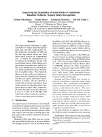
Figure 1: An acquired SCF for a verb “yield”
In their study, they first acquire fine-grained
SCFs using the unsupervised method proposed by
Briscoe and Carroll (1997) and Korhonen (2002).
Figure 1 shows an example of one acquired SCF
entry for a verb “yield.” Each SCF entry has
several fields about the observed SCF. I explain
here only its portion related to this study. The
TARGET field is a word stem, the first number in
the CLASSES field indicates an SCF type, and the

FREQCNT field shows how often words derivable
from the word stem appeared with the SCF type in
the training corpus. The obtained SCFs comprise
the total 163 SCF types which are originally based
on the SCFs in the ANLT (Boguraev and Briscoe,
1987) and COMLEX (Grishman et al., 1994) dic-
tionaries. In this example, the SCF type 24 corre-
sponds to an SCF of transitive verb.
They then obtain SCFs for the target lexicalized
grammar (the LinGO ERG (Copestake, 2002) in
their study) using a handcrafted translation map
from these 163 types to the SCF types in the target
grammar. They reported that they could achieve
a coverage improvement of 4.5% but that aver-
age parse time was doubled. This is because they
did not use any filtering method for the acquired
SCFs to suppress an increase of the lexical ambi-
guity. We definitely need some method to control
the quality of the acquired SCFs.
Their method is extendable to any lexicalized
grammars, if we could have a translation map from
these 163 types to the SCF types in the grammar.
2.2 Clustering of Verb SCF Distributions
There is some related work on clustering of
verbs according to their SCF probability distri-
butions (Schulte im Walde and Brew, 2002; Ko-
rhonen et al., 2003). Schulte im Walde and
(true) probability distribution
0
0.1

0.2
0.3
0.4
0.5
0.6
0.7
0.8
0.9
1
NP None NP_to-PP NP_PP PP
subcategorization frame
probability
apply
recognitio
n
threshold
Figure 2: SCF probability distributions for apply
Brew (2002) used the k-Means (Forgy, 1965) al-
gorithm to cluster SCF distributions for monose-
mous verbs while Korhonen et al. (2003) applied
other clustering methods to cluster polysemic SCF
data. These studies aim at obtaining verb seman-
tic classes, which are closely related to syntactic
behavior of argument selection (Levin, 1993).
Korhonen (2002) made use of SCF distributions
for representative verbs in Levin’s verb classes to
obtain accurate back-off estimates for all the verbs
in the classes. In this study, I assume that there
are classes whose element words have identical
SCF types. I then obtain these classes by clus-

tering acquired SCFs, using information available
in the target lexicon, and directly use the obtained
classes to eliminate implausible SCFs.
3 Method
3.1 Estimation of Confidence Values for SCFs
I first create an SCF confidence-value vector v
i
for
each word w
i
, an object for clustering. Each el-
ement v
ij
in v
i
represents a confidence value of
SCF s
j
for a word w
i
, which expresses how strong
the evidence is that the word w
i
has SCF s
j
. Note
that a confidence value conf
ij
is not a probability
that a word w

i
appears with SCF s
j
but a proba-
bility of existence of SCF s
j
for the word w
i
.In
this study, I assume that a word w
i
appears with
each SCF s
j
with a certain (non-zero) probabil-
ity
θ
ij
(= p(s
ij
|w
i
) > 0 where
∑
j
θ
ij
= 1), but only
SCFs whose probabilities exceed a certain thresh-
old are recognized in the lexicon. I hereafter call

this threshold recognition threshold. Figure 2 de-
picts a probability distribution of SCF for apply.
In this context, I can regard a confidence value of
each SCF as a probability that the probability of
that SCF exceeds the recognition threshold.
One intuitive way to estimate a confidence value
is to assume an observed probability, i.e., relative
frequency, is equal to a probability
θ
ij
of SCF s
j
for a word w
i
(
θ
ij
= freq
ij
/
∑
j
freq
ij
where freq
ij
is a frequency that a word w
i
appears with SCF s
j

in corpora). When the relative frequency of s
j
for
a word w
i
exceeds the recognition threshold, its
confidence value conf
ij
is set to 1, and otherwise
conf
ij
is set to 0. However, an observed probabil-
ity is unreliable for infrequent words. Moreover,
when we want to encode confidence values of re-
liable SCFs in the target grammar, we cannot dis-
tinguish the confidence values of those SCFs with
confidence values of acquired SCFs.
The other promising way to estimate a confi-
dence value, which I adopt in this study, is to as-
sume a probability
θ
ij
as a stochastic variable in
the context of Bayesian statistics (Gelman et al.,
1995). In this context, a posteriori distribution of
the probability
θ
ij
of an SCF s
j

for a word w
i
is
given by:
p(
θ
ij
|D)=
P(
θ
ij
)P(D|
θ
ij
)
P(D)
=
P(
θ
ij
)P(D|
θ
ij
)

1
0
P(
θ
ij

)P(D|
θ
ij
)d
θ
ij
, (1)
where P(
θ
ij
) is a priori distribution, and D is the
data we have observed. Since every occurrence
of SCFs in the data D is independent with each
other, the data D can be regarded as Bernoulli tri-
als. When we observe the data D that a word w
i
appears n times in total and x(≤ n) times with SCF
s
j
,
1
its conditional distribution is represented by
binominal distribution:
P(D|
θ
ij
)=

n
x


θ
x
ij
(1−
θ
ij
)
(n−x)
. (2)
To calculate this a posteriori distribution, I need
to define the a priori distribution P(
θ
ij
). The ques-
tion is which probability distribution of
θ
ij
can
appropriately reflects prior knowledge. In other
words, it should encode knowledge we use to es-
timate SCFs for unknown words. I simply deter-
mine it from distributions of observed probability
values of s
j
for words seen in corpora
2
by using
1
The values of FREQCNT is used to obtain n and x.

2
I estimated a priori distribution separately for each type
of SCF from words that appeared more than 50 times in the
training corpus in the following experiments.
a method described in (Tsuruoka and Chikayama,
2001). In their study, they assume a priori distri-
bution as the beta distribution defined as:
p(
θ
ij
|
α
,
β
)=
θ
α
−1
ij
(1−
θ
ij
)
β
−1
B(
α
,
β
)

, (3)
where B(
α
,
β
)=

1
0
θ
α
−1
ij
(1 −
θ
ij
)
β
−1
d
θ
ij
. The
value of
α
and
β
is determined by moment esti-
mation.
3

By substituting Equations 2 and 3 into
Equation 1, I finally obtain the a posteriori distri-
bution p(
θ
ij
|D) as:
p(
θ
ij
|
α
,
β
,D)=c·
θ
x+
α
−1
ij
(1−
θ
ij
)
n−x+
β
−1
,(4)
where c =

n

x

/(B(
α
,
β
)

1
0
P(
θ
ij
)P(D|
θ
ij
)d
θ
ij
).
When I regard the recognition threshold as t,I
can calculate a confidence value conf
ij
that a word
w
i
can have s
j
by integrating the a posteriori dis-
tribution p(

θ
ij
|D) from the threshold t to 1:
conf
ij
=

1
t
c·
θ
x+
α
−1
ij
(1−
θ
ij
)
n−x+
β
−1
d
θ
ij
.(5)
By using this confidence value, I represent an SCF
confidence-value vector v
i
for a word w

i
in the ac-
quired SCF lexicon (v
ij
= con f
ij
).
In order to combine SCF confidence-value vec-
tors for words acquired from corpora and those for
words in the lexicon of the target grammar, I also
represent an SCF confidence-value vector v

i
for a
word w

i
in the target grammar by:
v

ij
=

1−
ε
w

i
has s
j

in the lexicon
ε
otherwise,
(6)
where
ε
expresses an unreliability of the lexicon.
In this study, I trust the lexicon as much as possible
by setting
ε
to the machine epsilon.
3.2 Clustering of SCF Confidence-Value
Vectors
I next present a clustering algorithm of words
according to their SCF confidence-value vectors.
Given k initial representative vectors called cen-
troids, my algorithm iteratively updates clusters by
assigning each data object to its closest centroid
3
The expectation and variance of the beta distribution are
made equal to those of the observed probability values.
Input: a set of SCF confidence-value
vectors V = {v
1
,v
2
, ,v
n
}⊆R
m

a distance function d : R
m
× Z
m
→ R
a function to compute a centroid
µ
: {v
j
1
,v
j
2
, ,v
j
l
}→Z
m
initial centroids C = {c
1
,c
2
, ,c
k
}⊆Z
m
Output: a set of clusters {C
j
}
while cluster members are not stable do

foreach cluster C
j
C
j
= {v
i
|∀c
l
,d(v
i
,c
j
) ≥ d(v
i
,c
l
)} (1)
end foreach
foreach clusters C
j
c
j
=
µ
(C
j
) (2)
end foreach
end while
return {C

j
}
Figure 3: Clustering algorithm for SCF
confidence-value vectors
and recomputing centroids until cluster members
become stable, as depicted in Figure 3.
Although this algorithm is roughly based on the
k-Means algorithm, it is different from k-Means in
important respects. I assume the elements of the
centroids of the clusters as a discrete value of 0 or
1 because I want to obtain clusters whose element
words have the exactly same set of SCFs.
I then derive a distance function d to calculate
a probability that a data object v
i
should have an
SCF set represented by a centroid c
m
as follows:
d(v
i
,c
m
)=
∏
c
mj
=1
v
ij

·
∏
c
mj
=0
(1−v
ij
). (7)
By using this function, I can determine the closest
cluster as argmax
C
m
d(v
i
,c
m
) ((1) in Figure 3).
After every assignment, I calculate a next cen-
troid c
m
of each cluster C
m
((2) in Figure 3) by
comparing a probability that the words in the clus-
ter have an SCF s
j
and a probability that the words
in the cluster do not have the SCF s
j
as follows:

c
mj
=



1 when
∏
v
i
∈C
m
v
ij
>
∏
v
i
∈C
m
(1−v
ij
)
0 otherwise.
(8)
I next address the way to determine the num-
ber of clusters and initial centroids. In this study,
I assume that the most of the possible set of SCFs
for words are included in the lexicon of the tar-
get grammar,

4
and make use of the existing sets of
4
When the lexicon is less accurate, I can determine the
number of clusters using other algorithms (Hamerly, 2003).
SCFs for the words in the lexicon to determine the
number of clusters and initial centroids. I first ex-
tract SCF confidence-value vectors from the lexi-
con of the grammar. By eliminating duplications
from them and regarding
ε
= 0 in Equation 6, I ob-
tain initial centroids c
m
. I then initialize the num-
ber of clusters k to the number of c
m
.
I finally update the acquired SCFs using the ob-
tained clusters and the confidence values of SCFs
in this order. I call the following procedure cen-
troid cut-off t when the confidence values are es-
timated under the recognition threshold t. Since
the value c
mj
of a centroid c
m
in a cluster C
m
rep-

resents whether the words in the cluster can have
SCF s
j
, I first obtain SCFs by collecting SCF s
j
for a word w
i
∈ C
m
when c
mj
is 1. I then elimi-
nate implausible SCFs s
j
for w
i
from the resulting
SCFs according to their confidence values conf
ij
.
In the following, I compare centroid cut-off
with frequency cut-off and confidence cut-off t,
which use relative frequencies and confidence val-
ues calculated under the recognition threshold t,
respectively. Note that these cut-offs use only
corpus-based statistics to eliminate SCFs.
4 Experiments
I applied my method to SCFs acquired from
135,902 sentences of mobile phone newsgroup
postings archived by Google.com, which is the

same data used in (Carroll and Fang, 2004). The
number of acquired SCFs was 14,783 for 3,864
word stems, while the number of SCF types in
the data was 97. I then translated the 163 SCF
types into the SCF types of the XTAG English
grammar (XTAG Research Group, 2001) and the
LinGO ERG (Copestake, 2002)
5
using translation
mappings built by Ted Briscoe and Dan Flickinger
from 23 of the SCF types into 13 (out of 57 possi-
ble) XTAG SCF types, and 129 into 54 (out of 216
possible) ERG SCF types.
To evaluate my method, I split each lexicon of
the two grammars into the training SCFs and the
testing SCFs. The words in the testing SCFs were
included in the acquired SCFs. When I apply
my method to the acquired SCFs using the train-
ing SCFs and evaluate the resulting SCFs with the
5
I used the same version of the LinGO ERG as (Carroll
and Fang, 2004) (1.4; April 2003) but the map is updated.
0
0.2
0.4
0.6
0.8
1
0 0.2 0.4 0.6 0.8 1
Recall

Precision
A
B C D
A: frequency cut-off
B: confidence cut-off 0.01
C: confidence cut-off 0.03
D: confidence cut-off 0.05
0
0.2
0.4
0.6
0.8
1
0 0.2 0.4 0.6 0.8 1
Recall
Precision
A
B
C
D
A: frequency cut-off
B: confidence cut-off 0.01
C: confidence cut-off 0.03
D: confidence cut-off 0.05
XTAG ERG
Figure 4: Precision and recall of the resulting SCFs using confidence cut-offs and frequency cut-off: the
XTAG English grammar (left) the LinGO ERG (right)
0
0.2
0.4

0.6
0.8
1
0 0.2 0.4 0.6 0.8 1
Recall
Precision
A
B
C
D
A: frequency cut-off
B: centroid cut-off* 0.05
C: centroid cut-off 0.05
D: confidence cut-off 0.05
0
0.2
0.4
0.6
0.8
1
0 0.2 0.4 0.6 0.8 1
Recall
Precision
A
B
C
D
A: frequency cut-off
B: centroid cut-off* 0.05
C: centroid cut-off 0.05

D: confidence cut-off 0.05
XTAG ERG
Figure 5: Precision and recall of the resulting SCFs using confidence cut-off and centroid cut-off: the
XTAG English grammar (left) the LinGO ERG (right)
testing SCFs, we can estimate to what extent my
method can preserve reliable SCFs for words un-
known to the grammar.
6
The XTAG lexicon was
split into 9,437 SCFs for 8,399 word stems as
training and 423 SCFs for 280 word stems as test-
ing, while the ERG lexicon was split into 1,608
SCFs for 1,062 word stems as training and 292
SCFs for 179 word stems as testing. I extracted
SCF confidence-value vectors from the training
SCFs and the acquired SCFs for the words in the
testing SCFs. The number of the resulting data
objects was 8,679 for XTAG and 1,241 for ERG.
The number of initial centroids
7
extracted from
the training SCFs was 49 for XTAG and 53 for
ERG. I then performed clustering of 8,679 data
objects into 49 clusters and 1,241 data objects into
6
I here assume that the existing SCFs for the words in the
lexicon is more reliable than the other SCFs for those words.
7
I used the vectors that appeared for more than one word.
53 clusters, and then evaluated the resulting SCFs

by comparing them to the testing SCFs.
I first compare confidence cut-off with fre-
quency cut-off to observe the effects of Bayesian
estimation. Figure 4 shows precision and recall
of the SCFs obtained using frequency cut-off and
confidence cut-off 0.01, 0.03, and 0.05 by varying
threshold for the confidence values and the relative
frequencies from 0 to 1.
8
The graph indicates that
the confidence cut-offs achieved higher recall than
the frequency cut-off, thanks to the a priori distri-
butions. When we compare the three confidence
cut-offs, we can improve precision using higher
recognition thresholds while we can improve re-
call using lower recognition thresholds. This is
quite consistent with our expectations.
8
Precision=
Correct SCFs for the words in the resulting SCFs
All SCFs for the words in the resulting SCFs
Recall =
Correct SCFs for the words in the resulting SCFs
All SCFs for the words in the test SCFs
I then compare centroid cut-off with confidence
cut-off to observe the effects of clustering. Fig-
ure 5 shows precision and recall of the resulting
SCFs using centroid cut-off 0.05 and the confi-
dence cut-off 0.05 by varying the threshold for the
confidence values. In order to show the effects

of the use of the training SCFs, I also performed
clustering of SCF confidence-value vectors in the
acquired SCFs with random initialization (k =49
(for XTAG) and 53 (for ERG); centroid cut-off
0.05*). The graph shows that clustering is mean-
ingful only when we make use of the reliable SCFs
in the manually-coded lexicon. The centroid cut-
off using the lexicon of the grammar boosted pre-
cision compared to the confidence cut-off.
The difference between the effects of my
method on XTAG and ERG would be due to the
finer-grained SCF types of ERG. This resulted
in lower precision of the acquired SCFs for ERG,
which prevented us from distinguishing infrequent
(correct) SCFs from SCFs acquired in error. How-
ever, since unusual SCFs tend to be included in the
lexicon, we will be able to have accurate clusters
for unknown words with smaller SCF variations as
we achieved in the experiments with XTAG.
5 Concluding Remarks and Future Work
In this paper, I presented a method to improve
the quality of SCFs acquired from corpora using
existing lexicon resources. I applied my method
to SCFs acquired from corpora using lexicons of
the XTAG English grammar and the LinGO ERG,
and have shown that it can eliminate implausible
SCFs, preserving more reliable SCFs.
In the future, I need to evaluate the quality of
the resulting SCFs by manual analysis and by us-
ing the extended lexicons to improve parsing. I

will investigate other clustering methods such as
hierarchical clustering, and use other information
for clustering such as semantic preference of argu-
ments of SCFs to have more accurate clusters.
Acknowledgments
I thank Yoshimasa Tsuruoka and Takuya Mat-
suzaki for their advice on probabilistic modeling,
Alex Fang for his help in using the acquired SCFs,
and Anna Korhonen for her insightful suggestions
on evaluation. I am also grateful to Jun’ichi Tsujii,
Yusuke Miyao, John Carroll and the anonymous
reviewers for their valuable comments. This work
was supported in part by JSPS Research Fellow-
ships for Young Scientists and in part by CREST,
JST (Japan Science and Technology Agency).
References
B. Boguraev and T. Briscoe. 1987. Large lexicons for natural
language processing: utilising the grammar coding system
of LDOCE. Computational Linguistics, 13(4):203–218.
T. Briscoe and J. Carroll. 1997. Automatic extraction of
subcategorization from corpora. In Proc. the fifth ANLP,
pages 356–363.
J. Carroll and A. C. Fang. 2004. The automatic acquisition
of verb subcategorizations and their impact on the perfor-
mance of an HPSG parser. In Proc. the first ijc-NLP, pages
107–114.
A. Copestake. 2002. Implementing typed feature structure
grammars. CSLI publications.
E. W. Forgy. 1965. Cluster analysis of multivariate data: Ef-
ficiency vs. interpretability of classifications. Biometrics,

21:768–780.
A. Gelman, J. B. Carlin, H. S. Stern, and D. B. Rubin, editors.
1995. Bayesian Data Analysis. Chapman and Hall.
R. Grishman, C. Macleod, and A. Meyers. 1994. Comlex
syntax: Building a computational lexicon. In Proc. the
15th COLING, pages 268–272.
G. Hamerly. 2003. Learning structure and concepts in data
through data clustering. Ph.D. thesis, University of Cali-
fornia, San Diego.
A. Korhonen, Y. Krymolowski, and Z. Marx. 2003. Clus-
tering polysemic subcategorization frame distributions se-
mantically. In Proc. the 41st ACL, pages 64–71.
A. Korhonen. 2002. Subcategorization Acquisition. Ph.D.
thesis, University of Cambridge.
B. Levin. 1993. English Verb Classes and Alternations.
Chicago University Press.
A. Sarkar, F. Xia, and A. K. Joshi. 2000. Some experiments
on indicators of parsing complexity for lexicalized gram-
mars. In Proc. the 18th COLING workshop, pages 37–42.
S. Schulte im Walde and C. Brew. 2002. Inducing German
semantic verb classes from purely syntactic subcategorisa-
tion information. In Proc. the 41st ACL, pages 223–230.
Y. Tsuruoka and T. Chikayama. 2001. Estimating reliability
of contextual evidences in decision-list classifiers under
Bayesian learning. In Proc. the sixth NLPRS, pages 701–
707.
XTAG Research Group. 2001. A Lexicalized Tree Adjoin-
ing Grammar for English. Technical Report IRCS-01-03,
IRCS, University of Pennsylvania.