Báo cáo khoa học: "Active Learning for Statistical Natural Language Parsing" potx

Active Learning for Statistical Natural Language Parsing
Min Tang
Spoken Language Systems Group
MIT Laboratory for Computer Science
Cambridge, Massachusetts 02139, USA

Xiaoqiang Luo Salim Roukos
IBM T.J. Watson Research Center
Yorktown Heights, NY 10598
xiaoluo,
Abstract
It is necessary to have a (large) annotated cor-
pus to build a statistical parser. Acquisition of
such a corpus is costly and time-consuming.
This paper presents a method to reduce this
demand using active learning, which selects
what samples to annotate, instead of annotating
blindly the whole training corpus.
Sample selection for annotation is based upon
“representativeness” and “usefulness”. A
model-based distance is proposed to measure
the difference of two sentences and their most
likely parse trees. Based on this distance, the
active learning process analyzes the sample dis-
tribution by clustering and calculates the den-
sity of each sample to quantify its representa-
tiveness. Further more, a sentence is deemed as
useful if the existing model is highly uncertain
about its parses, where uncertainty is measured
by various entropy-based scores.
Experiments are carried out in the shallow se-

mantic parser of an air travel dialog system.
Our result shows that for about the same pars-
ing accuracy, we only need to annotate a third
of the samples as compared to the usual random
selection method.
1 Introduction
A prerequisite for building statistical parsers (Jelinek et
al., 1994; Collins, 1996; Ratnaparkhi, 1997; Charniak,
1997) is the availability of a (large) corpus of parsed sen-
tences. Acquiring such a corpus is expensive and time-
consuming and is often the bottleneck to build a parser
for a new application or domain. The goal of this study is
to reduce the amount of annotated sentences (and hence
the development time) required for a statistical parser to
achieve a satisfactory performance using active learning.
Active learning has been studied in the context of many
natural language processing (NLP) applications such as
information extraction(Thompson et al., 1999), text clas-
sification(McCallum and Nigam, 1998) and natural lan-
guage parsing(Thompson et al., 1999; Hwa, 2000), to
name a few. The basic idea is to couple tightly knowl-
edge acquisition, e.g., annotating sentences for parsing,
with model-training, as opposed to treating them sepa-
rately. In our setup, we assume that a small amount of
annotated sentences is initially available, which is used
to build a statistical parser. We also assume that there is
a large corpus of unannotated sentences at our disposal –
this corpus is called active training set. A batch of sam-
ples
1

is selected using algorithms developed here, and are
annotated by human beings and are then added to training
data to rebuild the model. The procedure is iterated until
the model reaches a certain accuracy level.
Our efforts are devoted to two aspects: first, we be-
lieve that the selected samples should reflect the underly-
ing distribution of the training corpus. In other words, the
selected samples need to be representative. To this end,
a model-based structural distance is defined to quantify
how “far” two sentences are apart, and with the help of
this distance, the active training set is clustered so that
we can define and compute the “density” of a sample;
second, we propose and test several entropy-based mea-
sures to quantify the uncertainty of a sample in the active
training set using an existing model, as it makes sense
to ask human beings to annotate the portion of data for
which the existing model is not doing well. Samples are
selected from the clusters based on uncertainty scores.
The rest of the paper is organized as follows. In Sec-
tion 2, a structural distance is first defined based on the se-
quential representation of a parse tree. It is then straight-
forward to employ a k-means algorithm to cluster sen-
tences in the active training set. Section 3 is devoted to
confidence measures, where three uncertainty measures
are proposed. Active learning results on the shallow se-
mantic parser of an air travel dialog system are presented
1
A sample means a sentence in this paper.
Computational Linguistics (ACL), Philadelphia, July 2002, pp. 120-127.
Proceedings of the 40th Annual Meeting of the Association for

in Section 4. A summary of related work is given in
Section 5. The paper closes with conclusions and future
work.
2 Sentence Distance and Clustering
To characterize the “representativeness” of a sentence, we
need to know how far two sentences are apart so that we
can measure roughly how many similar sentences there
are in the active training set. For our purpose, the dis-
tance ought to have the property that two sentences with
similar structures have a small distance, even if they are
lexically different. This leads us to define the distance be-
tween two sentences based on their parse trees, which are
obtained by applying an existing model to the active train-
ing set. However, computing the distance of two parse
trees requires a digression of how they are represented in
our parser.
2.1 Event Representation of Parse Trees
A statistical parser computes , the probability of a
parse given a sentence . Since the space of the entire
parses is too large and cannot be modeled directly, a parse
tree is decomposed as a series of individual actions
. In the parser (Jelinek et al., 1994) we
used in this study, this is accomplished through a bottom-
up-left-most (BULM) derivation. In the BULM deriva-
tion, there are three types of parse actions: tag, label and
extension. There is a corresponding vocabulary for tag
or label, and there are four extension directions: RIGHT,
LEFT, UP and UNIQUE. If a child node is the only node
under a label, the child node is said to extend UNIQUE
to its parent node; if there are multiple children under a

parent node, the left-most child is said to extend RIGHT
to the parent node, the right-most child node is said to
extend LEFT to the parent node, while all the other in-
termediate children are said to extend UP to their parent
node. The BULM derivation can be best explained by an
example in Figure 1.
1
3
5
7
11
13
(12)
(16)
(9) (15)
(2)
(4)
(17)
(10)
(14)(6)
(8)
wd
wd
city
wd citycity
LOC
LOC
S
fly from new
boston

york to
Figure 1: Serial decomposition of a parse tree
as 17 parsing actions: tags (1,3,5,7,11,13) – blue
boxes, labels (9,15,17)–green underlines, extensions
(2,4,6,8,10,12,14,16)– red parentheses. Numbers indi-
cate the order of actions.
The input sentence is fly from new york to
boston. Numbers on its semantic parse tree indicate
the order of parse actions while colors indicate types of
actions: tags are numbered in blue boxes, extensions in
red parentheses and labels in green underlines. For this
example, the first action is tagging the first word fly
given the sentence; the second action is extending the tag
wd RIGHT, as the tag wd is the left-most child of the con-
stituent S; and the third action is tagging the second word
from given the sentence and the two proceeding actions,
and so on and so forth.
We define an event as a parse action together with its
context. It is clear that the BULM derivation converts a
parse tree into a unique sequence of parse events, and a
valid event sequence corresponds to a unique parse tree.
Therefore a parse tree can be equivalently represented by
a sequence of events. Let be the set of tagging ac-
tions, be the labeling actions and be the ex-
tending actions of , and let be the sequence of ac-
tions ahead of the action , then can be rewritten
as:
(1)
Note that . The three
models (1) can be trained using decision trees (Jelinek et

al., 1994; Breiman et al., 1984).
Note that raw context space is too huge to
store and manipulate efficiently. In our implementation,
contexts are internally represented as bitstrings through a
set of pre-designed questions. Answers of each question
are represented as bitstrings. To support questions like
“what is the previous word (or tag, label, extension)?”,
word, tag, label and extension vocabularies are all en-
coded as bitstrings. Words are encoded through an au-
tomatic clustering algorithm (Brown et al., 1992) while
tags, labels and extensions are normally encoded using
diagonal bits. An example can be found in (Luo et al.,
2002).
In summary, a parse tree can be represented uniquely
by a sequence of events, while each event can in turn be
represented as a bitstring. With this in mind, we are now
ready to define a structural distance for two sentences
given an existing model.
2.2 Sentence Distance
Recall that it is assumed that there is a statistical parser
trained with a small amount of annotated data. To
infer structures of two sentences and , we use
to decode and and get their most likely parse trees
and . The distance between and , given ,
is defined as the distance between and ,
or:
(2)
To emphasize the dependency on , we denote the dis-
tance as . Note that we assume here that
and have similar “true” parses if they have similar

structures under the current model .
We have shown in Section 2.1 that a parse tree can
be represented by a sequence of events, each of which
can in turn be represented as bitstrings through answer-
ing questions. Let be the
sequence representation for ( ), where
, and is the context and is the
parsing action of the event of the parse tree . We
can define the distance between two sentences as
(3)
The distance between two sequences and is com-
puted as the editing distance using dynamic program-
ming (Rabiner and Juang, 1993). We now describe the
distance between two individual events.
We take advantage of the fact that contexts can
be encoded as bitstrings, and define the distance between
two contexts as the Hamming distance between their bit-
string representations. We further define the distance be-
tween two parsing actions as follows: it is either or a
constant if two parse actions are of the same type (re-
call there are three types of parsing actions: tag, label and
extension), and infinity if different types. We choose to
be the number of bits in to emphasize the importance
of parsing actions in distance computation. Formally, let
be the type of action , then
(4)
where is the Hamming distance, and
if
if Y( ) = Y( )
if Y( Y( ).

(5)
Computing the editing distance (3) requires dynamic
programming and it is computationally extensive. To
speed up computation, we can choose to ignore the dif-
ference in contexts, or in other words, (4) becomes
(6)
The distance makes it possible to characterize
how dense a sentence is. Given a set of sentences
, the density of sample is defined as:
(7)
That is, the sample density is defined as the inverse of
its average distance to other samples. We also define the
centroid
2
of S as
argmax (8)
2.3 K-Means Clustering
With the model-based distance measure defined above,
we can use the K-means algorithm to cluster sentences.
A sketch of the algorithm (Jelinek, 1997) is as follows.
Let be the set of sentences to be
clustered.
1. Initialization. Partition into k ini-
tial clusters ( ). Let .
2. Find the centroid for each collection , that is:
argmin
3. Re-partition into clusters
, where
4. Let . Repeat Step 2 and Step 3 untill the al-
gorithm converges (e.g., relative change of the total

distortion is smaller than a threshold).
For each iteration we need to compute:
the distance between samples and cluster centers
,
the pair-wise distances within each cluster.
The basic operation here is to compute the distance be-
tween two sentences, which involves a dynamic program-
ming process and is time-consuming. The complexity of
this algorithm is, if we assume the N samples are uni-
formly distributed between the k clusters, approximately
, or when . In our experi-
ments and , we need to call the
dynamic programming routine times each itera-
tion!
2
We constrain the centroid to be an element of the set as it
is not clear how to “average” sentences.
To speed up, dynamic programming is constrained so
that only the band surrounding the diagonal line (Rabiner
and Juang, 1993) is allowed, and repeated sentences are
stored as a unique copy with its count so that computation
for the same sentence pair is never repeated. The latter is
a quite effective for dialog systems as a sentence is often
seen more than once in the training corpus.
3 Uncertainty Measures
Intuitively, we would like to select samples that the cur-
rent model is not doing well. The current model’s un-
certainty about a sentence could be because similar sen-
tences are under-represented in the (annotated) training
set, or similar sentences are intrinsically difficult. We

take advantage of the availability of parsing scores from
the existing statistical parser and propose three entropy-
based uncertainty scores.
3.1 Change of Entropy
After decision trees are grown, we can compute the en-
tropy of each leaf node as:
(10)
where sums over either tag, label or extension vocab-
ulary, and is simply , where is the
count of in leaf node . The model entropy is the
weighted sum of :
(11)
where . Note that is the log proba-
bility of training events.
After seeing an unlabeled sentence , we can decode it
using the existing model and get its most probable parse
. The tree can then be represented by a sequence of
events, which can be “poured” down the grown trees, and
the count can be updated accordingly – denote the
updated count as . A new model entropy can be
computed based on , and the absolute difference,
after it is normalized by the number of events in , is
the change of entropy we are after:
(12)
It is worth pointing out that is a “local” quantity in
that the vast majority of is equal to , and thus
we only have to visit leaf nodes where counts change. In
other words, can be computed efficiently.
characterizes how a sentence “surprises” the ex-
isting model: if the addition of events due to changes a

lot of , and consequently, , the sentence is proba-
bly not well represented in the initial training set and
will be large. We would like to annotate these sentences.
3.2 Sentence Entropy
Now let us consider another measurement which seeks to
address the intrinsic difficulty of a sentence. Intuitively,
we can consider a sentence more difficult if there are po-
tentially more parses. We calculate the entropy of the dis-
tribution over all candidate parses as the sentence entropy
to measure the intrinsic ambiguity.
Given a sentence , the existing model could gener-
ate the top most likely parses ,
each having a probability :
(13)
where is the possible parse and is its associated
score. Without confusion, we drop ’s dependency on
and define the sentence entropy as:
(14)
where:
(15)
3.3 Word Entropy
As we can imagine, a long sentence tends to have more
possible parsing results not because it is difficult but sim-
ply because it is long. To counter this effect, we can nor-
malize the sentence entropy by the length of sentence to
calculate per word entropy of a sentence:
(16)
where is the number of words in .
20 40 60 80 100 120
0

0.02
0.04
0.06
0.08
0.1
0.12
0.14
Sentence Length
Average Change of Entropy H∆
20 40 60 80 100 120
0
0.02
0.04
0.06
0.08
0.1
0.12
Sentence Length
Average Word Entropy Hw
20 40 60 80 100 120
0
0.5
1
1.5
2
2.5
3
3.5
4
Sentence Length

Average Sentence Entropy Hs
Figure 2: Histograms of 3 uncertainty scores vs. sentence
lengths
Figure 2 illustrates the distribution of the three differ-
ent uncertainty scores versus sentence lengths. favors
longer sentences more. This can be explained as follows:
longer sentences tend to have more complex structures
( extension and labeling ) than shorter sentences. And
the models for these complex structures are relatively less
trained as compared with models for tagging. As a result,
longer sentences would have higher change of entropy, in
other words, larger impact on models.
As explained above, longer sentences also have larger
sentence entropy. After normalizing, this trend is re-
versed in word entropy.
4 Experimental Results and Analysis
All experiments are done with a shallow semantic parser
(a.k.a. classer (Davies et al, 1999)) of the natural
language understanding part in DARPA Communica-
tor (DARPA Communicator Website, 2000). We built an
initial model using 1000 sentences. We have 20951 un-
labeled sentences for the active learner to select samples.
An independent test set consists of 4254 sentences. A
fixed batch size is used through out our experi-
ments.
Exact match is used to compute the accuracy, i.e.,
the accuracy is the number of sentences whose decod-
ing trees are exactly the same as human annotation di-
vided by the number of sentences in the test set. The ef-
fectiveness of active learning is measured by comparing

learning curves (i.e., test accuracy vs. number of training
sentences ) of active learning and random selection.
4.1 Sample Selection Schemes
We experimented two basic sample selection algorithms.
The first one is selecting samples based solely on uncer-
tainty scores, while the second one clusters sentences,
and then selects the most uncertain ones from each clus-
ter.
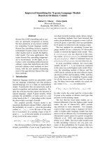
Uncertainty Only: at each active learning iteration,
the most uncertain sentences are selected.
The drawback of this selection method is that it risks
selecting outliers because outliers are likely to get
high uncertainty scores under the existing models.
Figure 3 shows the test accuracy of this selection
method against the number of samples selected from
the active training set.
Short sentences tends to have higher value of
while sentence-based uncertainty scores (in terms of
or ) are low. Since we use the sentences as
the basic units, it is not surprising that -based
method performs poorly while the other two perform
very well.
Most Uncertain Per Cluster: In our implemen-
tation, we cluster the active training set so that
100 200 300 400 500 600 700 800 900 1000
60
65
70
75
80

85
90
Sample Selection By Confidence Only
Number of Sentences Selected
Accuracy(%)
Random Selection
H∆: Change Entropy
Hw: Word Entropy
Hs: Sentence Entropy
Figure 3: Learning curves using uncertainty score only:
pick samples with highest entropies
the number of clusters equals the batch size. This
scheme selects the sentence with the highest uncer-
tain score from each cluster.
We expect that restricting sample selection to each
cluster would fix the problem that tends to be
large for short sentences, as short sentences are
likely to be in one cluster and long sentences will get
a fair chance to be selected in other clusters. This is
verified by the learning curves in Figure 4. Indeed,
performs as well as most of the time. And all
active learning algorithms perform better than ran-
dom selection.
100 200 300 400 500 600 700 800 900 1000
60
65
70
75
80
85

90
Accuracy of Sample Selection(No Weighting)
Number of Sentences Selected
Accuracy(%)
Random Selection
H∆: Change Entropy
Hw: Word Entropy
Hs: Sentence Entropy
Figure 4: Learning curves of selecting the most uncertain
sample from each cluster.
4.2 Weighting Samples
In the sample selection process we calculated the density
of each sample. For those samples selected, we also have
the knowledge of their correct annotations, which can
be used to evalutate the model’s performance on them.
We exploit this knowledge and experiment two weight-
ing schemes.
Weight by Density:
A sample with higher density should be assigned
greater weights because the model can benefit
more by learning from this sample as it has more
neighbors. We calculate the density of a sample
inside its cluster so we need to adjust the density by
cluster size to avoid the unwanted bias toward small
clusters. For cluster
, the weight for
sample is proportional to .
Weight by Performance: The idea of weight by
performance is to focus the model on its weakness
when it knows about it. The model can test itself on

its training set where the truth is known and assign
greater weights to sentences it parses incorrectly.
In our experiment, weights are updated as follows:
the initial weight for a sentence is its count; and if
the human annotation of a selected sentence differs
from the current model output, its weight is multi-
plied by . We did not experiment more compli-
cated weighting scheme (like AdaBoost) since we
only want to see if weighting has any effect on ac-
tive learning result.
Figure 5 and Figure 6 are learning curves when se-
lected samples are weighted by density and performance,
which are described in Section 4.2.
100 200 300 400 500 600 700 800 900 1000
60
65
70
75
80
85
90
Accuracy of Sample Selection(Weighted by Density)
Number of Sentences Selected
Accuracy(%)
Random Selection
H∆: Change Entropy
Hw: Word Entropy
Hs: Sentence Entropy
Figure 5: Active learning curve: selected sentences are
weighted by density

The effect of weighting samples is highlighted in Ta-
ble 1, where results are obtained after 1000 samples are
selected using the same uncertainty score , but with
different weighting schemes. Weighting samples by den-
sity leads to the best performance. Since weighting sam-
ples by density is a way to tweak sample distribution of
100 200 300 400 500 600 700 800 900 1000
60
65
70
75
80
85
90
Accuracy of Sample Selection(Weighted by Performance)
Number of Sentences Selected
Accuracy(%)
Random Selection
H∆: Change Entropy
Hw: Word Entropy
Hs: Sentence Entropy
Figure 6: Active learning curve: selected sentences are
weighted based on performance
training set toward the distribution of the entire sample
space, including unannotated sentences, it indicates that
it is important to ensure the distribution of training set
matches that of the sample space. Therefore, we believe
that clustering is a necessary and useful step.
Table 1: Weighting effect
Weighting none density performance

Test Accuracy(%) 79.8 84.3 80.7
4.3 Effect of Clustering
Figure 7 compares the best learning curve using only un-
certainty score(i.e., sentence entropy in Figure 3) to select
samples with the best learning curve resulted from clus-
tering and the word entropy . It is clear that clustering
results in a better learning curve.
4.4 Summary Result
Figure 8 shows the best active learning result compared
with that of random selection. The learning curve for ac-
tive learning is obtained using as uncertainty measure
and selected samples are weighted by density. Both ac-
tive learning and random selection are run 40 times, each
time selecting 100 samples. The horizontal line on the
graph is the performance if all 20K sentences are used. It
is remarkable to notice that active learning can use far less
samples ( usually less than one third ) to achieve the same
level of performance of random selection. And after only
about 2800 sentences are selected, the active learning re-
sult becomes very close to the best possible accuracy.
5 Previous Work
While active learning has been studied extensively in the
context of machine learning (Cohn et al., 1996; Freund
500 1000 1500 2000 2500
60
65
70
75
80
85

90
Effect of Clustering
Number of Sentences Selected
Accuracy(%)
Word Entropy(Hw)
Use sentence entropy only
Figure 7: Effect of clustering: entropy-based learning
curve (in plus) vs. sample selection with clustering and
uncertainty score(in triangle).
500 1000 1500 2000 2500 3000 3500 4000
60
65
70
75
80
85
90
Active Learning vs. Random Selection
Number of Sentences Selected
Accuracy(%)
Word Entropy(Hw), weighted by density
Random Selection
Use 20k Samples
Figure 8: Active learner uses one-third (about 1300 sen-
tences) of training data to achieve similar performance to
random selection (about 4000 sentence).
et al., 1997), and has been applied to text classifica-
tion (McCallum and Nigam, 1998) and part-of-speech
tagging (Dagan and Engelson, 1995), there are only a
handful studies on natural language parsing (Thompson

et al., 1999) and (Hwa, 2000; Hwa, 2001). (Thompson
et al., 1999) uses active learning to acquire a shift-reduce
parser, and the uncertainty of an unparseable sentence is
defined as the number of operators applied successfully
divided by the number of words. It is more natural to de-
fine uncertainty scores in our study because of the avail-
bility of parse scores. (Hwa, 2000; Hwa, 2001) is related
closely to our work in that both use entropy-based un-
certainty scores, but Hwa does not characterize the dis-
tribution of sample space. Knowing the distribution of
sample space is important since uncertainty measure, if
used alone for sample selection, will be likely to select
outliers. (Stolcke, 1998) used an entropy-based criterion
to reduce the size of backoff n-gram language models.
The major contribution of this paper is that a model-
based distance measure is proposed and used in active
learning. The distance measures structural difference of
two sentences relative to an existing model. Similar idea
is also exploited in (McCallum and Nigam, 1998) where
authors use the divergence between the unigram word
distributions of two documents to measure their differ-
ence. This distance enables us to cluster the active train-
ing set and a sample is then selected and weighted based
on both its uncertainty score and its density. (Sarkar,
2001) applied co-training to statistical parsing, where two
component models are trained and the most confident
parsing outputs of the existing model are incorporated
into the next training. This is a different venue for reduc-
ing annotation work in that the current model output is
directly used and no human annotation is assumed. (Luo

et al., 1999; Luo, 2000) also aimed to making use of unla-
beled data to improve statistical parsers by transforming
model parameters.
6 Conclusions and Future Work
We have examined three entropy-based uncertainty
scores to measure the “usefulness” of a sample to im-
proving a statistical model. We also define a distance for
sentences of natural languages. Based on this distance,
we are able to quantify concepts such as sentence density
and homogeneity of a corpus. Sentence clustering algo-
rithms are also developed with the help of these concepts.
Armed with uncertainty scores and sentence clusters, we
have developed sample selection algorithms which has
achieved significant savings in terms of labeling cost: we
have shown that we can use one-third of training data of
random selection and reach the same level of parsing ac-
curacy.
While we have shown the importance of both con-
fidence score and modeling the distribution of sample
space, it is not clear whether or not it is the best way to
combine or reconcile the two. It would be nice to have a
single number to rank candidate sentences. We also want
to test the algorithms developed here on other domains
(e.g., Wall Street Journal corpus). Improving speed of
sentence clustering is also worthwhile.
7 Acknowledgments
We thank Kishore Papineni and Todd Ward for many use-
ful discussions. The anonymous reviewer’s suggestions
to improve the paper is greatly appreciated. This work is
partially supported by DARPA under SPAWAR contract

number N66001-99-2-8916.
References
Leo Breiman, Jerome H. Friedman, Richard A. Olshen,
and Charles J. Stone. 1984. Classfication And Regres-
sion Trees. Wadsworth Inc.
P.F Brown, V.J.Della Pietra, P.V. deSouza, J.C Lai, and
R.L. Mercer. 1992. Class-based n-gram models of
natural language. Computational Linguistics, 18:467–
480.
E. Charniak. 1997. Statistical parsing with context-free
grammar and word statistics. In Proceedings of the
14th National Conference on Artificial Intelligence.
David A. Cohn, Zoubin Ghahramani, and Michael I. Jor-
dan. 1996. Active learning with statistical models. J.
of Artificial Intelligence Research, 4:129–145.
Michael Collins. 1996. A new statistical parser based on
bigram lexical dependencies. In Proc. Annual Meet-
ing of the Association for Computational Linguistics,
pages 184–191.
I. Dagan and S. Engelson. 1995. Committee-based sam-
pling for training probabilistic classifiers. In ICML.
DARPA Communicator Website. 2000.
.
K. Davies et al. 1999. The IBM conversational tele-
phony system for financial applications. In Proc. of
EuroSpeech, volume I, pages 275–278.
Yoav Freund, H. Sebastian Seung, Eli Shamir, and Naf-
tali Tishby. 1997. Selective sampling using query by
committee algorithm. Machine Leanring, 28:133–168.
Rebecca Hwa. 2000. Sample selection for statistical

grammar induction. In Proc.
EMNLP/VLC, pages
45–52.
Rebecca Hwa. 2001. On minimizing training corpus for
parser acquisition. In Proc. Computational Natu-
ral Language Learning Workshop. Morgan Kaufmann,
San Francisco, CA.
F. Jelinek, J. Lafferty, D. Magerman, R. Mercer, A. Rat-
naparkhi, and S. Roukos. 1994. Decision tree parsing
using a hidden derivation model. In Proc. Human Lan-
guage Technology Workshop, pages 272–277.
Frederick Jelinek. 1997. Statistical Methods for Speech
Recognition. MIT Press.
X. Luo, S. Roukos, and T. Ward. 1999. Unsupervised
adaptation of statistical parsers based on Markov trans-
form. In Proc. IEEE Workshop on Automatic Speech
Recognition and Understanding.
Xiaoqiang Luo, Salim Roukos, and Min Tang. 2002. Ac-
tive learning for statistical parsing. Technical report,
IBM Research Report.
X. Luo. 2000. Parser adaptation via Householder trans-
form. In Proc. ICASSP.
Andrew McCallum and Kamal Nigam. 1998. Employ-
ing EM and pool-based active learning for text clas-
sification. In Machine Learning: Proceedings of the
Fifteenth International Conference (ICML ’98), pages
359–367.
L. R. Rabiner and B. H. Juang. 1993. Fundamentals of
Speech Recognition. Prentice-Hall, Englewood Cliffs,
NJ.

Adwait Ratnaparkhi. 1997. A Linear Observed Time
Statistical Parser Based on Maximum Entropy Mod-
els. In Claire Cardie and Ralph Weischedel, editors,
Second Conference on Empirical Methods in Natural
Language Processing, pages 1 – 10, Providence, R.I.,
Aug. 1–2.
Anoop Sarkar. 2001. Applying co-training methods to
statistical parsing. In Proceedings of the Second Meet-
ing of the North American Chapter of the Association
for Computational Linguistics.
Andreas Stolcke. 1998. Entropy-based pruning of back-
off language models. In Broadcast News Transcription
and Understanding Workshop, Lansdowne, Virginia.
Cynthia A. Thompson, Mary Elaine Califf, and Ray-
mond J. Mooney. 1999. Active learning for natural
language parsing and information extraction. In Proc.
International Conf. on Machine Learning, pages
406–414. Morgan Kaufmann, San Francisco, CA.