Báo cáo khoa học: "CONSTRAINT PROJECTION: AN EFFICIENT TREATMENT DISJUNCTIVE FEATURE DESCRIPTIONS " ppt
Bạn đang xem bản rút gọn của tài liệu. Xem và tải ngay bản đầy đủ của tài liệu tại đây (634.79 KB, 8 trang )
CONSTRAINT PROJECTION: AN EFFICIENT TREATMENT OF
DISJUNCTIVE FEATURE DESCRIPTIONS
Mikio Nakano
NTT Basic Research Laboratories
3-9-11 Midori-cho, Musashino-shi, Tokyo 180 JAPAN
e-mail:
Abstract
Unification of disjunctive feature descriptions
is important for efficient unification-based pars-
ing. This paper presents constraint projection,
a new method for unification of disjunctive fea-
ture structures represented by logical constraints.
Constraint projection is a generalization of con-
straint
unification, and is more efficient because
constraint projection has a mechanism for aban-
doning information irrelevant to a goal specified
by a list of variables.
1 Introduction
Unification is a central operation in recent com-
putational linguistic research. Much work on
syntactic theory and natural language parsing
is based on unification because unification-based
approaches have many advantages over other syn-
tactic and computational theories. Unification-
based formalisms make it easy to write a gram-
mar. In particular, they allow rules and lexicon
to be written declaratively and do not need trans-
formations.
Some problems remain, however. One of the
main problems is the computational inefficiency
of the unification of disjunctive feature struc-
tures.
Functional unification grammar
(FUG)
(Kay 1985) uses disjunctive feature structures for
economical representation of lexical items. Using
disjunctive feature structures reduces the num-
ber of lexical items. However, if disjunctive fea-
ture structures were expanded to
disjunctive nor-
mal form
(DNF) 1 as in
definite clause grammar
(Pereira and Warren 1980) and Kay's parser (Kay
1985), unification would take exponential time in
the number of disjuncts. Avoiding unnecessary
expansion of disjunction is important for efficient
disjunctive unification. Kasper (1987) and Eisele
and DSrre (1988) have tackled this problem and
proposed unification methods for disjunctive fea-
ture descriptions.
~DNF has a form ¢bt Vq~ V¢3 V Vq~n, where ¢i
includes no disjunctions.
These works are based on
graph unification
rather than on
term unification.
Graph unifica-
tion has the advantage that the number of argu-
ments is free and arguments are selected by la-
bels so that it is easy to write a grammar and
lexicon. Graph unification, however, has two dis-
advantages: it takes excessive time to search for
a specified feature and it requires much copying.
We adopt term unification for these reasons.
Although Eisele and DSrre (1988) have men-
tioned that their algorithm is applicable to term
unification as well as graph unification, this
method would lose term unification's advantage
of not requiring so much copying. On the con-
trary,
constraint unification
(CU) (Hasida 1986,
Tuda
et al.
1989), a disjunctive unification
method, makes full use of term unification ad-
vantages. In CU, disjunctive feature structures
are represented by logical constraints, particu-
larly by Horn clauses, and unification is regarded
as a constraint satisfaction problem. Further-
more, solving a constraint satisfaction problem
is identical to transforming a constraint into an
equivalent and satisfiable constraint. CU unifies
feature structures by transforming the constraints
on them. The basic idea of CU is to transform
constraints in a demand-driven way; that is, to
transform only those constraints which may not
be satisfiable. This is why CU is efficient and does
not require excessive copying.
However, CU has a serious disadvantage. It
does not have a mechanism for abandoning irrel-
evant information, so the number of arguments
in constraint-terms (atomic formulas) becomes
so large that transt'ormation takes much time.
Therefore, from the viewpoint of general natu-
ral language processing, although CU is suitable
for processing logical constraints with small struc-
tures, it is not suitable for constraints with large
structures.
This paper presents
constraint projection
(CP), another method for disjunctive unifica-
tion. The basic idea of CP is to abandon in-
formation irrelevant to goals. For example, in
307
bottom-up parsing, if grammar consists of local
constraints as in contemporary unification-based
formalisms, it is possible to abandon informa-
tion about daughter nodes after the application
of rules, because the feature structure of a mother
node is determined only by the feature structures
of its daughter nodes and phrase structure rules.
Since abandoning irrelevant information makes
the resulting structure tighter, another applica-
tion of phrase structure rules to it will be efficient.
We use the term
projection
in the sense that CP
returns a projection of the input constraint
on
the
specified variables.
We explain how to express disjunctive feature
structures by logical constraints in Section 2. Sec-
tion 3 introduces CU and indicates its disadvan-
tages. Section 4 explains the basic ideas and the
algorithm of CP. Section 5 presents some results
of implementation and shows that adopting CP
makes parsing efficient.
2
Expressing Disjunctive Feature
Structures by Logical
Constraints
This section explains the representation of dis-
junctive feature structures by Horn clauses. We
use the DEC-10 Prolog notation for writing Horn
clauses.
First, we can express a feature structure with-
out disjunctions by a logical term. For example,
(1) is translated into (2).
FP°'" ]
(1) / agr
[num sin
L subj
[agr Inure
[per ~irndg ] ]
(2)
cat (v,
agr (sing, 3rd),
cat (_, agr (sing, 3rd), _) )
The arguments of the functor cat correspond to
the
pos
(part of speech),
agr
(agreement), and
snbj
(subject) features.
Disjunction and sharing are represented by
the bodies of Horn clauses. An atomic formula
in the body whose predicate has multiple defini-
tion clauses represents a disjunction. For exam-
ple, a disjunctive feature structure (3) in FUG
(Kay 1985) notation, is translated into (4).
"pos v
{ [numsing .] } ~ plural]
agr [] [per j 1st t/
12nd j'J
(3)
subj [ gr
! [num
L agr per
(4) p(cat (v, Agr, cat (_, Agr,_)))
• -
not_3s (Agr).
p(cat (n, agr (s ing, 3rd), _) ).
not_3s ( agr ( sing, Per) )
: - Ist_or_2nd (Per).
not_3s (agr(plural, _)).
Ist_or_2nd(Ist).
Ist_or_2nd(2nd).
Here, the predicate p corresponds to the specifica-
tion of the feature structure. A term p(X) means
that the variable I is a candidate of the disjunc-
tive feature structure specified by the predicate
p. The
ANY
value used in FUG or the value of
an unspecified feature can be represented by an
anonymous variable '_'.
We consider atomic formulas to be constraints
on the variables they include. The atomic formula
lst_or_2nd(Per) in (4) constrains the variable
Per to be either 1st or hd. In a similar way,
not_3s (Agr) means that Agr is a term which has
the form agr(l~um,Per), and that//am is sing and
Per is subject to the constraint lst_or_2nd(Per)
or that }lure is plural.
We do not use or consider predicates with-
out their definition clauses because they make
no sense as constraints. We call an atomic
formula whose predicate has definition clauses
a constraint-term,
and we call a sequence of
constraint-terms a
constraint. A
set of definition
clauses like (4) is called a
structure
of a constraint.
Phrase structure rules are also represented by
logical constraints. For example, If rules are bi-
nary and if L, R, and M stand for the left daughter,
the right daughter, and the mother, respectively,
they stand in a ternary relation, which we repre-
sent as psr(L,R,M). Each definition clause ofpsr
corresponds to a phrase structure rule. Clause (5)
is an example.
(5) psr(Subj,
cat
(v,
Agr, Subj
),
cat ( s, Agr, _)
).
Definition clauses ofpsr may have their own bod-
ies.
If a disjunctive feature structure is specified
by a constraint-term p(X) and another is specified
by q(Y), the unification of X and Y is equivalent
to the problem of finding X which satisfies (6).
(6) [p(X),q(X)]
Thus a unification of disjunctive feature struc-
tures is equivalent to a constraint satisfaction
problem. An application of a phrase structure
rule also can be considered to be a constraint sat-
isfaction problem. For instance, if categories of
left daughter and right daughter are stipulated
by el(L)
and c2(R), computing a mother cate-
gory is equivalent to finding M which satisfies con-
straint (7).
(7) [cl (L), c2 (R) ,psr (L,R, M)]
A Prolog call like (8) realizes this constraint
308
satisfaction.
(8) :-el (L), c2(R) ,psr (L,R,M),
assert (c3(M)) ,fail.
This method, however, is inefficient. Since Pro-
log chooses one definition clause when multiple
definition clauses are available, it must repeat a
procedure many times. This method is equivalent
to expanding disjunctions to DNF before unifica-
tion.
3 Constraint Unification and Its
Problem
This section explains
constraint unification ~
(Hasida 1986, Tuda
et al.
1989), a method of dis-
junctive unification, and indicates its disadvan-
tage.
3.1 Basic Ideas of Constraint Unification
As mentioned in Section 1, we can solve a con-
straint satisfaction problem by constraint trans-
formation. What we seek is an efficient algo-
rithm of transformation whose resulting structure
is guaranteed satisfiability and includes a small
number of disjuncts.
CU is a constraint transformation system
which avoids excessive expansion of disjunctions.
The goal of CU is to transform an input con-
straint to a
modular
constraint. Modular con-
straints are defined as follows.
(9) (Definition: modular) A constraint is
mod-
ular,
iff
1. every argument of every atomic formula
is a variable,
2. no variable occurs in two distinct places,
and
3. every predicate is modularly defined.
A predicate is
modularly defined
iff the bodies of
its definition clauses are either modular or
NIL.
For example, (10) is a modular constraint,
while (11), (12), and
(13)
are not modular, when
all the predicates are modularly defined.
(10) [p(X,Y) ,q(Z,•)]
(11) [p(X.X)]
(12)
[p(X,¥) ,q(Y.Z)]
(13) [pCf(a) ,g(Z))]
Constraint (10) is satisfiable because the predi-
cates have definition clauses. Omitting the proof,
a modular constraint is
necessarily
satisfiable.
Transforming a constraint into a modular one is
equivalent to finding the set of instances which
satisfy the constraint. On the contrary, non-
modular constraint may not be satisfiable. When
~Constralnt unification is called
conditioned unifi-
cation
in earlier papers.
a constraint is not modular, it is said to have
de-
pendencies.
For example, (12) has a dependency
concerning ¥.
The main ideas of CU are (a) it classi-
fies constraint-terms in the input constraint into
groups so that they do not share a variable and
it transforms them into modular constraints sepa-
rately, and (b) it does not transform modular con-
straints. Briefly, CU processes only constraints
which have dependencies. This corresponds to
avoiding unnecessary expansion of disjunctions.
In CU, the order of processes is decided accord-
ing to dependencies. This flexibility enables CU
to reduce the amount of processing.
We explain these ideas and the algorithm of
CU briefly through an example. CU consists of
two functions, namely,
modularize(constraint)
and
integrate(constraint).
We can execute CU
by calling
modularize.
Function
modularize
di-
vides the input constraint into several constraints,
and returns a list of their
integrations.
If one of
the integrations fails, modularization also fails.
The function
integrate
creates a new constraint-
term equivalent to the input constraint, finds
its modular definition clauses, and returns the
new constraint-term. Functions
rnodularize
and
integrate
call each other.
Let us consider the execution of (14).
(14)
modularize(
[p(X, Y), q(Y. Z), p(A. B) ,r(A) ,r(C)])
The predicates are defined as follows.
(15) pCfCA),C):-rCA),rCC).
(16)
p(a.b).
(17) q(a,b).
(18) q(b,a).
(19) rCa).
(20) r(b).
The input constraint is divided into (21), (22),
and (23), which are processed independently
(idea (a)).
(21)
[p(x,Y),q(Y,z)]
(22) [p(A,B) ,r(A)]
(23) [r(C)]
If the input constraint were not divided and (21)
had multiple solutions, the processing of (22)
would be repeated many times. This is one rea-
son for the efficiency of CU. Constraint (23) is not
transformed because it is already modular (idea
(b)). Prolog would exploit the definition clauses
of r and expend unnecessary computation time.
This is another reason for CU's efficiency.
To transform (21) and (22) into modular
constraint-terms, (24) and (25) are called.
(24)
integrate([p(X,Y),q(Y,
Z)])
(25)
integrate([p(A,B),
r(A)])
309
Since (24~ and
(25)
succeed and return
e0(X,Y,Z)" and el(A,B), respectively, (14) re-
turns (26).
(26) [c0(X,Y,Z), el (A,B) ,r(C)]
This modularization would fail if either (24) or
(25) failed.
Next, we explain
integrate
through the exe-
cution of (24). First, a new predicate c0 is made
so that we can suppose (27).
(27) cO (X,Y, Z) 4=:#p(X,Y), q(Y,Z)
Formula (27) means that (24) returns c0(X,Y,Z)
if the constraint [p(X,Y) ,q(Y,Z)] is satisfiable;
that is, e0(X,¥,Z) can be modularly defined so
that c0(X,Y,Z) and p(X,Y),q(Y,Z) constrain
X, Y, and Z in the same way. Next, a target
constraint-term is chosen. Although some heuris-
tics may be applicable to this choice, we simply
choose the first element p(X,Y) here. Then, the
definition clauses of p are consulted. Note that
this corresponds to the expansion of a disjunc-
tion.
First, (15) is exploited. The head of (15)
is unified with p(X,Y) in (27) so that (27) be-
comes (28).
(28)
c0(~ CA) ,C,Z)C=~r(A) ,r(C) ,q(C,Z)
The term p(f(A),C) has been replaced by its
body r(A),r(C) in the right-hand side of (28).
Formula (28) means that cO(f (A) ,C,Z) is true if
the variables satisfy the right-hand side of (28).
Since the right-hand side of (28) is not modu-
lar, (29) is called and it must return a constraint
like (30).
(29)
modularize(Er(A)
,rCC), qCC, Z)'l)
(30)
It(A) ,c2(C,Z)]
Then, (31) is created as a definition clause of cO.
(31) cOCf(l) ,C,Z):-rCA) ,c2(C,Z).
Second, (16) is exploited. Then, (28) be-
comes (32), (33) is called and returns (34), and
(35) is created.
(32) c0(a,b,Z) ¢==~q(b,Z)
(33)
modularize( [q(b,Z) ] )
(34)
[c3(Z)]
(35)
cO(a,b,Z):-c3(Z).
As a result, (24) returns c0(X,Y,Z) because its
definition clauses are made.
All the Horn clauses made in this CU invoked
by (14) are shown in (36).
(36)
c0(fCA) ,C,Z)
:-r(A)
,c2(C,Z).
c0(a,b,Z) :-c3(Z).
c2(a,b).
aWe use cn (n = 0, 1, 2, -) for the names of newly-
made predicates.
c2(b,a).
c3(a).
cl(a,b).
When a new clause is created, if the predicate of
a term in its body has only one definition clause,
the term is unified with the head of the definition
clause and is replaced by the body. This opera-
tion is called
reduction.
For example, the second
clause of (36) is reduced to (37) because
c3
has
only one definition clause.
(37) c0(a,b,a).
CU has another operation called
folding.
It
avoids repeating the same type of integrations
so that it makes the transformation efficient.
Folding also enables CU to handle some of the
recursively-defined predicates such as member and
append.
3.2 Parsing with Constraint Unification
We adopt the CYK algorithm (Aho and Ull-
man 1972) for simplicity, although any algorithms
may be adopted. Suppose the constraint-term
caZ_n_m(X) means X is the category of a phrase
from the (n + 1)th word to the ruth word in an
input sentence. Then, application of a phrase
structure rule is reduced to creating Horn clauses
like (38).
(38)
¢at_n_m(M)
:-
modularize(
Ecat_n_k (L),
cat_k_m(R),
psr(L,R,M)]).
(2<re<l,
0<n<m
- 2, n + l<_k<m - 1,
where I is the sentence length.)
The body of the created clause is the constraint
returned by the modularization in the right-hand
side. If the modularization fails, the clause is not
created.
3.3 Problem of Constraint Unification
The main problem of a CU-based parser is
that the number of constraint-term arguments
increases as parsing proceeds. For example,
cat_0_2(M) is computed by (39).
(39)
modularize([cat_O_l
(L),
cat_l_2 (R),
psr(L,R,M)])
This returns a constraint like [cO(L,R,N)]. Then
(40) is created.
(40)
cat_0 2(M):-c0(L,R,M).
Next, suppose that (40) is exploited in the follow-
ing application of rules.
(41)
modularize(
[cat_0_2(M),
cat_2_3(Rl),
psr(M,RI,MI)])
310
Then (42) will be called.
(42)
modutarize(
leo (L, It, H),
cat_2_3(R1),
psr(H,Rl,M1)])
It returns a constraint like cl(L,R,M,R1,M1).
Thus the number of the constraint-term argu-
ments increases.
This causes computation time explosion for
two reasons: (a) the augmentation of arguments
increases the computation time for making new
terms and environments, dividing into groups,
unification, and so on, and (b) resulting struc-
tures may include excessive disjunctions because
of the ambiguity of features irrelevant to the
mother categories.
4 Constraint Projection
This section describes
constraint projection
(CP),
which is a generalization of CU and overcomes the
disadvantage explained in the previous section.
4.1 Basic Ideas of Constraint Projection
Inefficiency of parsing based on CU is caused by
keeping information about daughter nodes. Such
information can be abandoned if it is assumed
that we want only information about mother
nodes. That is, transformation (43) is more useful
in parsing than (44).
(43) rclCL),c2CR),psrCL,a,H)'l ~ [c3(H)]
(44) [cl (L), c2(R) ,psr(L,R,H)]
:=~ [c3(L,R,R)]
Constraint [c3(M)] in (43) must be satisfiable
and equivalent to the left-hand side concerning H.
Since [c3(M)] includes only information about H,
it must be a
normal
constraint, which is defined
in (45).
(45) (Definition: Normal) A constraint is
normal
iff
(a) it is modular, and
(b) each definition clause is a normal defini-
tion clause; that is, its body does not include
variables which do not appear in the head.
For example, (46) is a normal definition clause
while (47) is not.
(46) p(a,X) :-r(X).
(47) q(X) :-s(X,¥).
The operation (43) is generalized into a new
operation
constraint projection
which is defined
in (48).
(48) Given a constraint C and a list of variables
which we call
goal,
CP returns a normal con-
straint which is equivalent to C concerning
the variables in the goal, and includes only
variables in the goal.
* Symbols
used:
- X, Y ; lists of variables.
- P, Q ; constraint-terms or sometimes
"fail".
- P, Q ; constraints or sometimes "fail".
- H, ~ ; lists of constraints.
• project(P,
X) returns a normal constraint (list
of
atomic
formulas) on X.
1. If P = NIL then return NIL.
2. IfX=NIL,
If
not(satisfiable(P)),
then return
"fail",
Else
return NIL.
3. II :=
divide(P).
4.
Hin
:=
the list of the members of H
which
include variables in X.
5. ]-[ex : the list of the members of H other
than the members of
~in.
6. For each member R of ]]cx,
If
not(satisfiable(R))
then
return "fail"
7. S := NIL.
8. For each member T of
Hi,=:
-V
:=
intersection(X,
variables ap-
pearing
in
T).
- R :=
normalize(T,
V).
If R = 'faT', then return "fail",
Else add R to S.
9. Return S.
• normalize(S,
V) returns a normal
constraint-
term (atomic
formula) on V.
1. If S does not include variables appearing in
V, and S consists of a
modular term,
then
Return S.
2. S :=
a member of S that includes a variable
in
V.
3. S' := the rest of S.
4. C := a term c.(v], v2 vn). where v],
vn
are all
the members of V and c. is a
new
functor.
5. success-flag := NIL.
6. For each definition clause H :- B. of
the
predicate
of S:
- 0 := mgu(S, H).
If
0 = fail, go to the next definition
clause.
- X := a list of variables in C8.
-
Q :=
pro~ect(append(BO,
S'0), X ).
If.
Q = fall, then go to the next defini-
tton clause
Else add C0:-Q. to the database with
reduction.
7. If success-flag = NIL, then return "fail",
else return C.
• mgu
returns the most general unifier (Lloyd
1984)
• divide(P)
divides P into a number of constraints
which share no
variables and returns the
list of
the constraints.
• satisfiable(P)
returns
T if P is satisfiable,
and
NIL otherwise.
(satisfiable
is a slight
modifica-
tion
of
modularize
of CU.)
Figure 1: Algorithm of Constraint Projection
311
project([p(X,Y),q(Y,Z),p(A,S),r(A),r(e)],[X,e])
[pll,Y[,qlT.gll [plA,B),z(l)li [r(Cll
~heck
normalize([pll,[l,qlT,Zll,[g])
~a|isfiabilit~
cO(l) r(C)
I I
[co(l).r(c)]
Figure 2: A Sample Execution of
project
CP also divides input constraint C into several
constraints according to dependencies, and trans-
forms them separately. The divided constraints
are classified into two groups: constraints which
include variables in the goal, and the others.
We call the former
goal-relevant constraints
and
the latter
goal-irrelevant constraints.
Only goal-
relevant constraints are transformed into normal
constraints. As for goal-irrelevant constraints,
only their satisfiability is examined, because they
are no longer used and examining satisfiability is
easier than transforming. This is a reason for the
efficiency of CP.
4.2 Algorithm of Constraint Projection
CP consists of two functions,
project(constraint,
goal(variable list))
and
normalize(constraint,
goal(variable list)),
which respectively correspond
to
modularize
and
integrate
in CU. We can ex-
ecute CP by calling
project.
The algorithm of
constraint projection is shown in Figure 14.
We explain the algorithm of CP through the
execution of (49).
(49)
project(
[p(X,Y) ,q(Y ,Z) ,p(A,B) ,r(A) ,r (C)],
Ix,c])
The predicates are defined in the same way as (15)
to (20). This execution is illustrated in Figure 2.
First, the input constraint is divided into (50),
(51) and (52) according to dependency.
(50) [p(x,Y),q(~,z)]
(51) [p(A,B) ,r(h)]
(52) [r(C)]
Constraints (50) and (52) are goal-relevant be-
cause they include X and C, respectively. Since
4Since the current version of CP does not have an
operation corresponding to
folding,
it cannot handle
recursively-defined predicates.
normalize( I'p (X, Y) ,q(Y ,Z)], [X])
/
¢o(x)o ~(x Y) (Y Z)
PJ " ,q •
exploit ~
p(f(l),C):-r(l),r(C).
l
unify
cO(I(A))o r(A),r(C),q(C,Z)
t
project([rlll.,rlCl,qlC,g)],[l])
[rlJll
a$$erf
cO(f(l)):-r(l).
I
cO(I)
e~loit ~
p(a,b).
[
uniJ~
cO(a)CO, q(b,g)
t
r~ojea(ta(b, .z)], tl)
t
O
a~sert t
cO(a).
I
Figure 3: A Sample Execution of
normalize
(51) is goal-irrelevant, only its satisfiability is ex-
amined and confirmed. If some goal-irrelevant
constraints were proved not satisfiable, the pro-
jection would fail. Constraint (52) is already nor-
mal, so it is not processed. Then (53) is called to
transform (50).
(53)
normalize (
[p(X, Y), q(¥, Z) ], [X])
The second argument (goal) is the list of variables
that appear in both (50) and the goal of (49).
Since this normalization must return a constraint
like [c0(X)], (49) returns (54).
(54) [c0(X) ,r(C)]
This includes only variables in the goal. This con-
straint has a tighter structure than (26).
Next, we explain the function
normalize
through the execution of (53). This execution is
illustrated in Figure 3. First, a new term c0(X) is
made so that we can suppose (55). Its arguments
are all the variables in the goal.
(55) c0 (x)c=~p(x,Y) ,q(Y,Z)
The normal definition of cO should be found.
Since a target constraint must include a variable
in the goal, p(X,Y) is chosen. The definition
clauses of p are (15) and (16).
(15) pCfCA) ,C) :-rCA),r(C).
(16) p(a,b).
The clause (15) is exploited at first. Its head is
unified with p(X,Y) in (55) so that (55) becomes
(56). (If this unification failed, the next definition
clause would be exploited.)
(56) c0 (f CA)) ¢=:¢,r (A) ,r (C), q(C, Z)
Tlm right-hand side includes some variables which
312
do not appear in the left-hand side. Therefore,
(57) is called.
(57)
project([r(h),r(C),q(C,Z)],
[AJ)
This returns r(A), and (58) is created.
(58) c0(f(a)):-r(A).
Second, (16) is exploited and (59) is created
in the same way.
(59) c0(a).
Consequently, (53) returns c0(X) because
some definition clauses of cO have been created.
All the Horn clauses created in this CP are
shown in (60).
(60) c0(f(A)) :-r(A).
cO(a).
Comparing (60) with (36), we see that CP not
only is efficient but also needs less memory space
than CU.
4.3 Parsing with Constraint Projection
We can construct a CYK parser by using CP as
in (61).
(61) cat_n_m(M) "-
project( [cat_ n_k
(L),
cat_k_m(R),
psr(L,R,M)],
[.] ).
(2<m<l, 0<n<m - 2, n
+
l<k<m - 1,
where l is the sentence length.)
For a simple example, let us consider parsing
the sentence "Japanese work." by the following
projection.
(62)
project([cat_of_japanese(L),
cat_of_work (R).
psr(L,R,M)],
[M] )
The rules and leyScon are defined as follows:
(63) psr(n(Num,Per),
v(Num,Per, Tense),
s (Tense)).
(64)
cat_of_j apanes e (n (Num, third) ).
(65)
cat_of_work (v (Num, Per, present) )
: -not_3s (Num, Per).
(66) not_3s (plural,_).
(67) not_3s (singular,Per)
: -first_or_second(Per).
(68) first_or_second(first).
(69)
first_or_second(second).
Since the constraint cannot be divided, (70) is
called.
(70)
normalize([cat_of_japanese(L),
cat_of_work(R),
psr(L,R,M)],
[M] )
The new term c0(M) is made, and (63) is ex-
ploited. Then (71) is to be created if its right-
hand side succeeds.
(71) c0(s(Tense)) :-
project(
[cat_of _] apanese (n(llum, Per) ),
cat_of_work (v(Num, Per ,Tense) )],
[Tense]
).
This projection calls (72).
(72)
normalize([cat_of_j
apanese (n (gum, Per)),
cat_of_work (v ( ]lum, Per, Tens e) )
],
[Tense]).
New term cl(Tense) is made and (65) is ex-
ploited. Then (73) is to be created if the right-
hand side succeeds.
(73) el(present)
:-
project(
[cat_of_j apanese (n(Num, Per) ),
not_3s
(Num, Per)
],
:]).
Since the first of argument of the projection is
satisfiable, it returns
NIL.
Therefore, (74) is cre-
ated, and (75) is created since the right-hand side
of (71) returns
cl(Tense).
(74) cl (present).
(75) c0(s (Tense)) : -cl (Tense).
When asserted, (75) is reduced to (76).
(76) c0(s(present)).
Consequently, [c0(M)] is returned.
Thus CP can he applied to CYK parsing, but
needless to say, CP can be applied to parsing al-
gorithms other than CYK, such as active chart
parsing.
5 Implementation
Both CU and CP have been implemented in Sun
Common Lisp 3.0 on a Sun 4 spare station 1.
They are based on a small Prolog interpreter
written in Lisp so that they use the same non-
disjunctive unification mechanism. We also im-
plemented three CYK parsers that adopt Prolog,
CU, and CP as the disjunctive unification mecha-
nism. Grammar and lexicon are based on ttPSG
(Pollard and Sag 1987). Each lexical item has
about three disjuncts on average.
Table I shows comparison of the computation
time of the three parsers. It indicates CU is not
as efficient as CP when the input sentences are
long.
313
Input sentence
He wanted to be a doctor.
You were a doctor when you were young.
I saw a man with a telescope on the hill.
He wanted to be a doctor when he was a student.
CPU time
(see.)
Prolog CU CP
3.88 6.88 5.64
29.84 19.54 12.49
(out of memory) 245.34 17.32
65.27 19.34 14.66
Table h Computation Time
6 Related Work
In the context of graph unification, Carter (1990)
proposed a bottom-up parsing method which
abandons information irrelevant to the mother
structures. His method, however, fails to check
the inconsistency of the abandoned information.
Furthermore, it abandons irrelevant information
after the application of the rule is completed,
while CP abandons goal-irrelevant constraints dy-
namically in its processes. This is another reason
why our method is better.
Another advantage of CP is that it does not
need much copying. CP copies only the Horn
clauses which are to be exploited. This is why
CP is expected to be more efficient and need less
memory space than other disjunctive unification
methods.
Hasida (1990) proposed another method
called
dependency propagation
for overcoming the
problem explained in Section 3.3. It uses
tran-
sclausal variables
for efficient detection of depen-
dencies. Under the assumption that informa-
tion about daughter categories can be abandoned,
however, CP should be more efficient because of
its simplicity.
7 Concluding Remarks
We have presented
constraint projection,
a new
operation for efficient disjunctive unification. The
important feature of CP is that it returns con-
straints only on the specified variables. CP can
be considered not only as a disjunctive unifica-
tion method but also as a logical inference sys-
tem. Therefore, it is expected to play an impor-
tant role in synthesizing linguistic analyses such
as parsing and semantic analysis, and linguistic
and non-linguistic inferences.
Acknowledgments
I would like to thank Kiyoshi Kogure and Akira
Shimazu for their helpful comments. I had pre-
cious discussions with KSichi Hasida and Hiroshi
Tuda concerning constraint unification.
References
Aho, A. V. and Ullman, J. D. (1972)
The Theory
of Parsing, Translation, and Compiling, Vol-
ume I: Parsing.
Prentice-Hall.
Carter, D. (1990) EffÉcient Disjunctive Unifica-
tion for Bottom-Up Parsing. In
Proceedings of
the 13th International Conference on Computa-
tional Linguistics, Volume 3.
pages 70-75.
Eisele, A. and DSrre, J. (1988) Unification of
Disjunctive Feature Descriptions. In
Proceedings
of the 26th Annual Meeting of the Association
for Computational Linguistics.
Hasida, K. (1986) Conditioned Unification for
Natural Language Processing. In
Proceedings of
the llth International Conference on Computa-
tional Linguistics,
pages 85 87.
Hasida, K. (1990) Sentence Processing as Con-
straint Transformation. In
Proceedings of the 9th
European Conference on Artificial Intelligence,
pages 339-344.
Kasper, R. T. (1987) A Unification Method for
Disjunctive Feature Descriptions. In
Proceedings
of the 25th Annual Meeting of the Association
for Computational Linguistics,
pages 235-242.
Kay, M. (1985) Parsing in Functional Unifi-
cation Grammar. In
Natural Language Pars-
ing: Psychological, Computational and Theoreti-
cal Perspectives,
pages 251-278. Cambridge Uni-
versity Press.
Lloyd, J. W. (1984)
Foundations of Logic Pro-
gramming.
Springer-Verlag.
Pereira, F. C. N. and Warren, D. H. D.
(1980) Definite Clause Grammar for Language
Analysis A Survay of the Formalism and a
Comparison with Augmented Transition Net-
works.
Artificial Intelligence,
13:231-278.
Pollard, C. J. and Sag, I. A. (1987)
Information-
Based Syntax and Semantics, Volume 1 Funda-
mentals.
CSLI Lecture Notes Series No.13. Stan-
ford:CSLI.
Tuda, H., Hasida, K., and Sirai, H. (1989) JPSG
Parser on Constraint Logic Programming. In
Proceedings of 4th Conference of the European
Chapter of the Association for Computational
Linguistics,
pages 95-102.
314