Stride Space: Humanoid walking animation interpolation using 3D Delaunay databases potx

Stride Space: Humanoid walking
animation interpolation using 3D
Delaunay databases
Sybren A. St¨uvel - Utrecht University
3371506
Supervisor: Dr. Ir. Arjan Egges
Thesis numb er: INF/SCR-09-63
June 2010
Sybren A. St¨uvel
Acknowledgements
I would like to thank all the people that have made this research possible. Special
thanks go to Dr. Ir. Arjan Egges, who has introduced me to motion capture
techniques, given me a scientific basis in the field of computer animation, and
provided the concept for this research. I thank MSc. Ben van Basten for his
help and interesting discussions, and Drs. Arno Kamphuis for his critical and
sometimes different point of view.
Additionally I would like to thank Ton Rosendaal and the Blender community
for carefully and energetically fathering and developing Blender, which I have
used extensively throughout my research. And Albert Heijn for their excellent
Perla Dark Roast beans.
Finally I thank my girlfriend, parents and friends for their inspiration, support,
enthusiasm and fondness for elegance.
Typesetting in L
A
T
E
X, T
E
Xlive 2009-7
Editing in VIM 7.2.330
c

Copyright 2010 by Sybren A. St¨uvel
2 Stride Space interpolation
Sybren A. St¨uvel
Abstract
Precise control over foot placement during character locomotion is crucial to
avoid obstacle collision and to produce natural results. We present a new exact
parameterization technique for generating humanoid walking animations. Given
a database of pre-recorded motion capture data we generate new animations us-
ing a spanning neighbours search in a Delaunay database and interpolating those
neighbours. Our approach results in exact foot placement while soft constraints
such as timing are also taken in account, due to a novel blend candidates selec-
tion strategy. We show that this can be done very efficiently as to be compatible
with real-time applications.
Keywords: computer animation, generation, interpolation, real-time, walk
Stride Space interpolation 3
Sybren A. St¨uvel
4 Stride Space interpolation
Contents
1 Introduction 7
1.1 Notation . . . . . . . . . . . . . . . . . . . . . . . . . . . . . . . . 8
2 Related Work 9
2.1 Animation techniques . . . . . . . . . . . . . . . . . . . . . . . . 9
2.2 Manipulating motion capture data . . . . . . . . . . . . . . . . . 10
2.3 Interpolation of animations . . . . . . . . . . . . . . . . . . . . . 11
2.4 Research goals & motivation . . . . . . . . . . . . . . . . . . . . . 13
3 Design and Implementation 15
3.1 Overview . . . . . . . . . . . . . . . . . . . . . . . . . . . . . . . 15
3.2 Choice of parameter space . . . . . . . . . . . . . . . . . . . . . . 17
3.3 The Canonical Step . . . . . . . . . . . . . . . . . . . . . . . . . 19
4 Creating the Stride Space 21

4.1 Step segmentation . . . . . . . . . . . . . . . . . . . . . . . . . . 21
4.2 The Delaunay Databases . . . . . . . . . . . . . . . . . . . . . . . 22
4.3 Database analysis . . . . . . . . . . . . . . . . . . . . . . . . . . . 24
5 Synthesizing the animation 27
5.1 Determining blend candidates . . . . . . . . . . . . . . . . . . . . 27
5.2 Determining weights for interpolation . . . . . . . . . . . . . . . 30
5.3 Rotational interpolation . . . . . . . . . . . . . . . . . . . . . . . 32
5.4 Positional interpolation . . . . . . . . . . . . . . . . . . . . . . . 34
Stride Space interpolation 5
CONTENTS Sybren A. St¨uvel
5.5 Time scaling . . . . . . . . . . . . . . . . . . . . . . . . . . . . . 35
5.6 Foot fitting . . . . . . . . . . . . . . . . . . . . . . . . . . . . . . 35
5.7 Concatenation of steps . . . . . . . . . . . . . . . . . . . . . . . . 38
5.8 Upper body motions . . . . . . . . . . . . . . . . . . . . . . . . . 40
6 Body representation 41
6.1 Linearized representation . . . . . . . . . . . . . . . . . . . . . . 41
6.2 Classical skeleton representation . . . . . . . . . . . . . . . . . . 43
7 Results 47
7.1 Performance . . . . . . . . . . . . . . . . . . . . . . . . . . . . . . 51
7.2 Upper body movement . . . . . . . . . . . . . . . . . . . . . . . . 51
7.3 Filtering . . . . . . . . . . . . . . . . . . . . . . . . . . . . . . . . 51
7.4 Blend candidate selection . . . . . . . . . . . . . . . . . . . . . . 52
8 Conclusion and future work 55
8.1 Terrain height . . . . . . . . . . . . . . . . . . . . . . . . . . . . . 55
8.2 Blend candidate selection . . . . . . . . . . . . . . . . . . . . . . 56
8.3 Extrapolation outside convex hull . . . . . . . . . . . . . . . . . . 57
8.4 Naturalness . . . . . . . . . . . . . . . . . . . . . . . . . . . . . . 57
Bibliography 59
A The algorithm in pseudocode 63
A.1 The Database class . . . . . . . . . . . . . . . . . . . . . . . . . . 63

A.2 The Generator class . . . . . . . . . . . . . . . . . . . . . . . . . 66
A.3 The FootFitter class . . . . . . . . . . . . . . . . . . . . . . . . . 69
A.4 The Blender class . . . . . . . . . . . . . . . . . . . . . . . . . . . 71
6 Stride Space interpolation
CHAPTER 1
Introduction
Computer animation plays a very important role in contemporary games and
simulations. The more realistic the environment, the higher the expectations of
the realism of animation. Motion capture provides a way of recording natural
motions, but by itself it is not suitable for interactive environments as using the
motion capture data in itself can be compared to playing back a recording. To
interpret, adjust and merge the data such that it can be used in an interactive
setting a different approach is required.
We present a novel method for generating humanoid walking animations based
on example motions from a corpus of pre-recorded motion capture data. The
motion clips are interpolated in such a way that the result more accurately
matches a query than any single one of the original animations. More specifi-
cally, we look at a way to create an animation of a walking humanoid based on
a list of foot plant positions.
The foot plant positions are assumed to correspond to more or less natural
walking motions. They can be manually entered, which is tedious work, or
automatically generated based on a desired path and information about the
environment. The latter method is being researched in our department at this
moment. Based on results from biomechanics, step sizes and foot orientations
can be estimated and incorporated in the planner, see for example Boulic et
al.[BTT90]
Chapter 2 describes the related work, and establishes a context for our research.
Chapter 3 shows the design overview. The offline and online processes are
described in chapters 4 and 5. We show our body representation in chapter 6.
Results are presented in chapter 7. The conclusion and future work are described

in chapters 8 and 8.
Stride Space interpolation 7
1.1. NOTATION Sybren A. St¨uvel
Development was done in Visual C++ using both Visual Studio 2005 and Eclipse
3.5. We used the Real-time AGS Game Engine (RAGE) as the animation gen-
eration and real-time visualisation system. Blender was used to analyze and
render the skeletal animations.
1.1 Notation
For series of variables, say {x
A
, x
B
, . . . , x
Z
}, we use a non-standard but quite
self-explanatory shorthand notation x
A···Z
. The same is used for numerical
indices such as y
1···4
≡ {y
1
, y
2
, y
3
, y
4
}.
8 Stride Space interpolation

CHAPTER 2
Related Work
We humans are very well trained in recognising human motion. From afar we
can recognise a friend by the way she moves, even before we can recognise any
other identifying traits. This makes it a tough challenge for animators to create
realistic and identifiable walking animations. This challenge of course applies
to human animators as well as their automated cousins.
2.1 Animation techniques
Three classes of animation techniques can be identified. Procedural techniques
create locomotion based on biomechanical and empirical concepts. A second
approach to generating human walking animations are physical simulations. The
success of such an approach depends on the correctness of the physical model
and the understanding of the human anatomy. Besides having a physical model,
the character’s motions needs to be governed by a control algorithm.
Hodgins et al.[HWBO95] describe such an algorithm. Their approach is more
generic than our approach as they can animate running, jumping and cycling
while we only animate walking. However, their approach is based on repetitive
motion whereas we assume no repetition. Another important difference is that
their method is aimed towards animating athletes, i.e. people that are physically
fit and perform the required actions near-perfectly. Our technique is also usable
for non-perfect walking animations such as limping or being drunk.
To work around the difficulty of manually creating a suitable control algorithm,
it can be learned instead using neural networks and evolutionary program-
ming[AF09]. The resulting algorithms are unfortunately not yet stable enough;
Stride Space interpolation 9
2.2. MANIPULATING MOTION CAPTURE DATA Sybren A. St¨uvel
after a limited walking distance of a few meters the character topples.
One of the earliest techniques that use an explicit foot plan is by Van de
Panne[vdP97]. He uses a kinematic model of the walking entity to generate
the animation. The foot plan is used to create a path for the centre of mass,

after which the path and foot plant positions are used to generate a walking
motion.
A third class is comprised by example-based techniques. Rose et al.[RCB98]
and Unuma et al.[UAT95] use interpolation to combine example motions into
synthesized motions. Rose et al. use a high-dimensional interpolation space that
contains not only dimensions such as “walking” or “running” but also emotional
state such as “happy” or “clueless”. Unuma et al. also use “emotion-based”
animation techniques, but use Fourier analysis on repetitive motions. The focus
of both papers is on generating realistic and controllable human motion while
requiring little example motions. This is different from our approach, as we
focus on positional accuracy of the feet as well as retaining the characteristics
of the original motion. We feel that physical correctness is important for a
virtual environment, as a character floating with their feet and hands half-way
between the steps of a ladder can instantly destroy the feeling of presence and
the suspension of disbelief, regardless of the emotional state expressed by the
character’s motion.
2.2 Manipulating motion capture data
The process of motion capture starts by suiting up an actor in a special suit.
This suit has highly reflective markers attached to it, which are tracked by an
array of cameras. Those cameras are positioned in such a way that ideally every
marker can be tracked by at least two cameras at any point in time, regardless
of the position and pose of the actor. The markers are recorded at 100 frames
per second, and when the system is properly calibrated with sub-millimetre
precision. After the markers have been recorded and labeled they are mapped
onto a virtual humanoid figure. This figure then drives a skeleton, of which the
movements are stored. When referring to “motion capture data” we refer to
such motion capture-based skeletal animations.
One of the problems of controlling motion capture data stems from the many
degrees of freedom in the human skeleton. An animator may be able to control
10 Stride Space interpolation

Sybren A. St¨uvel CHAPTER 2. RELATED WORK
all these degrees of freedom separately, but this easily leads to unnatural motion.
To aid in this motion graphs[KGP02] are often used to enhance the motion
capture data with a graph describing which animations can be blended, and
at which frames this blend can happen. This technique allows, for example,
to smoothly transition between different walking animations. The downside of
motion graphs are that often manual labour is required, modifying the motion
capture data to ensure that blends are possible where needed. Another problem
is that the blending can only occur at the blending points defined in the graph,
introducing artificial movement when interactive control is needed; the current
animation will keep playing until a suitable blend can be performed, even if
this conflicts with the user’s input. To ameliorate this the graph could be
enhanced to contain more blend points, but this in itself can result in worsened
performance.
Choi et al.[CLS03] sample the collision-free physical space and build a roadmap
of possible animations that can let a character walk from one sample point to
the other. This method is limited to static environments. Instead of adapting
entire walking motions, we manipulate smaller clips of single step animations;
every step can be generated for the then-current state of the environment.
A method quite similar to ours is the Step Space method by Van Basten
et al.[BPE10]. They too use motion capture data segmented into individual
steps. A 10-dimensional parameter space is used to find the step animation
that most closely resembles the query step. It is then aligned and fitted onto
the previous step animation, producing a walk. The feet are then optionally
moved onto the query positions by applying inverse kinematics. The animation
is time-warped to attain natural pelvis speeds. Instead of finding the step that
resembles the query the most, we find four of such steps, in such a way that
in our parameter space the query is embedded in the space spanned by those
steps.
2.3 Interpolation of animations

In our experiment “StepSpace Interpolation”[St¨u09] we have looked at inter-
polation of humanoid step animations. This paper builds on that experiment
and refines the technique. The goal of our algorithm is to generate a walking
animation based on foot plant positions and motion capture clips. We generate
Stride Space interpolation 11
2.3. INTERPOLATION OF ANIMATIONS Sybren A. St¨uvel
new animations by interpolating between up to four existing animations per
step, and concatenating the result.
In the aforementioned experiment we keyframed the motion of the human body.
An animation consists of a mapping of time codes to keyframes. Each keyframe
K
i
consists of orientations for each joint, expressed as quaternions. We showed
that interpolating between keyframes by interpolating the quaternions, using
weights obtained from a linear parameter space, does not yield a desirable ani-
mation. The animation does show a walking humanoid, but the feet do not end
up in the correct positions.
Park et al.[PSS02] present a method of generating locomotion based on motion
blending. Globally their method is very similar to ours, in that they too use
motions scattered in parameter space, which they interpolate to produce the
final animations. Their parameters are style, speed and turning angle. They
blend the joint orientations and root position based on weights in this parameter
space. Precise foot placement is not possible. Heck et al.[HG07] generate a
variety of animations, such as walking, cartwheeling and punching. They create
a highly structured parameterized motion graph to blend between motions. It is
possible to use the technique to have a character reach a certain position, such
as a square on a grid, but it does not provide foot placement.
Inverse kinematics is a common way to correct the feet. However, care has to be
taken by applying such a correction as it can lead to imbalance[Pee09]; this may
happen when the feet are both moved in the same direction, for instance (see

figure 2.1). Correcting for this imbalance is not a trivial matter, and requires
considerable computation. Our technique remains balanced by interpolating
between balanced animations.
There are obviously more ways to correct the animation after interpolation.
However, we suspect that by storing the motion data in a more linearized re-
presentation we can interpolate the animation and ensure the feet end up at
the correct positions, without requiring corrections afterwards. Interpolation
based on joint positions instead of orientations would guarantee this. It has
been used by Guo et al. to interpolate based on a low-dimensional (D ≤ 3)
parameter space[GR96]. Positional interpolation of all joints is known to cause
bone stretching.
It may be beneficial to create motions using a simplified representation of the
skeleton, rather than the high-DoF human skeleton. Monzani et al.[MBBT00]
12 Stride Space interpolation
Sybren A. St¨uvel CHAPTER 2. RELATED WORK
Figure 2.1: Findings by P.W.A.M. Peeters[Pee09]. The left image shows the
result of an interpolation method. The character is balanced but the feet are
not in the correct position. After moving the feet using inverse kinematics the
character is no longer balanced (right image).
and Popovi´c et al.[PW99] use a lower-DoF skeleton and recalculate the re-
maining DoF. Kulpa et al.[KMA03] use a representation of the human body
that introduces “limbs of variable length”, a way of representing the body in
a morphology-independent model, which we use to avert the problem of bone
stretching.
2.4 Research goals & motivation
We try to solve the stepping stone problem by interpolation of example motions:
Given a set of query foot placements, called a foot plan, that con-
tains temporal and spatial constraints, generate an animation that
adheres to these constraints.
Stride Space interpolation 13

2.4. RESEARCH GOALS & MOTIVATION Sybren A. St¨uvel
In our problem setting, we consider the feet positions as hard constraints and
feet orientation and temporal constraints as soft constraints. As we have de-
scribed in the previous sections, not many techniques allow exact foot placement.
We propose a novel parameterization technique that efficiently generates exact
results.
We chose an example based method, as such a method allows for subtleties in
the motion that are very difficult to obtain using other methods. An actor can
be easily instructed by a director to walk in a way that could be difficult to
quantify for use in a physical model or procedural technique, such as “airy”,
“child-like” or “sneaky”.
14 Stride Space interpolation
CHAPTER 3
Design and Implementation
This chapter describes the design and implementation details of our algorithm.
It starts with an explanation of the choice of parameter space and the way we
normalize foot steps. We then continue to the selection of blend candidates,
calculation of the weights, the interpolation and the concatenation of steps.
A footstep is considered as one foot staying on the ground while the other foot
moves from one position on the ground to another position on the ground. The
foot that remains on the ground is called the supporting foot, and the other
foot is called the swing foot. A step thus starts and ends with both feet on the
ground, called a double stance.
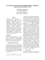
3.1 Overview
Our system can be divided into an offline and an online phase. In the offline
phase we create the data structures that allow for fast motion synthesis. In the
online phase these structures are queried and the resulting motion is rendered.
An overview is given in figure 3.1.
The offline phase (chapter 4) consists of the following steps:
1. We automatically segment a corpus of motion capture data into clips of

individual steps.
2. The clips are normalized by time warping, translating and rotating.
3. Automatic clean-up is applied to the clips.
4. We store these steps in a 3D parameter space S
low
using a Delaunay
Stride Space interpolation 15
3.1. OVERVIEW Sybren A. St¨uvel
OFFLINE PROCESS
ONLINE PROCESS
Motion capture lab
Input Animations
Conversion to alternative representation
Transformation to supporting frame
Normalization of durations
Query
Spanning neighbours
Blender
Interpolation
Foot fitting
Concatenation
Root fitting
Upper body filtering
Conversion to joint orientations
Produces
Database
User interface
Footstep planner
Individual steps
Walking animation

Final animation
Performs
Performs
Generator
Performs
Performs
Step Animations
Footstep detection
Figure 3.1: Global overview of the StrideSpace method.
16 Stride Space interpolation
Sybren A. St¨uvel CHAPTER 3. DESIGN AND IMPLEMENTATION
tetrahedralization. The steps in S
low
are represented in our alternative
body representation (chapter 6).
The parameter space S
low
is considered “low-dimensional” as it is an under-
parametrization of the footstep. It does not take orientation nor timing into
account. We use a higher dimensional distance function in section 5.1.
In the online phase (chapter 5) the user or footstep planner supplies a query
foot plan. Then, for each step in this query:
1. The query step is transformed to the lower-dimensional parameter repre-
sentation.
2. The system determines the blend candidates in S
low
. These are the ver-
tices of the tetrahedron containing the query step.
3. Based on these blend candidates, the system evaluates nearby blend can-
didates using a higher-dimensional distance function.

4. The final blend candidates are blended using both a rotational and posi-
tional interpolation scheme.
5. The generated step is aligned and fitted to the previous step.
3.2 Choice of parameter space
We discuss positions both in world coordinates and in a local coordinate system
called the supporting frame. The symbols used to denote the positions of the
feet are:
world local
Supporting foot W
sup
C
sup
Swing foot, initial position W
from
C
from
Swing foot, final position W
to
C
to
In order to add a footstep animation to the database, its parameters have to
be determined. These are determined based on the supporting foot W
sup
, the
initial position of the swing foot W
from
and the final position of the swing foot
W
to
. By assuming the step is performed on the ground plane, we can describe

the step by three parameters.
Stride Space interpolation 17
3.2. CHOICE OF PARAMETER SPACE Sybren A. St¨uvel
World coordinates Supporting frame coordinates
translate rotate
x
z
x
z
x
z
Figure 3.2: The transformation of a single step from world coordinates to sup-
porting frame coordinates
We can create a right-handed supporting foot coordinate frame, or supporting
frame for short, by applying a translation and a rotation to the animation
(figure 3.2). The transformation changes W
xxx
into C
xxx
. The origin of the
coordinate frame is placed at the supporting foot, C
from
lies on the (positive
or negative) x-axis and the y-axis is parallel to the ground plane orthogonal to
the x-axis, forming a right-handed coordinate system. C
from
is placed on the
positive x-axis when the right foot swings, and on the negative x-axis otherwise.
The parameter vector for the step is then given as:


P (W
sup
, W
from
, W
to
) =


C
from,x
C
to,x
C
to,z


18 Stride Space interpolation
Sybren A. St¨uvel CHAPTER 3. DESIGN AND IMPLEMENTATION
3.3 The Canonical Step
The Canonical Step is a single footstep animation in normalized form. Each
step starts and ends with a double stance, a posture in which both feet are
resting on the ground. There is always one supporting foot that remains on the
ground for the entire duration of the step; the other foot is called the swing foot.
Walking is generally distinguished from running in that there is always one foot
on the ground, and during a brief period between the swings both feet are.
The swing foot has two relevant positions, at the middle of each stance before
and after the swing, C
from
resp. C

to
. The supporting foot has only one position
C
sup
, as we assume it does not move during the step. It is determined at the
keyframe in the centre of the initial stance of the swing foot, i.e. at the same
moment in the animation C
from
is determined. The centre of the periods of
double support is used as we expect it to be the most representative of the start
and end location of the step. For deducing C
from
an earlier keyframe may be
influenced too much by the previous step in the original motion capture data,
and a later keyframe may already be part of the swing that was not recognised
as such by the footstep detector due to noise. A similar argument can be made
for C
to
.
The step’s local coordinate frame is positioned with the origin at the supporting
foot, the x-axis pointing at C
from
, the y-axis pointing upward through the foot,
and the z-axis orthogonal to both completing the right-handed frame. In other
words, the coordinate frame is chosen in the same way as the supporting frame
described in section 3.2. This means that C
sup
is always (0, 0, 0).
The canonical step also includes information about the durations of the swing
and the two periods of dual support. This information is used to determine

the speed of the blended step. The animation is timewarped in a piecewise
linear fashion to predefined durations and resampled before insertion into the
database. This ensures that all stored animations have the same duration and
the same number of frames, speeding up the blending process.
Stride Space interpolation 19
3.3. THE CANONICAL STEP Sybren A. St¨uvel
Step 2
Left foot
Right foot
Time
Swing
Stance
Swing
Stance
Stance
Step 1 Step 3
Swing
Figure 3.3: Schematic view of a walk. The yellow and blue areas represent those
moments in time where the left resp. right foot touches the ground. We blend
between steps in the periods of double support.
20 Stride Space interpolation
CHAPTER 4
Creating the Stride Space
In this chapter we elaborate on the offline construction of the parameter space.
This three-dimensional parameter space is called the Stride Space. We first look
at the way the input animations are segmented into separate steps in section 4.1.
Section 4.2 describes our three-dimensional database system. Section 4.3 tries
to answer questions like “how usable is my database for this technique?” and
“what steps are missing?”
4.1 Step segmentation

We extract individual steps from the motion capture data by determining the
moments at which the feet are planted. This in general is not trivial due to
noise and retargeting errors. The footstep detector needs to be precise in order
to get proper segmentation and eventually a decent parameterization. We use
a height- and velocity-based footstep detector[BE09].
The individual step animations are now converted to our alternative body re-
presentation. All operations are performed in this representation, until the
generated animation is handed over to the animation system.
Before determining the step’s parameters, every step is cleaned up. Foot skating
is removed by moving the root of every frame, such that the supporting foot is
placed at the origin. To be able to work with noisy motion capture data we also
adjust the feet to rest on the ground during the periods of support. Without
this step the feet could end up several centimeters above or below the ground
depending on the quality of the motion capture data and the parameters of
the footstep detector. The feet are moved only in the vertical axis, so these
Stride Space interpolation 21
4.2. THE DELAUNAY DATABASES Sybren A. St¨uvel
adjustments do not change the parameters of the step. The cleanup is done
automatically and does not require any manual action.
4.2 The Delaunay Databases
To perform location queries a Delaunay tetrahedralization is created from the
parameter points. Each parameter is a point in 3D space which makes the De-
launay tetrahedralization particularly useful. The Delaunay tetrahedralization
of the parameter points combined with references to the step animations and
metadata is called the Delaunay database. Performing a location query on the
database results in the tetrahedron spanned by four vertices. These vertices
are called the spanning neighbours and represent the parameters of the four
animations that will be blended into the final animation. The properties of the
Delaunay tetrahedralization ensure that those are four points that are relatively
similar to the query point.

The side of the swing foot determines the sign of the first parameter. Let
P
L
∈ R be the smallest real number such that first parameter C
from,x
of all
left steps are in the interval (−∞, p
L
]. Let P
R
∈ R be the largest real number
defined similarly for all right steps such that C
from,x
∈ [p
R
, ∞). When all blend
candidates are inserted into the same database, querying in the interval [p
L
, p
R
]
may result in a mixture of left and right steps being blended. To prevent this,
we separate the database in two parts, one for each side of the swing foot. As a
result of this separation, extrapolation is necessary to process a query for a left
step in the interval (p
L
, ∞) or a right step in (−∞, P
R
).
There are many ways in which walking animations can be classified, such as

walking forward, turning, side-stepping and walking backwards. However, these
classifications are not distinct; walking forward and decreasing the length of
the swing results in slowing down and gradually results in walking backward.
The same holds for the possibly gradual changes between walking straight and
turning sharply. This means that it is impractical to separate the database even
further based on these classifications. To decrease the likeliness that steps of dif-
ferent classifications are blended we use a higher-dimensional distance function
– see section 5.1.
22 Stride Space interpolation
Sybren A. St¨uvel CHAPTER 4. CREATING THE STRIDE SPACE
Figure 4.1: Visualization of the left-step and right-step Delaunay databases with
a query point.
Stride Space interpolation 23
4.3. DATABASE ANALYSIS Sybren A. St¨uvel
4.3 Database analysis
As our technique interpolates between steps, the largest steps in the database
have to be larger than any of the query steps, and similar for small steps. We
have provided an analysis algorithm that detects such potential problems. Previ-
ous studies [Hof65][EB79] have shown a relation between stride length (SL) and
the trochanterion height (TH). When sprinting at 2.5 m/s the average SL:TH
ratio was shown to be 1.10 for males and 1.11 for females. Tripathy [Tri04] mea-
sured an average ratio of 0.65 when walking. In our analysis of the database we
use a SL:TH ratio of 1.0 to determine the maximum stride length.
We do not only look at the step length, but also regard the width of the stances,
i.e. the distance between the feet. It is possible for a step to end smaller or
larger than any step starts. This means that it is impossible to continue walking
from such a step without resorting to extrapolation. The manually constructed
foot plans have been constructed to avoid this situation.
Even though our database did not have a wide enough gamut to allow for a full
spectrum of steps, it was nevertheless usable for the examples we have shown.

Figure 4.3 shows the projection of the left-side database in the p
2
/p
3
plane. The
white disc in the centre represents the supporting right foot. The centres of the
yellow discs represent the coordinates in the supporting frame of the final double
stance, i.e. C
to
. The radius of the yellow discs reflects the area in which this
step is considered to be similar to other steps, which we have taken to be 15cm
based on the size of a human foot. The blue circle represents the maximum
step size as described above. Of course the parameters for the analysis can be
adjusted for individual needs.
This is the output of the analysis software. A sidestep is defined as a step where
the sideways movement of the swing foot is more than three times the forward
movement. There is a chance of a sidestep being blended with a 180
o
turn,
which is why it is important to have sidesteps that end small in the database.
24 Stride Space interpolation
Sybren A. St¨uvel CHAPTER 4. CREATING THE STRIDE SPACE
Importing /final-bvh/L-test.cgal
Loading 94 vertices
Loaded left-step database, inverting XY-parameters.
You have a high enough density of steps that start small.
You have a high enough density of steps that start wide.
You should have steps that start smaller.
The smallest width in DB is 18.0 cm but should be at most 15.0 cm
You should have steps that start wider.

The widest width in DB is 77.2 cm but should be at least 95.0 cm
You have a high enough density of steps that end small.
You have a high enough density of steps that end wide.
You should have steps that end smaller.
The smallest width in DB is 18.4 cm but should be at most 15.0 cm
You should have steps that end wider.
The widest width in DB is 90.2 cm but should be at least 95.0 cm
Found 36 sidesteps.
You have no sidesteps that start small enough.
Minimal width in DB is 18.7 cm, should be at most 15.0 cm
You have no sidesteps that end small enough.
Minimal width in DB is 21.3 cm, should be at most 15.0 cm
You have a step that ends with the feet 90.2 cm apart, and 0 steps
that start with that width or wider. You need at least 3 steps
that are wider. The widest so far is 77.2 cm wide.
Figure 4.2: Output of the database analysis algorithm.
Figure 4.3: Projection of the p
2
/p
3
plane of the left-side Delaunay database.
Stride Space interpolation 25