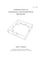
Introduction to lagrangian and hamiltonian mechanics BRIZARD, a j

July 14, 2004
INTRODUCTION TO
LAGRANGIAN AND HAMILTONIAN
MECHANICS
Alain J. Brizard
Department of Chemistry and Physics
Saint Michael’s College, Colchester, VT 05439
Contents
1 Introduction to the Calculus of Variations 1
1.1 Fermat’s Principle of Least Time . . . . . . . . . . . . . . . . . . . . . . . 1
1.1.1 Euler’s First Equation . . . . . . . . . . . . . . . . . . . . . . . . . 3
1.1.2 Euler’s Second Equation . . . . . . . . . . . . . . . . . . . . . . . . 5
1.1.3 Snell’sLaw 6
1.1.4 Application of Fermat’s Principle . . . . . . . . . . . . . . . . . . . 7
1.2 Geometric Formulation of Ray Optics . . . . . . . . . . . . . . . . . . . . . 9
1.2.1 Frenet-Serret Curvature of Light Path . . . . . . . . . . . . . . . . 9
1.2.2 Light Propagation in Spherical Geometry . . . . . . . . . . . . . . . 11
1.2.3 Geodesic Representation of Light Propagation . . . . . . . . . . . . 13
1.2.4 Eikonal Representation . . . . . . . . . . . . . . . . . . . . . . . . . 15
1.3 Brachistochrone Problem . . . . . . . . . . . . . . . . . . . . . . . . . . . . 15
1.4 Problems 18
2 Lagrangian Mechanics 21
2.1 Maup ertuis-Jacobi Principle of Least Action . . . . . . . . . . . . . . . . . 21
2.2 Principle of Least Action of Euler and Lagrange . . . . . . . . . . . . . . . 23
2.2.1 Generalized Coordinates in Configuration Space . . . . . . . . . . . 23
2.2.2 Constrained Motion on a Surface . . . . . . . . . . . . . . . . . . . 24
2.2.3 Euler-Lagrange Equations . . . . . . . . . . . . . . . . . . . . . . . 25
2.3 Lagrangian Mechanics in Configuration Space . . . . . . . . . . . . . . . . 27
2.3.1 Example I: Pendulum . . . . . . . . . . . . . . . . . . . . . . . . . . 27
i
ii CONTENTS

2.3.2 Example II: Bead on a Rotating Hoop . . . . . . . . . . . . . . . . 28
2.3.3 Example III: Rotating Pendulum . . . . . . . . . . . . . . . . . . . 30
2.3.4 Example IV: Compound Atwood Machine . . . . . . . . . . . . . . 31
2.3.5 Example V: Pendulum with Oscillating Fulcrum . . . . . . . . . . . 33
2.4 Symmetries and Conservation Laws . . . . . . . . . . . . . . . . . . . . . . 35
2.4.1 Energy Conservation Law . . . . . . . . . . . . . . . . . . . . . . . 36
2.4.2 Momentum Conservation Law . . . . . . . . . . . . . . . . . . . . . 36
2.4.3 Invariance Prop erties . . . . . . . . . . . . . . . . . . . . . . . . . . 36
2.4.4 Lagrangian Mechanics with Symmetries . . . . . . . . . . . . . . . 38
2.4.5 Routh’s Procedure for Eliminating Ignorable Coordinates . . . . . . 39
2.5 Lagrangian Mechanics in the Center-of-Mass Frame . . . . . . . . . . . . . 40
2.6 Problems 43
3 Hamiltonian Mechanics 45
3.1 Canonical Hamilton’s Equations . . . . . . . . . . . . . . . . . . . . . . . . 45
3.2 Legendre Transformation . . . . . . . . . . . . . . . . . . . . . . . . . . . . 46
3.3 Hamiltonian Optics and Wave-Particle Duality* . . . . . . . . . . . . . . . 48
3.4 Particle Motion in an Electromagnetic Field* . . . . . . . . . . . . . . . . . 49
3.4.1 Euler-Lagrange Equations . . . . . . . . . . . . . . . . . . . . . . . 49
3.4.2 Energy Conservation Law . . . . . . . . . . . . . . . . . . . . . . . 50
3.4.3 Gauge Invariance . . . . . . . . . . . . . . . . . . . . . . . . . . . . 51
3.4.4 Canonical Hamilton’s Equationss . . . . . . . . . . . . . . . . . . . 51
3.5 One-degree-of-freedom Hamiltonian Dynamics . . . . . . . . . . . . . . . . 52
3.5.1 Simple Harmonic Oscillator . . . . . . . . . . . . . . . . . . . . . . 53
3.5.2 Pendulum 54
3.5.3 Constrained Motion on the Surface of a Cone . . . . . . . . . . . . 56
3.6 Charged Spherical Pendulum in a Magnetic Field* . . . . . . . . . . . . . . 57
3.6.1 Lagrangian . . . . . . . . . . . . . . . . . . . . . . . . . . . . . . . 57
3.6.2 Euler-Lagrange equations . . . . . . . . . . . . . . . . . . . . . . . 59
CONTENTS iii
3.6.3 Hamiltonian . . . . . . . . . . . . . . . . . . . . . . . . . . . . . . . 60

3.7 Problems 65
4 Motion in a Central-Force Field 67
4.1 Motion in a Central-Force Field . . . . . . . . . . . . . . . . . . . . . . . . 67
4.1.1 Lagrangian Formalism . . . . . . . . . . . . . . . . . . . . . . . . . 67
4.1.2 Hamiltonian Formalism . . . . . . . . . . . . . . . . . . . . . . . . . 69
4.1.3 Turning Points . . . . . . . . . . . . . . . . . . . . . . . . . . . . . 70
4.2 Homogeneous Central Potentials* . . . . . . . . . . . . . . . . . . . . . . . 70
4.2.1 The Virial Theorem . . . . . . . . . . . . . . . . . . . . . . . . . . . 71
4.2.2 General Properties of Homogeneous Potentials . . . . . . . . . . . . 72
4.3 KeplerProblem 72
4.3.1 Bounded Keplerian Orbits . . . . . . . . . . . . . . . . . . . . . . . 73
4.3.2 Unbounded Keplerian Orbits . . . . . . . . . . . . . . . . . . . . . . 76
4.3.3 Laplace-Runge-Lenz Vector* . . . . . . . . . . . . . . . . . . . . . . 77
4.4 Isotropic Simple Harmonic Oscillator . . . . . . . . . . . . . . . . . . . . . 78
4.5 Internal Reflection inside a Well . . . . . . . . . . . . . . . . . . . . . . . . 80
4.6 Problems 83
5 Collisions and Scattering Theory 85
5.1 Two-Particle Collisions in the LAB Frame . . . . . . . . . . . . . . . . . . 85
5.2 Two-Particle Collisions in the CM Frame . . . . . . . . . . . . . . . . . . . 87
5.3 Connection between the CM and LAB Frames . . . . . . . . . . . . . . . . 88
5.4 Scattering Cross Sections . . . . . . . . . . . . . . . . . . . . . . . . . . . . 90
5.4.1 Definitions . . . . . . . . . . . . . . . . . . . . . . . . . . . . . . . . 90
5.4.2 Scattering Cross Sections in CM and LAB Frames . . . . . . . . . . 91
5.5 Rutherford Scattering . . . . . . . . . . . . . . . . . . . . . . . . . . . . . . 93
5.6 Hard-Sphere and Soft-Sphere Scattering . . . . . . . . . . . . . . . . . . . 94
5.6.1 Hard-Sphere Scattering . . . . . . . . . . . . . . . . . . . . . . . . . 95
iv CONTENTS
5.6.2 Soft-Sphere Scattering . . . . . . . . . . . . . . . . . . . . . . . . . 96
5.7 Problems 99
6 Motion in a Non-Inertial Frame 103

6.1 Time Derivatives in Fixed and Rotating Frames . . . . . . . . . . . . . . . 103
6.2 Accelerations in Rotating Frames . . . . . . . . . . . . . . . . . . . . . . . 105
6.3 Lagrangian Formulation of Non-Inertial Motion . . . . . . . . . . . . . . . 106
6.4 Motion Relative to Earth . . . . . . . . . . . . . . . . . . . . . . . . . . . . 108
6.4.1 Free-Fall Problem Revisited . . . . . . . . . . . . . . . . . . . . . . 111
6.4.2 Foucault Pendulum . . . . . . . . . . . . . . . . . . . . . . . . . . . 112
6.5 Problems 116
7 Rigid Body Motion 117
7.1 InertiaTensor 117
7.1.1 Discrete Particle Distribution . . . . . . . . . . . . . . . . . . . . . 117
7.1.2 Parallel-Axes Theorem . . . . . . . . . . . . . . . . . . . . . . . . . 119
7.1.3 Continuous Particle Distribution . . . . . . . . . . . . . . . . . . . 120
7.1.4 Principal Axes of Inertia . . . . . . . . . . . . . . . . . . . . . . . . 122
7.2 Angular Momentum . . . . . . . . . . . . . . . . . . . . . . . . . . . . . . 124
7.2.1 Euler Equations . . . . . . . . . . . . . . . . . . . . . . . . . . . . . 124
7.2.2 Euler Equations for a Force-Free Symmetric Top . . . . . . . . . . . 125
7.2.3 Euler Equations for a Force-Free Asymmetric Top . . . . . . . . . . 127
7.3 Symmetric Top with One Fixed Point . . . . . . . . . . . . . . . . . . . . . 130
7.3.1 Eulerian Angles as generalized Lagrangian Co ordinates . . . . . . . 130
7.3.2 Angular Velocity in terms of Eulerian Angles . . . . . . . . . . . . . 131
7.3.3 Rotational Kinetic Energy of a Symmetric Top . . . . . . . . . . . . 132
7.3.4 Lagrangian Dynamics of a Symmetric Top with One Fixed Point . . 133
7.3.5 Stability of the Sleeping Top . . . . . . . . . . . . . . . . . . . . . . 139
7.4 Problems 140
CONTENTS v
8 Normal-Mode Analysis 143
8.1 Stability of Equilibrium Points . . . . . . . . . . . . . . . . . . . . . . . . . 143
8.1.1 Bead on a Rotating Hoop . . . . . . . . . . . . . . . . . . . . . . . 143
8.1.2 Circular Orbits in Central-Force Fields . . . . . . . . . . . . . . . . 144
8.2 Small Oscillations about Stable Equilibria . . . . . . . . . . . . . . . . . . 145

8.3 Coupled Oscillations and Normal-Mo de Analysis . . . . . . . . . . . . . . . 146
8.3.1 Coupled Simple Harmonic Oscillators . . . . . . . . . . . . . . . . . 146
8.3.2 Nonlinear Coupled Oscillators . . . . . . . . . . . . . . . . . . . . . 147
8.4 Problems 150
9 Continuous Lagrangian Systems 155
9.1 Waves on a Stretched String . . . . . . . . . . . . . . . . . . . . . . . . . . 155
9.1.1 Wave Equation . . . . . . . . . . . . . . . . . . . . . . . . . . . . . 155
9.1.2 Lagrangian Formalism . . . . . . . . . . . . . . . . . . . . . . . . . 155
9.1.3 Lagrangian Description for Waves on a Stretched String . . . . . . 156
9.2 General Variational Principle for Field Theory . . . . . . . . . . . . . . . . 157
9.2.1 Action Functional . . . . . . . . . . . . . . . . . . . . . . . . . . . . 157
9.2.2 Noether Method and Conservation Laws . . . . . . . . . . . . . . . 158
9.3 Variational Principle for Schroedinger Equation . . . . . . . . . . . . . . . 159
9.4 Variational Principle for Maxwell’s Equations* . . . . . . . . . . . . . . . . 161
9.4.1 Maxwell’s Equations as Euler-Lagrange Equations . . . . . . . . . . 161
9.4.2 Energy Conservation Law for Electromagnetic Fields . . . . . . . . 163
A Notes on Feynman’s Quantum Mechanics 165
A.1 Feynman postulates and quantum wave function . . . . . . . . . . . . . . . 165
A.2 Derivation of the Schroedinger equation . . . . . . . . . . . . . . . . . . . . 166
Chapter 1
Introduction to the Calculus of
Variations
Minimum principles have been invoked throughout the history of Physics to explain the
behavior of light and particles. In one of its earliest form, Heron of Alexandria (ca. 75
AD) stated that light travels in a straight line and that light follows a path of shortest
distance when it is reflected by a mirror. In 1657, Pierre de Fermat (1601-1665) stated
the Principle of Least Time, whereby light travels between two points along a path that
minimizes the travel time, to explain Snell’s Law (Willebrord Snell, 1591-1626) associated
with light refraction in a stratified medium.
The mathematical foundation of the Principle of Least Time was later developed by

Joseph-Louis Lagrange (1736-1813) and Leonhard Euler (1707-1783), who developed the
mathematical method known as the Calculus of Variations for finding curves that minimize
(or maximize) certain integrals. For example, the curve that maximizes the area enclosed
by a contour of fixed length is the circle (e.g., a circle encloses an area 4/π times larger
than the area enclosed by a square of equal perimeter length). The purpose of the present
Chapter is to introduce the Calculus of Variations by means of applications of Fermat’s
Principle of Least Time.
1.1 Fermat’s Principle of Least Time
According to Heron of Alexandria, light travels in a straight line when it propagates in a
uniform medium. Using the index of refraction n
0
≥ 1 of the uniform medium, the speed of
light in the medium is expressed as v
0
= c/n
0
≤ c, where c is the speed of light in vacuum.
This straight path is not only a path of shortest distance but also a path of least time.
According to Fermat’s Principle (Pierre de Fermat, 1601-1665), light propagates in a
nonuniform medium by travelling along a path that minimizes the travel time between an
1
2 CHAPTER 1. INTRODUCTION TO THE CALCULUS OF VARIATIONS
Figure 1.1: Light path in a nonuniform medium
initial p oint A (where a light ray is launched) and a final point B (where the light ray is
received). Hence, the time taken by a light ray following a path γ from point A to point
B (parametrized by σ)is
T
γ
=


γ
c
−1
n(x)





dx
dσ





dσ = c
−1
L
γ
, (1.1)
where L
γ
represents the length of the optical path taken by light. In Sections 1 and 2 of
the present Chapter, we consider ray propagation in two dimensions and return to general
properties of ray propagation in Section 3.
For ray propagation in two dimensions (labeled x and y) in a medium with nonuniform
refractive index n(y), an arbitrary point (x, y = y(x)) along the light path γ is parametrized
by the x-coordinate [i.e., σ = x in Eq. (1.1)], which starts at point A =(a, y
a

) and ends at
point B =(b,y
b
) (see Figure 1.1). Note that the path γ is now represented by the mapping
y : x → y(x). Along the path γ, the infinitesimal length element is ds =

1+(y

)
2
dx
along the path y(x) and the optical length
L[y]=

b
a
n(y)

1+(y

)
2
dx (1.2)
is now a functional of y (i.e., changing y changes the value of the integral L[y]).
For the sake of convenience, we introduce the function
F (y,y

; x)=n(y)

1+(y


)
2
(1.3)
to denote the integrand of Eq. (1.2); here, we indicate an explicit dependence on x of
F (y,y

; x) for generality.
1.1. FERMAT’S PRINCIPLE OF LEAST TIME 3
Figure 1.2: Virtual displacement
1.1.1 Euler’s First Equation
We are interested in finding the curve y(x) that minimizes the optical-path integral (1.2).
The method of Calculus of Variations will transform the problem of minimizing an integral
of the form

b
a
F (y,y

; x) dx into the solution of a differential equation expressed in terms
of derivatives of the integrand F (y,y

; x).
To determine the path of least time, we introduce the functional derivative δL[y] defined
as
δL[y]=

d
d
L[y + δy]


=0
,
where δy(x) is an arbitrary smooth variation of the path y(x) subject to the boundary
conditions δy(a)=0=δy(b). Hence, the end points of the path are not affected by the
variation (see Figure 1.2). Using the expression for L[y] in terms of the function F (y, y

; x),
we find
δL[y]=

b
a

δy(x)
∂F
∂y(x)
+ δy

(x)
∂F
∂y

(x)

dx,
where δy

=(δy)


, which when integrated by parts becomes
δL[y]=

b
a
δy

∂F
∂y
−
d
dx

∂F
∂y


dx +
1
c

δy
b

∂F
∂y


b
− δy

a

∂F
∂y


a

.
Here, since the variation δy(x) vanishes at the integration boundaries (δy
b
=0=δy
a
),
we obtain
δL[y]=

b
a
δy

∂F
∂y
−
d
dx

∂F
∂y



dx. (1.4)
4 CHAPTER 1. INTRODUCTION TO THE CALCULUS OF VARIATIONS
The condition that the path γ takes the least time, corresponding to the variational principle
δL[y] = 0, yields Euler’s First equation
d
dx

∂F
∂y


=
∂F
∂y
. (1.5)
This ordinary differential equation for y(x) yields a solution that gives the desired path of
least time.
We now apply the variational principle δL[y] = 0 for the case where F is given by
Eq. (1.3), for which we find
∂F
∂y

=
n(y) y


1+(y

)

2
and
∂F
∂y
= n

(y)

1+(y

)
2
,
so that Euler’s First Equation (1.5) becomes
n(y) y

= n

(y)

1+(y

)
2

. (1.6)
Although the solution of this (nonlinear) second-order ordinary differential equation is
difficult to obtain for general functions n(y), we can nonetheless obtain a qualitative picture
of its solution by noting that y


has the same sign as n

(y). Hence, when n

(y) = 0 (i.e., the
medium is spatially uniform), the solution y

= 0 yields the straight line y(x; φ
0
)=tanφ
0
x,
where φ
0
denotes the initial launch angle (as measured from the horizontal axis). The case
where n

(y) > 0 (or n

(y) < 0), on the other hand, yields a light path which is concave
upwards (or downwards) as will be shown below.
We should point out that Euler’s First Equation (1.5) results from the extremum condi-
tion δL[y] = 0, which does not necessarily imply that the Euler path y(x) actually minimizes
the optical length L[y]. To show that the path y(x) minimizes the optical length L[y], we
must evaluate the second functional derivative
δ
2
L[y]=

d

2
d
2
L[y + δy]

=0
.
By following steps similar to the derivation of Eq. (1.4), we find
δ
2
L[y]=

b
a

δy
2

∂
2
F
∂y
2
−
d
dx

∂
2
F

∂y∂y


+(δy

)
2
∂
2
F
∂(y

)
2

.
The necessary and sufficient condition for a minimum is δ
2
L>0 and, thus, the sufficient
conditions for a minimal optical length are
∂
2
F
∂y
2
−
d
dx

∂

2
F
∂y∂y


> 0 and
∂
2
F
∂(y

)
2
> 0,
1.1. FERMAT’S PRINCIPLE OF LEAST TIME 5
for all smo oth variations δy(x). Using Eqs. (1.3) and (1.6), we find
∂
2
F
(∂y

)
2
=
n
[1 + (y

)
2
]

3/2
> 0
and
∂
2
F
∂y
2
= n


1+(y

)
2
and
∂
2
F
∂y ∂y

=
n

y


1+(y

)

2
so that
∂
2
F
∂y
2
−
d
dx

∂
2
F
∂y∂y


=
n
2
F
d
2
ln n
dy
2
.
Hence, the sufficient condition for a minimal optical length for light traveling in a nonuni-
form refractive medium is d
2

ln n/dy
2
> 0.
1.1.2 Euler’s Second Equation
Under certain conditions, we may obtain a partial solution to Euler’s First Equation (1.6)
for a light path y(x) in a nonuniform medium. This partial solution is provided by Euler’s
Second equation, which is derived as follows.
First, we write the exact derivative dF/dx for F (y,y

; x)as
dF
dx
=
∂F
∂x
+ y

∂F
∂y
+ y

∂F
∂y

,
and substitute Eq. (1.5) to combine the last two terms so that we obtain Euler’s Second
equation
d
dx


F − y

∂F
∂y


=
∂F
∂x
. (1.7)
In the present case, the function F (y,y

; x), given by Eq. (1.3), is explicitly independent of
x (i.e., ∂F/∂x = 0), and we find
F − y

∂F
∂y

=
n(y)

1+(y

)
2
= constant,
and thus the partial solution of Eq. (1.6) is
n(y)=α


1+(y

)
2
, (1.8)
where α is a constant determined from the initial conditions of the light ray; note that,
since the right side of Eq. (1.8) is always greater than α, we find that n( y) >α. This is
indeed a partial solution (in some sense), since we have reduced the derivative order from
6 CHAPTER 1. INTRODUCTION TO THE CALCULUS OF VARIATIONS
second-order derivative in Eq. (1.6) to first-order derivative in Eq. (1.8): y

(x) → y

(x)on
the solution y(x).
Euler’s Second Equation has, thus, produced an equation of the form G(y,y

; x)=0,
which can normally be integrated by quadrature. Here, Eq. (1.8) can be integrated by
quadrature to give the integral solution
x(y)=

y
0
αdη

[n(η)]
2
− α
2

, (1.9)
subject to the condition x(y = 0) = 0. From the explicit dependence of the index of
refraction n(y), one may be able to perform the integration in Eq. (1.9) to obtain x(y) and,
thus, obtain an explicit solution y(x) by inverting x(y).
For example, let us consider the path associated with the index of refraction n(y)=H/y,
where the height H is a constant and 0 <y<Hα
−1
to ensure that, according to Eq. (1.8),
n(y) >α. The integral (1.9) can then be easily integrated to yield
x(y)=

y
0
αηdη

H
2
− (αη)
2
= Hα
−1


1 −

1 −

αy
H


2


.
Hence, the light path simply forms a semi-circle of radius R = α
−1
H centered at (x, y)=
(R, 0):
(R −x)
2
+ y
2
= R
2
→ y(x)=

x (2R −x).
The light path is indeed concave downward since n

(y) < 0.
Returning to Eq. (1.8), we note that it states that as a light ray enters a region of
increased (decreased) refractive index, the slope of its path also increases (decreases). In
particular, by substituting Eq. (1.6) into Eq. (1.8), we find
α
2
y

=
1
2

dn
2
(y)
dy
,
and, hence, the path of a light ray is concave upward (downward) where n

(y) is positive
(negative), as previously discussed.
1.1.3 Snell’s Law
Let us now consider a light ray travelling in two dimensions from (x, y)=(0, 0) at an angle
φ
0
(measured from the x-axis) so that y

(0) = tan φ
0
is the slop e at x = 0, assuming that
y(0) = 0. The constant α is then simply determined from initial conditions as
α = n
0
cos φ
0
,
1.1. FERMAT’S PRINCIPLE OF LEAST TIME 7
where n
0
= n(0) is the refractive index at y(0) = 0. Next, let y

(x) = tan φ(x) be the slop e

of the light ray at (x, y(x)), then

1+(y

)
2
= sec φ and Eq. (1.8) becomes n(y) cos φ =
n
0
cos φ
0
, which, when we substitute the complementary angle θ = π/2 − φ, finally yields
the standard form of Snell’s Law:
n[y(x)] sin θ(x)=n
0
sin θ
0
, (1.10)
properly generalized to include a light path in a nonuniform refractive medium. Note that
Snell’s Law does not tell us anything about the actual light path y(x); this solution must
come from solving Eq. (1.9).
1.1.4 Application of Fermat’s Principle
As an application of the Principle of Least Time, we consider the propagation of a light
ray in a medium with refractive index n(y)=n
0
(1 − βy) exhibiting a constant gradient
n

(y)=−n
0

β.
Once again with α = n
0
cos φ
0
and y

(0) = tan φ
0
, Eq. (1.8) becomes
1 − βy = cos φ
0

1+(y

)
2
.
By separating dy and dx we obtain
dx =
cos φ
0
dy

(1 −βy)
2
− cos
2
φ
0

. (1.11)
We now use the trigonometric substitution
1 −βy= cos φ
0
sec θ, (1.12)
with θ = φ
0
at y = 0, to find
dy = −
cos φ
0
β
sec θ tan θdθ
and

(1 −βy)
2
− cos
2
φ
0
= cos φ
0
tan θ,
so that Eq. (1.11) becomes
dx = −
cos φ
0
β
sec θdθ. (1.13)

The solution to this equation, with x = 0 when θ = φ
0
,is
x = −
cos φ
0
β
ln

sec θ + tan θ
sec φ
0
+ tan φ
0

. (1.14)
8 CHAPTER 1. INTRODUCTION TO THE CALCULUS OF VARIATIONS
If we can now solve for sec θ as a function of x from Eq. (1.14), we can substitute this
solution into Eq. (1.12) to obtain an expression for the light path y(x). For this purpose,
we define
ψ =
βx
cos φ
0
− ln(sec φ
0
+ tan φ
0
),
so that Eq. (1.14) becomes

sec θ +
√
sec
2
θ − 1=e
− ψ
,
which can be solved for sec θ as
sec θ = cosh ψ = cosh

βx
cos φ
0
− ln(sec φ
0
+ tan φ
0
)

.
Substituting this equation into Eq. (1.12), we find the light path
y(x; β)=
1
β
−
cos φ
0
β
cosh


βx
cos φ
0
− ln(sec φ
0
+ tan φ
0
)

. (1.15)
Note that, using the identities
cosh [ln(sec φ
0
+ tan φ
0
)] = sec φ
0
sinh [ln(sec φ
0
+ tan φ
0
)] = tan φ
0





, (1.16)
we can check that, in the uniform case (β = 0), we recover the expected result

lim
β→0
y(x; β) = (tan φ
0
) x.
Next, we observe that y(x; β) exhibits a single maximum located at x = x(β). Solving
for x(β) from y

(x; β) = 0, we obtain
tanh

β x
cos φ
0

= sin φ
0
,
or
x(β)=
cos φ
0
β
ln(sec φ
0
+ tan φ
0
), (1.17)
and hence
y(x; β)=

1
β
−
cos φ
0
β
cosh

β
cos φ
0
(x −x)

,
and
y(β)=y(x; β)=(1− cos φ
0
)/β. Figure 1.3 shows a graph of the normalized solution
y(x; β)/y(β) as a function of the normalized coordinate x/x(β) for φ
0
=
π
3
.
1.2. GEOMETRIC FORMULATION OF RAY OPTICS 9
Figure 1.3: Light-path solution for a linear nonuniform medium
1.2 Geometric Formulation of Ray Optics
1.2.1 Frenet-Serret Curvature of Light Path
We now return to the general formulation for light-ray propagation based on the time
integral (1.1), where the integrand is

F

x,
dx
dσ

= n(x)





dx
dσ





,
where light rays are now allowed to travel in three-dimensional space and the index of
refraction n(x) is a general function of position. Euler’s First equation in this case is
d
dσ

∂F
∂(dx/dσ)

=
∂F

∂x
, (1.18)
where
∂F
∂(dx/dσ)
=
n
λ
dx
dσ
and
∂F
∂x
= λ ∇n,
with
λ =





dx
dσ





=






dx
dσ

2
+

dy
dσ

2
+

dz
dσ

2
.
Euler’s First Equation (1.18), therefore, becomes
d
dσ

n
λ
dx
dσ


= λ ∇n. (1.19)
10 CHAPTER 1. INTRODUCTION TO THE CALCULUS OF VARIATIONS
Euler’s Second Equation, on the other hand, states that
F −
dx
dσ
·
∂F
∂(dx/dσ)
=0
is a constant of motion.
By choosing the ray parametrization dσ = ds (so that λ = 1), we find that the ray
velocity dx/ds =

k is a unit vector which defines the direction of the wave vector k. With
this parametrization, Euler’s equation (1.19) is now replaced with
d
ds

n
dx
ds

= ∇n →
d
2
x
ds
2
=

dx
ds
×

∇ln n ×
dx
ds

. (1.20)
Eq. (1.20) shows that the Frenet-Serret curvature of the light path is |∇ln n ×

k | (and its
radius of curvature is |∇ln n ×

k |
−1
) while the path has zero torsion since it is planar.
Eq. (1.20) can also be written in geometric form by introducing the metric relation
ds
2
= g
ij
dx
i
dx
j
, where g
ij
= e
i

· e
j
denotes the metric tensor defined in terms of the
contravariant-basis vectors (e
1
, e
2
, e
3
), so that
dx
ds
=
dx
i
ds
e
i
.
Using the definition for the Christoffel symb ol
Γ

jk
=
1
2
g
i

∂g

ij
∂x
k
+
∂g
ik
∂x
j
−
∂g
jk
∂x
i

,
where g
ij
denotes a component of the inverse metric (i.e., g
ij
g
jk
= δ
i
k
), we find the relations
de
j
ds
=Γ
i

jk
dx
k
ds
e
i
,
and
d
2
x
ds
2
=
d
2
x
i
ds
2
e
i
+
dx
i
ds
de
i
ds
=


d
2
x
i
ds
2
+Γ
i
jk
dx
j
ds
dx
k
ds

e
i
.
By combining these relations, Eq. (1.20) becomes
d
2
x
i
ds
2
+Γ
i
jk

dx
j
ds
dx
k
ds
=

g
ij
−
dx
i
ds
dx
j
ds

∂ ln n
∂x
j
, (1.21)
Looking at Figure 1.4, we see that the light ray bends towards regions of higher index
of refraction. Note that, if we introduce the unit vector

n = ∇n/(|∇n|) pointing in the
direction of increasing index of refraction, we find the equation
d
ds



n × n
dx
ds

=
d
ds


n × n

k

=
d

n
ds
× n

k,
1.2. GEOMETRIC FORMULATION OF RAY OPTICS 11
Figure 1.4: Light curvature
where we have used Eq. (1.20) to obtain

n ×
d
ds


n
dx
ds

=

n × ∇n =0.
Hence, if the direction

n is constant along the path of a light ray (i.e., d

n/ds = 0), then the
quantity

n × n

k is a constant. In addition, when a light ray progagates in two dimensions,
this conservation law implies that the quantity |

n × n

k| = n sin θ is also a constant, which
is none other than Snell’s Law (1.10).
1.2.2 Light Propagation in Spherical Geometry
By using the general ray-orbit equation (1.20), we can also show that for a spherically-
symmetric nonuniform medium with index of refraction n(r), the light-ray orbit r(s) sat-
isfies the conservation law
d
ds


r × n(r)
dr
ds

=0. (1.22)
Here, we use the fact that the ray-orbit path is planar and, thus, we write
r ×
dr
ds
= r sin φ

z, (1.23)
where φ denotes the angle between the position vector r and the tangent vector dr/ds (see
Figure 1.5). The conservation law (1.22) for ray orbits in a spherically-symmetric medium
12 CHAPTER 1. INTRODUCTION TO THE CALCULUS OF VARIATIONS
Figure 1.5: Light path in a nonuniform medium with spherical symmetry
can, therefore, be expressed as
n(r) r sin φ(r)=Na,
where N and a are constants (determined from initial conditions); note that the condition
n(r) r>Namust be satisfied.
An explicit expression for the ray orbit r( θ) is obtained as follows. First, since dr/ds is
a unit vector, we find
dr
ds
=
dθ
ds

r


θ +
dr
dθ

r

=
r

θ +(dr/dθ)

r

r
2
+(dr/dθ)
2
,
so that
dθ
ds
=
1

r
2
+(dr/dθ)
2
and Eq. (1.23) yields
r ×

dr
ds
= r sin φ

z = r
2
dθ
ds

z → sinφ =
r

r
2
+(dr/dθ)
2
=
Na
nr
.
Next, integration by quadrature yields
dr
dθ
=
r
Na

n(r)
2
r

2
− N
2
a
2
→ θ(r)=Na

r
r
0
dρ
ρ

n
2
(ρ) ρ
2
−N
2
a
2
,
1.2. GEOMETRIC FORMULATION OF RAY OPTICS 13
where θ(r
0
) = 0. Lastly, a change of integration variable η = Na/ρ yields
θ(r)=

Na/r
0

Na/r
dη

n
2
(η) −η
2
, (1.24)
where
n(η) ≡ n(Na/η).
Consider, for example, the spherically-symmetric refractive index
n(r)=n
0

2 −
r
2
R
2
→ n
2
(η)=n
2
0

2 −
N
2

2

η
2

,
where n
0
= n(R) denotes the refractive index at r = R and  = a/R is a dimensionless
parameter. Hence, Eq. (1.24) becomes
θ(r)=

Na/r
0
Na/r
ηdη

2n
2
0
η
2
− n
2
0
N
2

2
− η
4
=

1
2

(Na/r
0
)
2
(Na/r)
2
dσ

n
4
0
e
2
− (σ −n
2
0
)
2
,
where e =

1 −N
2

2
/n
2

0
(assuming that n
0
>N). Using the trigonometric substitution
σ = n
2
0
(1 + e cos χ), we find
θ(r)=
1
2
χ(r) → r
2
(θ)=
r
2
0
(1 + e)
1+e cos 2θ
,
which represents an ellipse of major radius and minor radius
r
1
= R (1 + e)
1/2
and r
0
= R (1 −e)
1/2
resp ectively. The angle φ(θ) defined from the conservation law (1.22) is now expressed as

sin φ(θ)=
1+e cos 2θ
√
1+e
2
+2e cos 2θ
,
so that φ =
π
2
at θ =0and
π
2
, as expected for an ellipse.
1.2.3 Geodesic Representation of Light Propagation
We now investigate the geodesic properties of light propagation in a nonuniform refractive
medium. For this purpose, let us consider a path AB in space from point A to point B
parametrized by the continuous parameter σ, i.e., x(σ) such that x(A)=x
A
and x(B)=
x
B
. The time taken by light in propagating from A to B is
T
AB
=

B
A
dt

dσ
dσ =

B
A
n
c

g
ij
dx
i
dσ
dx
j
dσ

1/2
dσ, (1.25)
14 CHAPTER 1. INTRODUCTION TO THE CALCULUS OF VARIATIONS
Figure 1.6: Light elliptical path
where dt = n ds/c denotes the infinitesimal time interval taken by light in moving an
infinitesimal distance ds in a medium with refractive index n and the space metric is
denoted by g
ij
.
We now define the medium-modified space metric
g
ij
= n

2
g
ij
as
c
2
dt
2
= n
2
ds
2
= n
2
g
ij
dx
i
dx
j
= g
ij
dx
i
dx
j
,
and apply the Principle of Least Time by considering geodesic motion associated with the
medium-modified space metric g
ij

. The variation in time δT
AB
is given (to first order in
δx
i
)as
δT
AB
=
1
2c
2

B
A
dσ
dt/dσ

∂g
ij
∂x
k
δx
k
dx
i
dσ
dx
j
dσ

+2g
ij
dδx
i
dσ
dx
j
dσ

=
1
2c
2

t
B
t
A

∂g
ij
∂x
k
δx
k
dx
i
dt
dx
j

dt
+2g
ij
dδx
i
dt
dx
j
dt

dt.
By integrating by parts the second term we obtain
δT
AB
= −

t
B
t
A

d
dt

g
ij
dx
j
dt


−
1
2
∂
g
jk
∂x
i
dx
j
dt
dx
k
dt

δx
i
dt
c
2
= −

t
B
t
A

g
ij
d

2
x
j
dt
2
+

∂g
ij
∂x
k
−
1
2
∂
g
jk
∂x
i

dx
j
dt
dx
k
dt

δx
i
dt

c
2
.
We now note that the second term can be written as

∂g
ij
∂x
k
−
1
2
∂g
jk
∂x
i

dx
j
dt
dx
k
dt
=
1
2

∂g
ij
∂x

k
+
∂
g
ik
∂x
j
−
∂g
jk
∂x
i

dx
j
dt
dx
k
dt
1.3. BRACHISTOCHRONE PROBLEM 15
=
Γ
i|jk
dx
j
dt
dx
k
dt
,

using the definition of the Christoffel symb ol
Γ

jk
= g
i
Γ
i|jk
=
g
i
2

∂g
ij
∂x
k
+
∂g
ik
∂x
j
−
∂
g
jk
∂x
i

,

where
g
ij
= n
−2
g
ij
denotes components of the inverse metric (i.e., g
ij
g
jk
= δ
i
k
), and its
symmetry property with respect to interchange of its two covariant indices (j ↔ k). Hence,
the variation δT
AB
can be expressed as
δT
AB
=

t
B
t
A

d
2

x
i
dt
2
+ Γ
i
jk
dx
j
dt
dx
k
dt

g
i
δx

dt
c
2
. (1.26)
We, therefore, find that the light path x(t) is a solution of the geodesic equation
d
2
x
i
dt
2
+ Γ

i
jk
dx
j
dt
dx
k
dt
=0, (1.27)
which is also the path of least time for which δT
AB
=0.
1.2.4 Eikonal Representation
Lastly, the index of refraction itself (for an isotropic medium) can be written as
n = |∇S| =
ck
ω
or ∇S = n
dx
ds
=
c k
ω
, (1.28)
where S is called the eikonal function and the phase speed of a light wave is ω/k; note that
the surface S(x, y, z)=constant represents a wave-front, which is complementary to the
ray picture used so far. To show that this definition is consistent with Eq. (1.20), we easily
check that
d
ds


n
dx
ds

=
d∇S
ds
=
dx
ds
· ∇∇S =
∇S
n
· ∇∇S =
1
2n
∇|∇S|
2
= ∇n.
This definition, therefore, implies that ∇× k = 0 (since ∇× ∇S = 0), where we used the
fact that the frequency of a wave is unchanged by refraction.
1.3 Brachistochrone Problem
The brachistochrone problem is another least-time problem and was first solved in 1696 by
Johann Bernoulli (1667-1748). The problem can be stated as follows. A bead is released
16 CHAPTER 1. INTRODUCTION TO THE CALCULUS OF VARIATIONS
Figure 1.7: Brachistrochrone problem
from rest and slides down a frictionless wire that connects the origin to a given point (x
f
,y

f
);
see Figure 1.7. The question posed by the brachistochrone problem is to determine the
shape y(x) of the wire for which the descent of the bead under gravity takes the shortest
amount of time. Using the (x, y)-coordinates shown above, the speed of the bead after it has
fallen a vertical distance x along the wire is v =
√
2gx(where g denotes the gravitational
acceleration) and, thus, the time integral
T [y]=

x
f
0

1+(y

)
2
√
2 gx
dx =

x
f
0
F (y,y

,x) dx, (1.29)
is a functional of the path y(x). Since the integrand of Eq. (1.29) is independent of the

y-coordinate (∂F/∂y = 0), the Euler’s First Equation (1.5) simply yields
d
dx

∂F
∂y


=0 →
∂F
∂y

=
y


2 gx [1 + (y

)
2
]
= α,
where α is a constant, which leads to
(y

)
2
1+(y

)

2
=
x
a
,
where a =(2α
2
g)
−1
is a scale length for the problem. Integration by quadrature yields the
integral solution
y(x)=

x
0

η
a −η
dη,
1.3. BRACHISTOCHRONE PROBLEM 17
Figure 1.8: Brachistochrone solution
subject to the initial condition y(x = 0) = 0. Using the trigonometric substitution
η =2a sin
2
(θ/2) = a (1 − cos θ),
we obtain the parametric solution
x(θ)=a (1 − cos θ) and y(θ)=a (θ − sin θ). (1.30)
This solution yields a parametric representation of the cycloid (Figure 1.8) where the bead
is placed on a rolling hoop of radius a. Lastly, the time integral (1.29) for the cycloid
solution (1.30) is

T
cycloid
(Θ) =

Θ
0

(dx/dθ)
2
+(dy/dθ)
2
dθ

2ga(1 −cos θ)
=Θ

a
g
.
In particular, the time needed to reach the bottom of the cycloid (Θ = π)isπ

a/g.
18 CHAPTER 1. INTRODUCTION TO THE CALCULUS OF VARIATIONS
1.4 Problems
Problem 1
According to the Calculus of Variations, the straight line y(x)=mx between the two
points (0, 0) and (1,m) on the (x, y)-plane yields a minimum value for the length integral
L[y]=

1

0

1+(y

)
2
dx,
since the path y(x)=mx satisfies the Euler equation
0=
d
dx


y


1+(y

)
2


=
y

[1 + (y

)
2
]

3/2
.
By choosing the path variation δy(x)=x(x −1), which vanishes at x = 0 and 1, we find
L[y + δy]=

1
0

1+[2x+(m −)]
2
dx =
1
2

tan
−
1
(m+)
tan
−1
(m−)
sec
3
θdθ.
Evaluate L[y + δy] explicitly as a function of m and  and show that it has a minimum in
 at  =0.
Problem 2
Prove the identities (1.16).
Problem 3
A light ray travels in a medium with refractive index

n(y)=n
0
exp (−βy),
where n
0
is the refractive index at y = 0 and β is a positive constant.
(a) Use the results of the Principle of Least Time contained in the Notes distributed in
class to show that the path of the light ray is expressed as
y(x; β)=
1
β
ln

cos(βx−φ
0
)
cos φ
0

, (1.31)
where the light ray is initially travelling upwards from (x, y)=(0,0) at an angle φ
0
.
(b) Using the appropriate mathematical techniques, show that we recover the expected
result
lim
β→0
y(x; β) = (tan φ
0
) x

1.4. PROBLEMS 19
from Eq. (1.31).
(c) The light ray reaches a maximum height y at x = x(β), where y

(x; β) = 0. Find
expressions for
x and y(β)=y(x; β).