Báo cáo khoa học: "Polynomial Learnability and Locality of Formal Grammars" doc
Bạn đang xem bản rút gọn của tài liệu. Xem và tải ngay bản đầy đủ của tài liệu tại đây (646.67 KB, 8 trang )
Polynomial Learnability and Locality of Formal Grammars
Naoki Abe*
Department of Computer and Information Science,
University of Pennsylvania, Philadelphia, PA19104.
ABSTRACT
We apply a complexity theoretic notion of feasible
learnability called "polynomial learnabillty" to the eval-
uation of grammatical formalisms for linguistic descrip-
tion. We show that a novel, nontriviai constraint on the
degree of ~locMity" of grammars allows not only con-
text free languages but also a rich d~s of mildy context
sensitive languages to be polynomiaily learnable. We
discuss possible implications, of this result t O the theory
of naturai language acquisition.
1 Introduction
Much of the formai modeling of natural language acqui-
sition has been within the classic paradigm of ~identi-
fication in the limit from positive examples" proposed
by Gold [7]. A relatively restricted class of formal lan-
guages has been shown to be unleaxnable in this sense,
and the problem of learning formal grammars has long
been considered intractable. 1 The following two contro-
versiai aspects of this paradigm, however, leave the im-
plications of these negative results to the computational
theory of language acquisition inconclusive. First, it
places a very high demand on the accuracy of the learn-
ing that takes place - the hypothesized language must
be exactly equal to the target language for it to be con-
sidered "correct". Second, it places a very permissive
demand on the time and amount of data that may be
required for the learning - all that is required of the
learner is that it converge to the correct language in the
limit. 2
Of the many alternative paradigms of learning pro-
posed, the notion of "polynomial learnability ~ recently
formulated by Blumer et al. [6] is of particular interest
because it addresses both of these problems in a unified
"Supported by an IBM graduate fellowship. The author
gratefully acknowledges his advisor, Scott Weinstein, for his
guidance and encouragement throughout this research.
1 Some interesting learnable subclasses of regu languages
have been discovered and studied by Angluin [3]. lar
2For a comprehensive survey of various paradigms related to
"identification in the limit" that have been proposed to address
the first issue, see Osheraon, Stob and Weinstein [12]. As for the
latter issue, Angluin ([5], [4]) investigates the feasible learnabil-
ity of formal languages with the use of powerful oracles such as
"MEMBERSHIP" and "EQUIVALENCE".
way. This paradigm relaxes the criterion for learning by
ruling a class of languages to be learnable, if each lan-
guage in the class can be approximated, given only pos-
itive and negative examples, a with a desired degree of
accuracy and with a desired degree of robustness (prob-
ability), but puts a higher demand on the complexity
by requiring that the learner converge in time polyno-
mini in these parameters (of accuracy and robustness)
as well as the size (complexity) of the language being
learned.
In this paper, we apply the criterion of polynomial
learnability to subclasses of formal grammars that are of
considerable linguistic interest. Specifically, we present
a novel, nontriviai constraint on gra~nmars called "k-
locality", which enables context free grammars and in-
deed a rich class of mildly context sensitive grammars to
be feasibly learnable. Importantly the constraint of k-
locality is a nontriviai one because each k-locai subclass
is an exponential class 4 containing infinitely many infi-
Rite languages. To the best of the author's knowledge,
~k-locaiity" is the first nontrivial constraint on gram-
mars, which has been shown to allow a rich cla~s of
grammars of considerable linguistic interest to be poly-
nomiaily learnable. We finally mention some recent neg-
ative result in this paradigm, and discuss possible im-
plications of its contrast with the learnability of k-locai
classes.
2 Polynomial Learnability
"Polynomial learnability" is a complexity theoretic
notion of feasible learnability recently formulated by
Blumer et al. ([6]). This notion generalizes Valiant's
theory of learnable boolean concepts [15], [14] to infinite
objects such as formal languages. In this paradigm, the
languages are presented via infinite sequences of pos-
3We hold no particular stance on the the validity of the claim
that children make no use of negative examples. We do, however,
maintain that the investigation of learnability of grammars from
both positive and negative examples is a worthwhile endeavour
for at least two reasons: First, it has a potential application for
the design of natural language systems that learn. Second, it is
possible that children do make use of
indirect
negative informa-
tion.
4A class of grammars G is an
exponential class
if each sub-
class of G with bounded size contains exponentially (in that size)
many grammars.
225
itive and negative examples 5 drawn with an arbitrary
but time invariant distribution over the entire space,
that is in our case, ~T*. Learners are to hypothesize
a grammar at each finite initial segment of such a se-
quence, in other words, they are functions from finite se-
quences of members of ~2"" x {0, 1} to grammars. 6 The
criterion for learning is a complexity theoretic, approx-
imate, and probabilistic one. A learner is s~id to learn
if it can, with an arbitrarily high probability (1 - 8),
converge to an arbitrarily accurate (within c) grammar
in a feasible number of examples. =A feasible num-
ber of examples" means, more precisely, polynomial in
the size of the grammar it is learning and the degrees
of probability and accuracy that it achieves - $ -1 and
~-1. =Accurate within d' means, more precisely, that
the output grammar can predict, with error probability
~, future events (examples) drawn from the same dis-
tribution on which it has been presented examples for
learning. We now formally state this criterion. 7
Definition 2.1 (Polynomial Learnability) A col-
lection of languages £ with an associated 'size' f~nction
with respect to some f~ed representation mechanism is
polynomially learnable if and onlg if: s
3fE~
3 q: a polynomial function
YLtE£
Y P: a probability measure on ET*
Ve, 6>O
V m >_. q(e-', 8 -~, size(Ld)
[P'({t E CX(L~) I P(L(f(t~))AL~) < e})
>_1-6
and f is computable in time polynomial
in the length of input]
Identification in the Limit
Error
Time
|trot
• Tlmo
Figure 1: Convergence behaviour
in the limit" and =polynomial learnability ", require dif-
ferent kinds of convergence behavior of such a sequence,
as is illustrated in Figure 1.
Blumer et al. ([6]) shows an interesting connection
between polynomial learnability and data compression.
The connection is one way: If there exists a polyno-
mial time algorithm which reliably •compresses ~ any
sample of any language in a given collection to a prov-
ably small consistent grammar for it, then such an al-
ogorlthm polynomially learns that collection. We state
this theorem in a slightly weaker form.
Definition 2.2 Let £ be a language collection with an
associated size function "size", and for each n let c,~ =
{L E £ ] size(L) ~ n}. Then .4 is an Occam algorithm
for £ with range size ~ f(m, n) if and only if:
If in addition all of f's output grammars on esample
sequences for languages in c belong to G, then we say
that £ is polynomially learnable by G.
Suppose we take the sequence of the hypotheses
(grammars) made by a ]earner on successive initial fi-
nite sequences of examples, and plot the =errors" of
those grammars with respect to the language being
learned. The two ]earnability criteria, =identification
awe let
£X(L)
denote the set of infinite sequences which con-
tain only positive and negative examples for L, so indicated.
awe let ~r denote the set of all such functions.
7The following presentation uses concepts and notation of
formal learning theory, of. [12]
aNote the following notation. The inital segment of a se-
quence t up
to
the n-th element is denoted by t-~. L denotes some
fixed mapping from grammars to languages: If G is a grammar,
L(G) denotes the language generated by-it. If L I is a |anguage,
slzs(Ll) denotes the size of a minimal grammar for
LI. A&B
denotes the symmetric difference, i.e.
(A B)U(B -A).
Finally,
if P is a probability measure on ~-T °, then P° is the cannonical
product extension of P.
VnEN
VLE£n
Vte e.X(L)
Vine
N
[.4(~.) is consistent .ith~°rng(~ )
and
.4(~ ) ¢ £I(-,-)
and .4 runs in time polynomial in [ tm []
Theorem 2.1 (Blumer et al.) I1.4 is an Oceam al-
gorithm .for £ with range size f(n, m) O(n/=m =) for
some k >_ 1, 0 < ct < 1 (i.e. less than linear in sample
size and polynomial in complexity of language), then .4
polynomially learns f
91n [6]
the notion of "range dimension" is used in place of
"range
size", which is the Vapmk-Chervonenkis dlmension of the
hypothesis class. Here, we use the fact that the dimension of a
hypothesis class with a size bound is at most equal to that size
bound.
10Grammar G is consistent with a sample $ if {= [ (=, 0) E
s} g L(G) ~ r.(a) n {= I (=, 1) ~ s} = ~.
226
3 K-Local Context Free Grammars
The notion of "k-locality" of a context free grammar is
defined with respect to a formulation of derivations de-
fined originally for TAG's by Vijay-Shanker, Weir, and
Josh, [16] [17], which is a generalization of the notion
of a parse tree. In their formulation, a derivation is a
tree recording the history of rewritings. Each node of
a derivation tree is labeled by a rewriting rule, and in
particular, the root must be labeled with a rule with
the starting symbol as its left hand side. Each edge
corresponds to the application of a rewriting; the edge
from a rule (host rule) to another rule (applied rule) is
labeled with the aposition ~ of the nonterminal in the
right hand side of the host rule at which the rewriting
ta~kes place.
The degree of locality of a derivation is the num-
ber of distinct kinds of rewritings in it - including the
immediate context in which rewritings take place. In
terms of a derivation tree, the degree of locality is the
number of different kinds of edges in it, where two edges
axe equivalent just in case the two end nodes are labeled
by the same rules, and the edges themselves are labeled
by the same node address.
Definition 3.1
Let D(G) denote the set of all deriva.
tion trees of G, and let r E I)(G). Then, the
degree of locality of r, written locality(r), is defined as
follows, locality(r) card{ (p,q, n) I there is an edge in
r from a node labeled with p to another labeled with q,
and is itself labeled with ~}
The degree of locality of a grammar is the maximum of
those of M1 its derivations.
Definition 3.2
A CFG G is called k.local if
ma={locallty(r)
I r e
V(G)} < k.
We write k.Local.CFG = {G I G E CFG and G is k.
Local} and k.Local.CFL
= {L(G)
I G E k.Local.CFG
Example 3.1 La =
{ a"bnambm I n,m E N} E
J.LocaI.CFL since all the derivations of G1 =
({S,,-,¢l}, {a,b},
S, {S SaS1, $1 "* aSlb, Sa
A})
generating La have
degree of locality at most J. For example, the derivation
for the string aZba ab has degree of locality J as shown
in Figure ~.
A crucical property of k-local grammars, which we
will utilize in proving the learnability result, is that
for each k-local grammar, there exists another k-local
grammar in a specific normal form, whose size is only
r"
locality(r) = 4
S 481 S1
2
!
Sl -m SI b SI m S1 b
2
SI m SI b S1
2
Sl m Sl b
2
$1 -~.
S ~1 SI S
-~I
SI
I I
1 2
I I
SI -st S1 b S #a S1 b
Sl ~ Sl b Sl -m Sl b
I l
2 2
I l
Sl m Sl b Sl -0.
Figure 2: Degree of locality of a derivation of
aSb3ab
by
Ga
polynomially larger than the original grammar. The
normal form in effect puts the grammar into a disjoint
union of small grammars each with at most k rules and
k nontenninal occurences. By ~the disjoint union" of
an arbitrary set of n grammaxs, gl, , gn, we mean the
grammax obtained by first reanaming nonterminals in
each g~ so that the nonterminal set of each one is dis-
joint from that of any other, and then taking the union
of the rules in all those grammars, and finally adding
the rule S -* Si for each staxing symbol S~ of g,, and
making a brand new symbol S the starting symbol of
the grAraraar 80 obtained.
Lemma 3.1 (K-Local Normal Form)
For every k-
local.CFG H, if n = size(H), then there is a k-loml-
CFG G such that
I. Z(G)= L(H).
~. G is in k.local normal form, i.e. there is an index
set I such that
G = (I2r, Ui¢~i, S, {S -* Si I i E
I} U (Ui¢IRi)), and if we let Gi -~ (~T, ~,, Si,
Ri)
for each i E I, then
(a) Each G~ is "k.simple"; Vi E I [ Ri [<_
k &: NTO(R~) <_ k. 11
(b) Each G, has size bounded by size(G); Vi E
I size(G,)
= O(n)
(c) All
Gi's
have disjoint nonterminal sets;
vi,
j ~ I(i # j) r., n r~, =
¢,.
s. size(G)
= O(nk+:).
Definition 3.3
We let ~ and ~ to be any maps that
satisfy: If G is any k.local-CFG in kolocal normal form,
11If R is a set of production r~nlen,ith~oNeTruOl(eaR.i) denotee the
number ol nontermlnm occurre ea
227
then
4(G)
is the set of all of its k.local components (G
above.)
If
0 = {Gi [ i G I}
is a
set of k-simple gram.
mars, then ~b(O) is a single grammar that is a "disjoint
union" of all of the k-simple grammars in G.
4 K-Local Context Free Languages
Are Polynomially Learnable
In this section, we present a sketch of the proof of our
main leaxnability result.
Theorem 4.1
For each k G N;
k-iocal.CFL is polynomially learnable. 12
Proof."
We prove this by exhibiting an Occam algorithm .A for
k-local-CFL with some fixed k, with range size polyno-
mial in the size of a minimal grammar and less than
linear in the sample size.
We assume that ,4 is given a labeled m-sample 13
SL for some L E k-local-CFL with
size(H)
= n where
H is its minimal k-local-CFG. We let
length(SL) ffi
E,Es length(s) = I. 14
We
let S~L and S~" denote
the positive and negative portions of SL respectively,
i.e., Sz + = {z [ 3s E SL such that s = (z, 0)) and
S~" =
{z [ 3s E
Sr such
that
s= (z, I)}.
We fix
a
mini-
mal grammar in k-local normal form G that is consistent
with
SL
with
size(G) ~_
p(n) for some fixed polynomial
p by Lemma 3.1. and the fact that a minimal consis-
tent k-local-CFG is not larger than H. Further, we let
0 be the set of all of "k-simple components" of G and
define L(G) = UoieoL(Gi ). Then note L(G) =
L(G).
Since each k-simple component has at most k nonter-
minals, we assume without loss of generality that each
G~ in 0 has the same nonterminal set of size k, say
Ek =
{A1
Ak}.
The idea for constructing .4 is straightforward.
Step 1. We
generate all
possible rules that may be
in the portion of G that is
relevant
to SL +. That is,
if we fix a set of derivations 2), one for each string in
SL + from G, then the set of rules that we generate will
contain all the rules that paxticipate in any derivation
in /). (We let
ReI(G,S+L)
denote the
restriction
of 0
to S + with respect to some/) in this fashion.) We use
12We use the size of a minimal k-local CFG u the size of a
kolocal-CFL, i.e., VL E k-iocal-CFL
size(L) = rain{size(G)
G E k-local-CFG L-
L(G) = L}.
13S£ iS a labeled m-sample for L if S _C
graph(char(L)) and
cm'd(S) = m. graph(char(L))
is the grap~ of the characteristic
function of L, ~.e. is the set {(#, 0} ] z E L} tJ {(z, 1} I z I~ L}.
14In the sequel, we refer to the number of strings in ~ sample
as the sample size, and the total length of the strings in a sample
as the sample length.
k-locality of G to show that such a set will be polyno-
mially bounded in the length of SL +. Step 2. We then
generate the set of all possible grammars having at most
k of these rules. Since each k-simple component of 0
has at most k rules, the generated set of grammars will
include all of the k-simple components of G. Step 3.
We then use the negative portion of the sample, S L to
filter out the "inconsistent" ones. What we have at this
stage is a polynomially bounded set of k-simple gram-
mars with varying sizes, which do not generate any of
S~, and contain all the k-simple grammars of G. Asso-
dated with each k-simple grammar is the portion of SL +
that it "covers" and its size. Step 4. What an Occam
algorithm needs to do, then, is to find some subset of
these k-simple grammmm that "covers" SL +, and has a
total size that is provably only polynomially larger than
a minimal total size of a subset that covers SL +, and is
less than linear is the sample size, m. We formalize
this as a variant of "Set Cover" problem which we call
"Weighted Set Cover~(WSC), and prove the existence of
an approximation algorithm with a performance guar-
antee which suffices to ensure that the output of .4 will
be a grammar that is provably only polynomially larger
than the minimal one, and is less than linear in the
sample size. The algorithm runs in time polynomial in
the size of the grammar being learned and the sample
length.
Step
1.
A crucial consequence of the way k-locality is defined
is that the "terminal yield" of any rule body that is
used to derive any string in the language could be split
into at most k + 1 intervals. (We define the "terminal
yield" of a rule body R to be
h(R),
where h is a homo-
morphism that preserves termins2 symbols and deletes
nonterminal symbols.)
Definition 4.1 (Subylelds)
For an arbitrary i E N,
an i-tuple of members of E~ u~ = (vl, v2 vi) is said
to be a subyield
of s, if there are some
uz ui, ui+z E
E~. such that s = uavzu2~ ulviu~+z. We let
SubYields(i,a)
= {w E (E~) ffi [ z ~_ i ~ w is a sub-
yield
of s}.
We then let
SubYieldsk(S+L)
denote the set of all
subyields of strings in S + that may have come from
a rule body in a k-local-CFG, i.e. subyields that axe
tuples of at most k + 1 strings.
Definition 4.2
SubYieldsk(S +) = U ,Es+Subyields(k + 1, s).
Claim 4.1 ca~d(SubYie/dsk(S,+)) = 0(12'+3).
Proof,
This is obvious, since given a string s of length a, there
228
are only O(a 2(k+~)) ways of choosing 2(k -i- 1) differ-
ent positions in the string. This completely specifies all
the elements of
SubYieidsk+a(s).
Since the number of
strings (m) in S + and the length of each string in S +
are each bounded by the sample length (1), we have at
most
O(l) × 0(12(k+1))
strings in
SubYields~(S+L ). r~
Thus we now have a polynomially generable set of
possible yields of rule bodies in G. The next step is
to generate the set of all possible rules having these
yields. Now, by k-locality, in may derivation of G we
have at most k distinct "kinds" of rewritings present.
So, each rule has at most k useful nonterminal oc-
currences mad since G is minimal, it is free of useless
nonterminals. We generate all possible rules with at
most k nonterminal occurrences from some fixed set of
k nonterminals (Ek), having as terminal subyields, one
of
SubYieldsh(S+).
We will then have generated all
possible rules of
Rel(G,S+).
In other words, such a
set will provably contain all the rules of
ReI(G,S+).
We let TFl~ules(Ek) denote the set of "terminal free
rules" {Aio
-'*
zlAiaz2 znAi,,Z.+l [ n < k & Vj <
n A~ E Ek} We note that the cardinality of such a set
is a function only of k. We then "assign ~ members of
SubYields~(S +)
to TFRules(Eh), wherever it is possi-
ble (or the arities agree). We let
CRules(k, S +)
denote
the set of "candidate rules ~ so obtained.
Definition 4.3
C Rules( k, S +) =
{R(wa/za
w,/z,)
I a E TFRnles(Ek) & w E
SubYieldsk(S +) ~ arity(w) = arity(R) = n}
It is easy to see that the number of rules in such a set
is also polynomially bounded.
Claim 4.2
card(ORulea(k,
S+ ))
=
O(l 2k+3)
Step 2.
Recall that we have assumed that they each have a non-
terminal set contained in some fixed set of k nontermi-
nMs, Ek. So if we generate all subsets of
CRules(k, S +)
with at most k rules, then these will include all the k-
simple grammars in G.
Definition 4.4
ccra,.~(k, st)
=
~'~(CR~les(k, St)). 's
Step 3.
Now we finally make use of the negative portion of the
sample, S~', to ensure that we do not include any in-
consistent grammars in our candidates.
15~k(X) in general denotes the set of all subsets of X with
cardinality at most k.
Definition 4.5
FGrams(k, Sz) = {H [ H E
CGra,ns(k, S +) ~, r.(a) n S~ = e~}
This filtering can be computed in time polynomial in
the length of St., because for testing consistency of each
grammar in
CGrams(k, +
S z ), all that is involved is the
membership question for strings in S~" with that gram-
mar.
Step 4.
What we have at this stage is a set of 'subcovers' of SL +,
each with a size (or 'weight') associated with it, and we
wish to find a subset of these 'subcovers' that cover the
entire S +, but has a provably small 'total weight'. We
abstract this as the following problem.
~/EIGHTED-SET-COVER(WSC)
INSTANCE:
(X, Y, w)
where
X is
a finite set and Y is
a subset of ~(X) and w is a function from Y to N +.
Intuitively, Y is a set of subcovers of the set X, each
associated with its 'weight'.
NOTATION: For every subset Z of Y, we let
couer(g) =
t3{z [ z E Z}, and totahoeight(Z) = E,~z w(z).
QUESTION: What subset of Y is a set-cover of X with
a minimal total weight, i.e. find g C_ Y with the follow-
ing properties:
(i)
toner(Z) = X.
(ii) VZ' C_ Y if
cover(Z') = X
then
totalweight(Z') >_
totahoeig ht( Z ).
We now prove the existence of an approximation
algorithm for this problem with the desired performance
guarantee.
Lemma 4.1
There is an algorithm B and a polyno-
mial p such that given an arbitrary instance (X, Y, w)
of WEIGHTED.SET.COVER with I X
I =
n, always
outputs Z such that;
1. ZC_Y
2. Z is a cover for X, i.e. UZ = X
8. If Z' is a minimal weight set cover for (X, Y, w),
then E~z to(y) <_ p(Ey~z,
w(y)) × log n.
4. B runs in time polynomial in the size of the in-
stance.
Proof: To exhibit an algorithm with this property, we
make use of the greedy algorithm g for the standard
229
set-cover problem due to Johnson ([8]), with a perfor-
mance guarantee. SET-COVER can be thought of as a
special case of WEIGHTED-SET-COVER with weight
function being the constant funtion 1.
Theorem 4.2 (David S. JohnRon)
There is a greedy algorithm C for SET.COVER such
that given an arbitrary instance (X, Y) with an optimal
solution Z', outputs a solution Z, such that
card(Z)
=
O(log [ X [
xcard(Z')) and runs in time polynomial in
the instance size.
Now we present the algorithm for WSC. The idea
of the algorithm is simple. It applies C on X and suc-
cessive subclasses of Y with bounded weights, upto the
maximum weight there is, but using only powers of 2 as
the bounds. It then outputs one with a minimal total
weight araong those.
Algorithm B: ((X,
Y, w))
mazweight
:=
maz{to(y) [ Y E Y)
m : [log
mazweight]
/* this loop gets an approximate solution using C
for subsets of Y each defined by putting an upperbound
on the weights */
Fori 1 tomdo:
Y[i]
:= {lr/[ Y E Y &
to(Y) < 2'}
s[,] :=
c((x,
Y[,]))
End/* For */
/* this loop replaces all 'bad' (i.e. does not cover X)
solutions with
Y -
the solution with the maximum
total weight */
Fori= ltomdo:
s[,]
:=
s[,]
if
cover(s[i]) X
:= Y otherwise
End/* For */
~intotaltoelght := ~i.{totaltoeight(s[j])
I J ¢ [m]}
Return
s[min { i I totaltoeig h t( s['l) mintotaitoeig ht } ]
End /* Algorithm B */
Time Analysis
Clearly, Algorithm B runs in time polynomial in
the instance size, since Algorithm C runs in time poly-
nomial in the instance size and there are only m
~logmazweight]
cMls to it, which certainly does not
exceed the instance size.
Performance Guarantee
Let (X, Y, to) be a given instance with
card(X) =
n. Then let Z* be an optimal solution of that in-
stance, i.e., it is a minimal total weight set cover. Let
totalweight(Z*)
= w'. Now let m" [log maz{w(z) I
z E Z°}]. Then
m* ~_
rain(n, [logrnazweight]).
So
when C is called with an instance
(X, Y[m'])
in the
m'-th iteration of the first 'For'-loop in the algorithm,
every member of Z" is in Y[m*]. Hence, the optimal
solution of this instance equals Z'. Thus, by the per-
formance guarantee of C, s[m*] will be a cover of X
with cardinality at most card(Z °) × log n. Thus, we
have
card(s[m*]) ~_ card(Z*)
×logn.
Now,
for every
member t of sire*l,
w(t)
~ 2 '~" _< 2 pOs~'I _~ 2w*.
Therefore,
totalweight(s[m*]) = card(Z')
x logn x
O(2w*) = O(w*) ×logn x O(2w'), since w" certainly
is at least as large as
card(Z').
Hence, we have
totaltoeight(s[m*])
= O(w *= x log n). Now it is clear
that the output of B will be a cover, and its total weight
will not exceed the total weight of s[m']. We conclude
therefore that B((X, Y, to)) will be a set-cover for X,
with total weight bounded above by O(to .= x log n),
where to* is the total weight of a minimal weight cover
and nflX [.
rl
Now, to apply algorithm B to our learning problem,
we let
Y = {S+t. nL(H) [ H E FGrams(k,
SL)) and de-
fine the weight function w : Y * N + by
Vy E Y w(y) =
rain{size(H) [ H E FGrams(k, St) & St = L(H)N S + }
and call B on (S+,Y,w). We then output the gram-
mar 'corresponding' to
B((S +, Y, w)).
In other words,
we
let ~r
=
{mingrammar(y)
[ y
E IJ((S+L,Y,w))}
where
mingrammar(g)
is a minimal-size grammar H
in FGrams(k, SL)
such that
L(H)N
S + = y. The
final output 8ra~nmar H will be the =disjoint union"
of all the grammars in /~, i.e. H
Ip(H). H
is
clearly consistent with SL, and since the minimal to-
tal weight solution of this instance of WSC is no larger
than
Rel(~, S+~),
by the performance guarantee on the
algorithm
B, size(H) ~_ p(size( Rel( G, S +
))) x O(log m)
for some polynomial p, where m is the sample size.
size(O) ~_ size(Rei(G, S+)) is also
bounded by a poly-
nomial in the size of a minimal grammar consistent with
SL. We therefore have shown the existence of an Occam
algorithm with range size polymomlal in the size of a
minimal consistent grammar and less than linear in the
sample size. Hence, Theorem 4.1 has been proved.
Q.E.D.
5 Extension to Mildly Context Sen-
sitive Languages
The learnability of k-local subclasses of CFG may ap-
pear to be quite restricted. It turns out, however, that
the ]earnability of k-local subclasses extends to a rich
class of mildly context sensitive grsmmars which we
230
call "Ranked Node Rewriting Grammaxs" (RNRG's).
RNRG's are based on the underlying ideas of Tree Ad-
joining
Grammars (TAG's) :e, and are also a specical
case of context free tree grammars [13] in which unre-
stricted use of variables for moving, copying and delet-
ing, is not permitted. In other words each rewriting
in this system replaces a "ranked" nontermlnal node of
say rank ] with an "incomplete" tree containing exactly
] edges that have no descendants. If we define a hier-
archy of languages generated by subclasses of RNRG's
having nodes and rules with bounded rank ] (RNRLj),
then RNRL0 = CFL, and RNRL1 = TAL. 17 It turns
out that
each
k-local subclass of
each
RNRLj is poly-
nomially learnable. Further, the constraint of k-locality
on RNRG's is an interesting one because not only each
k-local subclass is an exponential class containing in-
finitely many infinite languages, but also k-local sub-
classes of the RNRG hierarchy become progressively
more complex as we go higher in the hierarchy. In pax-
t iculax, for each j, RNRG~ can "count up to" 2(j + 1)
and for each k _> 2, k-local-RNRGj can also count up
to 20'
+ 1)? s
We will omit a detailed definition
of
RNRG's (see
[2]),
and informally illustrate them by some examples? s
Example 5.1 L1 = {a"b" [ n E N} E
CFL is gen-
erated by the following RNRGo grammar, where
a is
shown in Figure
3. G: = ({5'}, {s,a,b},|, (S}, {S -*
~, s
-
~(~)})
ExampleS.2 L2 =
{a"b"c"d" [ n E N} E
TAL is generated by the following RNRG1
gram-
mar, where [$ is shown in Figure 3. G2 =
({s}, {~, a, b, ~, d}, ~, {(S(~))}, {S ~, S ,(~)})
Example 5.3 Ls =
{a"b"c"d"e"y" I n E N} f~
TAL is generated by the ]allowing RNRG2 gram-
mar, where 7 is shown in Figure 3. G3 =
({S},{s,a,b,c,d,e,f},~,{(S(A,A))},{S * 7, S "-"
s(~, ~)}).
An example of a tree in the tree language of
G3 having as its yield 'aabbccddee f f' is also shown in
Figure 3.
16Tree adjoining grmnmars were introduced as a formalism
for linguistic description by Joehi et al. [10], [9]. Various formal
and computational properties of TAG'• were studied in [16]. Its
linguistic relevance was demonstrated in [11].
IZThi• hierarchy is different from the hierarchy of "mete,
TAL's" invented and studied extensively by Weir in [18].
18A class of _g~rammars G is said to be able to "count up to"
j,
just in
case
-{a~a~ a~
J
n 6. N} E ~L(G)
[
G E Q}
but
{a~a~ a~'+1 1 n et¢} ¢ {L(a) I G e
¢}.
19Simpler trees are represented as term structures, whereas
more involved trees are shown in the figure. Also note tha~ we
use uppercase letters for nonterminals and lowercase for termi-
nals. Note the use of the special symbol | to indicate an edge
with no descendent.
~: 7:
derived:
•
S b
s $
f
|
b # © d # e
• S d
I
b
# ¢
$
A
a s f
a s f
s $
b s c d s e
b ~. c d ~. e
Figure 3: ~, ~, 7 and deriving
'aabbceddeeff'
by G3
We state the learnabillty result of
RNRLj's
below
as a theorem, and again refer the reader to [2] for details.
Note that this theorem sumsumes Theorem 4.1 as the
case j = 0.
Theorem 5.1
Vj, k E N k-local-RNRLj is poignomi.
ally learnable? °
6 Some Negative Results
The reader's reaction to the result described above may
be an illusion that the learnability of k-local grammars
follows from "bounding by k". On the contrary, we
present a case where ~bounding by k" not only does
not help feasible learning, but in some sense makes it
harder to learn. Let us consider Tree Adjoining Gram-
mars without local constraints,
TAG(wolc) for the sake
of comparison. 2x Then an anlogous argument to the one
for the learn•bUlly of k-local-CFL shows that k-local-
TAL(wolc) is polynomlally learnable for any k.
Theorem 6.1
Vk E N + k-loeal-TAL(wolc) is polyno.
mially learnable.
Now let us define subclasses of TAG(wolc) with
a bounded number of initial trees; k-inltial-tree-
TAG(wolc) is the class of TAG(wolc) with at most k
initial trees. Then surprisingly, for the case of single
letter alphabet, we already have the following striking
result. (For fun detail, see [1].)
Theorem 6.2
(i) TAL(wolc) on l-letter alphabet is
polynomially learnable.
2°We use the size of a minimal k-local RNRGj as the size of
a k-local RNRLj, i.e., Vj E N VL E k-local-RNRLj
size(L) =
mln{slz•(G) [ G E
k-local-RNRG~ &
L(G) = L}.
21Tree Adjoining Grammar formalism was never defined
with-
out
local constrains.
231
(ii) Vk >_ 3 k.initial.tree-TAL(wolc) on 1.letter al-
phabet is not polynomially learnable by k.initial.tres.
YA G (wolc ).
As a corollary to the second part of the above theorem,
we have that k-initial-tree-TAL(wolc) on an arbitrary
alphabet is not polynomiaJ]y learnable (by k-initial-tree-
TAG(wolc)). This is because we would be able to use
a learning algorithm for an arbitrary alphabet to con-
struct one for the single letter alphabet case.
Corollary 6.1
k.initial.tree-TAL(wolc) is not polyno-
mially learnable by k-initial.tree- TA G(wolc).
The learnability of k-local-TAL(wolc) and the non-
learnability of k-initial-tree-TAL(wolc) is an interesting
contrast. Intuitively, in the former case, the "k-bound"
is placed so that the grammar is forced to be an ar-
bitrarily ~wide ~ union of boundedly small grammars,
whereas, in the latter, the grammar is forced to be a
boundedly "narrow" union of arbitrarily large g:am-
mars. It is suggestive of the possibility that in fact
human infants when acquiring her native tongue may
start developing small special purpose grammars for dif-
ferent uses and contexts and slowly start to generalize
and compress the large set of similar grammars into a
smaller set.
7 Conclusions
We have investigated the use of complexity theory to
the evaluation of grammatical systems as linguistic for-
malisms from the point of view of feasible learnabil-
ity. In particular, we have demonstrated that a single,
natural and non-trivial constraint of "locality ~ on the
grammars allows a rich class of mildly context sensi-
tive languages to be feasibly learnable, in a well-defined
complexity theoretic sense. Our work differs from re-
cent works on efficient learning of formal languages,
for example by Angluin ([4]), in that it uses only ex-
amples and no other powerful oracles. We hope to
have demonstrated that learning formal grammars need
not be doomed to be necessaxily computationally in-
tractable, and the investigation of alternative formula-
tions of this problem is a worthwhile endeavour.
References
[1] Naoki Abe. Polynomial learnability of semillnear
sets. 1988. UnpubLished manuscript.
[2] Naoki Abe. Polynomially leaxnable subclasses of
mildy context sensitive languages. In
Proceedings
of COLING,
August 1988.
[3] Dana Angluin. Inference of reversible languages.
Journal of A.C.M.,
29:741-785, 1982.
[4] Dana Angluin.
Leafing k-bounded contezt.free
grammars.
Technical Report YALEU/DCS/TR-
557, Yale University, August 1987.
[5] Dana Angluin.
Learning Regular
Sets from Queries and Counter.ezamples.
Techni-
cal Report YALEU/DCS/TR-464, Yale University,
March 1986.
[6] A. Blumer, A. Ehrenfeucht, D. Haussler, and M.
Waxmuth.
Classifying Learnable Geometric Con-
cepts with the Vapnik.Chervonenkis DimensiorL
Technical Report UCSC CRL-86-5, University of
California at Santa Cruz, March 1986.
[7] E. Mark Gold. Language identification in the limit.
Information and Control,
10:447-474, 1967.
[8] David S. Johnson. Approximation a~gorithms for
combinatorial problems.
Journal of Computer and
System Sciences,
9:256-278,1974.
[9] A. K. Joshi. How much context-sensitivity is neces-
sary for characterizing structural description - tree
adjoining grammars. In D. Dowty, L. Karttunen,
and A. Zwicky, editors,
Natural Language pro.
c~sing- Theoretical, Computational, and Psycho-
logical Perspoctive~,
Cambrldege University Press,
1983.
[10] Aravind K. Joshi, Leon Levy, and Masako Taks-
hashl. Tree adjunct grammars.
Journal of Com-
puter and System Sciences,
10:136-163, 1975.
[11] A. Kroch and A. K. Joshi. Linguistic relevance
of tree adjoining grammars. 1989. To appear in
Linguistics and Philosophy.
[12] Daniel N. Osherson, Michael Stob, and Scott We-
instein.
Systems That Learn.
The MYI" Press, 1986.
[13] William C. Rounds Context-free grammars on
trees. In
ACM Symposium on Theory of Comput-
ing,
pa4ges 143 148, 1969.
[14] Leslie G. Variant. Learning disjunctions of conjunc-
tions. In
The 9th IJCAI,
1985.
[15] Leslie G. Variant. A theory of the learnable.
Com-
munications of A.C.M.,
27:1134-1142, 1984.
[16] K. Vijay-Shanker and A. K. Joshi. Some compu-
tational properties of tree adjoining grammars. In
23rd Meeting of A.C.L.,
1985.
[17] K. Vijay-Shanker, D. J. Weir, and A. K. Joshi.
Characterizing structural descriptions produced by
various grammatical formalisms. In
~5th Meeting
of A.C.L.,
1987.
[18] David J. Weir.
From Contezt-Free Grammars to
Tree Adjoining Grammars and Beyond - A disser-
tation proposal.
Technical Report MS-CIS-87-42,
University of Pennsylvania, 1987.
232