Báo cáo khoa học: "Cube Summing, Approximate Inference with Non-Local Features, and Dynamic Programming without Semirings" doc
Bạn đang xem bản rút gọn của tài liệu. Xem và tải ngay bản đầy đủ của tài liệu tại đây (307.33 KB, 9 trang )
Proceedings of the 12th Conference of the European Chapter of the ACL, pages 318–326,
Athens, Greece, 30 March – 3 April 2009.
c
2009 Association for Computational Linguistics
Cube Summing, Approximate Inference with Non-Local Features,
and Dynamic Programming without Semirings
Kevin Gimpel and Noah A. Smith
Language Technologies Institute
Carnegie Mellon University
Pittsburgh, PA 15213, USA
{kgimpel,nasmith}@cs.cmu.edu
Abstract
We introduce cube summing, a technique
that permits dynamic programming algo-
rithms for summing over structures (like
the forward and inside algorithms) to be
extended with non-local features that vio-
late the classical structural independence
assumptions. It is inspired by cube prun-
ing (Chiang, 2007; Huang and Chiang,
2007) in its computation of non-local
features dynamically using scored k-best
lists, but also maintains additional resid-
ual quantities used in calculating approx-
imate marginals. When restricted to lo-
cal features, cube summing reduces to a
novel semiring (k-best+residual) that gen-
eralizes many of the semirings of Good-
man (1999). When non-local features are
included, cube summing does not reduce
to any semiring, but is compatible with
generic techniques for solving dynamic
programming equations.
1 Introduction
Probabilistic NLP researchers frequently make in-
dependence assumptions to keep inference algo-
rithms tractable. Doing so limits the features that
are available to our models, requiring features
to be structurally local. Yet many problems in
NLP—machine translation, parsing, named-entity
recognition, and others—have benefited from the
addition of non-local features that break classical
independence assumptions. Doing so has required
algorithms for approximate inference.
Recently cube pruning (Chiang, 2007; Huang
and Chiang, 2007) was proposed as a way to lever-
age existing dynamic programming algorithms
that find optimal-scoring derivations or structures
when only local features are involved. Cube prun-
ing permits approximate decoding with non-local
features, but leaves open the question of how the
feature weights or probabilities are learned. Mean-
while, some learning algorithms, like maximum
likelihood for conditional log-linear models (Laf-
ferty et al., 2001), unsupervised models (Pereira
and Schabes, 1992), and models with hidden vari-
ables (Koo and Collins, 2005; Wang et al., 2007;
Blunsom et al., 2008), require summing over the
scores of many structures to calculate marginals.
We first review the semiring-weighted logic
programming view of dynamic programming al-
gorithms (Shieber et al., 1995) and identify an in-
tuitive property of a program called proof locality
that follows from feature locality in the underlying
probability model (§2). We then provide an analy-
sis of cube pruning as an approximation to the in-
tractable problem of exact optimization over struc-
tures with non-local features and show how the
use of non-local features with k-best lists breaks
certain semiring properties (§3). The primary
contribution of this paper is a novel technique—
cube summing—for approximate summing over
discrete structures with non-local features, which
we relate to cube pruning (§4). We discuss imple-
mentation (§5) and show that cube summing be-
comes exact and expressible as a semiring when
restricted to local features; this semiring general-
izes many commonly-used semirings in dynamic
programming (§6).
2 Background
In this section, we discuss dynamic programming
algorithms as semiring-weighted logic programs.
We then review the definition of semirings and im-
portant examples. We discuss the relationship be-
tween locally-factored structure scores and proofs
in logic programs.
2.1 Dynamic Programming
Many algorithms in NLP involve dynamic pro-
gramming (e.g., the Viterbi, forward-backward,
318
probabilistic Earley’s, and minimum edit distance
algorithms). Dynamic programming (DP) in-
volves solving certain kinds of recursive equations
with shared substructure and a topological order-
ing of the variables.
Shieber et al. (1995) showed a connection
between DP (specifically, as used in parsing)
and logic programming, and Goodman (1999)
augmented such logic programs with semiring
weights, giving an algebraic explanation for the
intuitive connections among classes of algorithms
with the same logical structure. For example, in
Goodman’s framework, the forward algorithm and
the Viterbi algorithm are comprised of the same
logic program with different semirings. Goodman
defined other semirings, including ones we will
use here. This formal framework was the basis
for the Dyna programming language, which per-
mits a declarative specification of the logic pro-
gram and compiles it into an efficient, agenda-
based, bottom-up procedure (Eisner et al., 2005).
For our purposes, a DP consists of a set of recur-
sive equations over a set of indexed variables. For
example, the probabilistic CKY algorithm (run on
sentence w
1
w
2
w
n
) is written as
C
X,i−1,i
= p
X→w
i
(1)
C
X,i,k
= max
Y,Z∈N;j∈{i+1, ,k−1}
p
X→Y Z
× C
Y,i,j
× C
Z,j,k
goal = C
S,0,n
where N is the nonterminal set and S ∈ N is the
start symbol. Each C
X,i,j
variable corresponds to
the chart value (probability of the most likely sub-
tree) of an X-constituent spanning the substring
w
i+1
w
j
. goal is a special variable of greatest in-
terest, though solving for goal correctly may (in
general, but not in this example) require solving
for all the other values. We will use the term “in-
dex” to refer to the subscript values on variables
(X , i, j on C
X,i,j
).
Where convenient, we will make use of Shieber
et al.’s logic programming view of dynamic pro-
gramming. In this view, each variable (e.g., C
X,i,j
in Eq. 1) corresponds to the value of a “theo-
rem,” the constants in the equations (e.g., p
X→Y Z
in Eq. 1) correspond to the values of “axioms,”
and the DP defines quantities corresponding to
weighted “proofs” of the goal theorem (e.g., find-
ing the maximum-valued proof, or aggregating
proof values). The value of a proof is a combi-
nation of the values of the axioms it starts with.
Semirings define these values and define two op-
erators over them, called “aggregation” (max in
Eq. 1) and “combination” (× in Eq. 1).
Goodman and Eisner et al. assumed that the val-
ues of the variables are in a semiring, and that the
equations are defined solely in terms of the two
semiring operations. We will often refer to the
“probability” of a proof, by which we mean a non-
negative R-valued score defined by the semantics
of the dynamic program variables; it may not be a
normalized probability.
2.2 Semirings
A semiring is a tuple A, ⊕, ⊗, 0, 1, in which A
is a set, ⊕ : A × A → A is the aggregation
operation, ⊗ : A × A → A is the combina-
tion operation, 0 is the additive identity element
(∀a ∈ A, a ⊕ 0 = a), and 1 is the multiplica-
tive identity element (∀a ∈ A, a ⊗ 1 = a). A
semiring requires ⊕ to be associative and com-
mutative, and ⊗ to be associative and to distribute
over ⊕. Finally, we require a ⊗ 0 = 0 ⊗ a = 0 for
all a ∈ A.
1
Examples include the inside semir-
ing, R
≥0
, +, ×, 0, 1, and the Viterbi semiring,
R
≥0
, max, ×, 0, 1. The former sums the prob-
abilities of all proofs of each theorem. The lat-
ter (used in Eq. 1) calculates the probability of the
most probable proof of each theorem. Two more
examples follow.
Viterbi proof semiring. We typically need to
recover the steps in the most probable proof in
addition to its probability. This is often done us-
ing backpointers, but can also be accomplished by
representing the most probable proof for each the-
orem in its entirety as part of the semiring value
(Goodman, 1999). For generality, we define a
proof as a string that is constructed from strings
associated with axioms, but the particular form
of a proof is problem-dependent. The “Viterbi
proof” semiring includes the probability of the
most probable proof and the proof itself. Letting
L ⊆ Σ
∗
be the proof language on some symbol
set Σ, this semiring is defined on the set R
≥0
× L
with 0 element 0, and 1 element 1, . For
two values u
1
, U
1
and u
2
, U
2
, the aggregation
operator returns max(u
1
, u
2
), U
argmax
i∈{1,2}
u
i
.
1
When cycles are permitted, i.e., where the value of one
variable depends on itself, infinite sums can be involved. We
must ensure that these infinite sums are well defined under
the semiring. So-called complete semirings satisfy additional
conditions to handle infinite sums, but for simplicity we will
restrict our attention to DPs that do not involve cycles.
319
Semiring A Aggregation (⊕) Combination (⊗) 0 1
inside R
≥0
u
1
+ u
2
u
1
u
2
0 1
Viterbi R
≥0
max(u
1
, u
2
) u
1
u
2
0 1
Viterbi proof R
≥0
× L max(u
1
, u
2
), U
argmax
i∈{1,2}
u
i
u
1
u
2
, U
1
.U
2
0, 1,
k-best proof (R
≥0
× L)
≤k
max-k(u
1
∪ u
2
) max-k(u
1
u
2
) ∅ {1, }
Table 1: Commonly used semirings. An element in the Viterbi proof semiring is denoted u
1
, U
1
, where u
1
is the probability
of proof U
1
. The max-k function returns a sorted list of the top-k proofs from a set. The function performs a cross-product
on two k-best proof lists (Eq. 2).
The combination operator returns u
1
u
2
, U
1
.U
2
,
where U
1
.U
2
denotes the string concatenation of
U
1
and U
2
.
2
k-best proof semiring. The “k-best proof”
semiring computes the values and proof strings of
the k most-probable proofs for each theorem. The
set is (R
≥0
× L)
≤k
, i.e., sequences (up to length
k) of sorted probability/proof pairs. The aggrega-
tion operator ⊕ uses max-k, which chooses the k
highest-scoring proofs from its argument (a set of
scored proofs) and sorts them in decreasing order.
To define the combination operator ⊗, we require
a cross-product that pairs probabilities and proofs
from two k-best lists. We call this , defined on
two semiring values u = u
1
, U
1
, , u
k
, U
k
and v = v
1
, V
1
, , v
k
, V
k
by:
u v = {u
i
v
j
, U
i
.V
j
| i, j ∈ {1, , k}} (2)
Then, u ⊗ v = max-k(u v). This is similar to
the k-best semiring defined by Goodman (1999).
These semirings are summarized in Table 1.
2.3 Features and Inference
Let X be the space of inputs to our logic program,
i.e., x ∈ X is a set of axioms. Let L denote the
proof language and let Y ⊆ L denote the set of
proof strings that constitute full proofs, i.e., proofs
of the special goal theorem. We assume an expo-
nential probabilistic model such that
p(y | x) ∝
M
m=1
λ
h
m
(x,y)
m
(3)
where each λ
m
≥ 0 is a parameter of the model
and each h
m
is a feature function. There is a bijec-
tion between Y and the space of discrete structures
that our model predicts.
Given such a model, DP is helpful for solving
two kinds of inference problems. The first prob-
lem, decoding, is to find the highest scoring proof
2
We assume for simplicity that the best proof will never
be a tie among more than one proof. Goodman (1999) han-
dles this situation more carefully, though our version is more
likely to be used in practice for both the Viterbi proof and
k-best proof semirings.
ˆy ∈ Y for a given input x ∈ X:
ˆy(x) = argmax
y∈Y
M
m=1
λ
m
h
m
(x,y)
(4)
The second is the summing problem, which
marginalizes the proof probabilities (without nor-
malization):
s(x) =
y∈Y
M
m=1
λ
m
h
m
(x,y)
(5)
As defined, the feature functions h
m
can depend
on arbitrary parts of the input axiom set x and the
entire output proof y.
2.4 Proof and Feature Locality
An important characteristic of problems suited for
DP is that the global calculation (i.e., the value of
goal) depend only on local factored parts. In DP
equations, this means that each equation connects
a relatively small number of indexed variables re-
lated through a relatively small number of indices.
In the logic programming formulation, it means
that each step of the proof depends only on the the-
orems being used at that step, not the full proofs
of those theorems. We call this property proof lo-
cality. In the statistical modeling view of Eq. 3,
classical DP requires that the probability model
make strong Markovian conditional independence
assumptions (e.g., in HMMs, S
t−1
⊥ S
t+1
| S
t
);
in exponential families over discrete structures,
this corresponds to feature locality.
For a particular proof y of goal consisting of
t intermediate theorems, we define a set of proof
strings
i
∈ L for i ∈ {1, , t}, where
i
corre-
sponds to the proof of the ith theorem.
3
We can
break the computation of feature function h
m
into
a summation over terms corresponding to each
i
:
h
m
(x, y) =
t
i=1
f
m
(x,
i
) (6)
This is simply a way of noting that feature func-
tions “fire” incrementally at specific points in the
3
The theorem indexing scheme might be based on a topo-
logical ordering given by the proof structure, but is not im-
portant for our purposes.
320
proof, normally at the first opportunity. Any fea-
ture function can be expressed this way. For local
features, we can go farther; we define a function
top() that returns the proof string corresponding
to the antecedents and consequent of the last infer-
ence step in . Local features have the property:
h
loc
m
(x, y) =
t
i=1
f
m
(x, top(
i
)) (7)
Local features only have access to the most re-
cent deductive proof step (though they may “fire”
repeatedly in the proof), while non-local features
have access to the entire proof up to a given the-
orem. For both kinds of features, the “f ” terms
are used within the DP formulation. When tak-
ing an inference step to prove theorem i, the value
M
m=1
λ
f
m
(x,
i
)
m
is combined into the calculation
of that theorem’s value, along with the values of
the antecedents. Note that typically only a small
number of f
m
are nonzero for theorem i.
When non-local h
m
/f
m
that depend on arbitrary
parts of the proof are involved, the decoding and
summing inference problems are NP-hard (they
instantiate probabilistic inference in a fully con-
nected graphical model). Sometimes, it is possible
to achieve proof locality by adding more indices to
the DP variables (for example, consider modify-
ing the bigram HMM Viterbi algorithm for trigram
HMMs). This increases the number of variables
and hence computational cost. In general, it leads
to exponential-time inference in the worst case.
There have been many algorithms proposed for
approximately solving instances of these decod-
ing and summing problems with non-local fea-
tures. Some stem from work on graphical mod-
els, including loopy belief propagation (Sutton and
McCallum, 2004; Smith and Eisner, 2008), Gibbs
sampling (Finkel et al., 2005), sequential Monte
Carlo methods such as particle filtering (Levy et
al., 2008), and variational inference (Jordan et al.,
1999; MacKay, 1997; Kurihara and Sato, 2006).
Also relevant are stacked learning (Cohen and
Carvalho, 2005), interpretable as approximation
of non-local feature values (Martins et al., 2008),
and M-estimation (Smith et al., 2007), which al-
lows training without inference. Several other ap-
proaches used frequently in NLP are approximate
methods for decoding only. These include beam
search (Lowerre, 1976), cube pruning, which we
discuss in §3, integer linear programming (Roth
and Yih, 2004), in which arbitrary features can act
as constraints on y, and approximate solutions like
McDonald and Pereira (2006), in which an exact
solution to a related decoding problem is found
and then modified to fit the problem of interest.
3 Approximate Decoding
Cube pruning (Chiang, 2007; Huang and Chi-
ang, 2007) is an approximate technique for decod-
ing (Eq. 4); it is used widely in machine transla-
tion. Given proof locality, it is essentially an effi-
cient implementation of the k-best proof semiring.
Cube pruning goes farther in that it permits non-
local features to weigh in on the proof probabili-
ties, at the expense of making the k -best operation
approximate. We describe the two approximations
cube pruning makes, then propose cube decoding,
which removes the second approximation. Cube
decoding cannot be represented as a semiring; we
propose a more general algebraic structure that ac-
commodates it.
3.1 Approximations in Cube Pruning
Cube pruning is an approximate solution to the de-
coding problem (Eq. 4) in two ways.
Approximation 1: k < ∞. Cube pruning uses
a finite k for the k-best lists stored in each value.
If k = ∞, the algorithm performs exact decoding
with non-local features (at obviously formidable
expense in combinatorial problems).
Approximation 2: lazy computation. Cube
pruning exploits the fact that k < ∞ to use lazy
computation. When combining the k-best proof
lists of d theorems’ values, cube pruning does not
enumerate all k
d
proofs, apply non-local features
to all of them, and then return the top k. Instead,
cube pruning uses a more efficient but approxi-
mate solution that only calculates the non-local
factors on O(k) proofs to obtain the approximate
top k. This trick is only approximate if non-local
features are involved.
Approximation 2 makes it impossible to formu-
late cube pruning using separate aggregation and
combination operations, as the use of lazy com-
putation causes these two operations to effectively
be performed simultaneously. To more directly
relate our summing algorithm (§4) to cube prun-
ing, we suggest a modified version of cube prun-
ing that does not use lazy computation. We call
this algorithm cube decoding. This algorithm can
be written down in terms of separate aggregation
321
and combination operations, though we will show
it is not a semiring.
3.2 Cube Decoding
We formally describe cube decoding, show that
it does not instantiate a semiring, then describe
a more general algebraic structure that it does in-
stantiate.
Consider the set G of non-local feature functions
that map X × L → R
≥0
.
4
Our definitions in §2.2
for the k-best proof semiring can be expanded to
accommodate these functions within the semiring
value. Recall that values in the k-best proof semir-
ing fall in A
k
= (R
≥0
×L)
≤k
. For cube decoding,
we use a different set A
cd
defined as
A
cd
= (R
≥0
× L)
≤k
A
k
×G × {0, 1}
where the binary variable indicates whether the
value contains a k-best list (0, which we call an
“ordinary” value) or a non-local feature function
in G (1, which we call a “function” value). We
denote a value u ∈ A
cd
by
u = u
1
, U
1
, u
2
, U
2
, , u
k
, U
k
¯u
, g
u
, u
s
where each u
i
∈ R
≥0
is a probability and each
U
i
∈ L is a proof string.
We use ⊕
k
and ⊗
k
to denote the k-best proof
semiring’s operators, defined in §2.2. We let g
0
be
such that g
0
() is undefined for all ∈ L. For two
values u = ¯u, g
u
, u
s
, v = ¯v, g
v
, v
s
∈ A
cd
,
cube decoding’s aggregation operator is:
u ⊕
cd
v = ¯u ⊕
k
¯v, g
0
, 0 if ¬u
s
∧ ¬v
s
(8)
Under standard models, only ordinary values will
be operands of ⊕
cd
, so ⊕
cd
is undefined when u
s
∨
v
s
. We define the combination operator ⊗
cd
:
u ⊗
cd
v =
(9)
¯u ⊗
k
¯v, g
0
, 0 if ¬u
s
∧ ¬v
s
,
max-k(exec(g
v
, ¯u)), g
0
, 0 if ¬u
s
∧ v
s
,
max-k(exec(g
u
, ¯v)), g
0
, 0 if u
s
∧ ¬v
s
,
, λz.(g
u
(z) × g
v
(z)), 1 if u
s
∧ v
s
.
where exec(g, ¯u) executes the function g upon
each proof in the proof list ¯u, modifies the scores
4
In our setting, g
m
(x, ) will most commonly be defined
as λ
f
m
(x,)
m
in the notation of §2.3. But functions in G could
also be used to implement, e.g., hard constraints or other non-
local score factors.
in place by multiplying in the function result, and
returns the modified proof list:
g
= λ.g(x, )
exec(g, ¯u) = u
1
g
(U
1
), U
1
, u
2
g
(U
2
), U
2
,
, u
k
g
(U
k
), U
k
Here, max-k is simply used to re-sort the k-best
proof list following function evaluation.
The semiring properties fail to hold when in-
troducing non-local features in this way. In par-
ticular, ⊗
cd
is not associative when 1 < k < ∞.
For example, consider the probabilistic CKY algo-
rithm as above, but using the cube decoding semir-
ing with the non-local feature functions collec-
tively known as “NGramTree” features (Huang,
2008) that score the string of terminals and nonter-
minals along the path from word j to word j + 1
when two constituents C
Y,i,j
and C
Z,j,k
are com-
bined. The semiring value associated with such
a feature is u = , NGramTree
π
(), 1 (for a
specific path π), and we rewrite Eq. 1 as fol-
lows (where ranges for summation are omitted for
space):
C
X,i,k
=
cd
p
X→Y Z
⊗
cd
C
Y,i,j
⊗
cd
C
Z,j,k
⊗
cd
u
The combination operator is not associative
since the following will give different answers:
5
(p
X→Y Z
⊗
cd
C
Y,i,j
) ⊗
cd
(C
Z,j,k
⊗
cd
u) (10)
((p
X→Y Z
⊗
cd
C
Y,i,j
) ⊗
cd
C
Z,j,k
) ⊗
cd
u (11)
In Eq. 10, the non-local feature function is ex-
ecuted on the k-best proof list for Z, while in
Eq. 11, NGramTree
π
is called on the k-best proof
list for the X constructed from Y and Z. Further-
more, neither of the above gives the desired re-
sult, since we actually wish to expand the full set
of k
2
proofs of X and then apply NGramTree
π
to each of them (or a higher-dimensional “cube”
if more operands are present) before selecting the
k-best. The binary operations above retain only
the top k proofs of X in Eq. 11 before applying
NGramTree
π
to each of them. We actually would
like to redefine combination so that it can operate
on arbitrarily-sized sets of values.
We can understand cube decoding through an
algebraic structure with two operations ⊕ and ⊗,
where ⊗ need not be associative and need not dis-
tribute over ⊕, and furthermore where ⊕ and ⊗ are
5
Distributivity of combination over aggregation fails for
related reasons. We omit a full discussion due to space.
322
defined on arbitrarily many operands. We will re-
fer here to such a structure as a generalized semir-
ing.
6
To define ⊗
cd
on a set of operands with N
ordinary operands and N function operands, we
first compute the full O(k
N
) cross-product of the
ordinary operands, then apply each of the N func-
tions from the remaining operands in turn upon the
full N
-dimensional “cube,” finally calling max-k
on the result.
4 Cube Summing
We present an approximate solution to the sum-
ming problem when non-local features are in-
volved, which we call cube summing. It is an ex-
tension of cube decoding, and so we will describe
it as a generalized semiring. The key addition is to
maintain in each value, in addition to the k-best list
of proofs from A
k
, a scalar corresponding to the
residual probability (possibly unnormalized) of all
proofs not among the k-best.
7
The k-best proofs
are still used for dynamically computing non-local
features but the aggregation and combination op-
erations are redefined to update the residual as ap-
propriate.
We define the set A
cs
for cube summing as
A
cs
= R
≥0
× (R
≥0
× L)
≤k
× G × {0, 1}
A value u ∈ A
cs
is defined as
u = u
0
, u
1
, U
1
, u
2
, U
2
, , u
k
, U
k
¯u
, g
u
, u
s
For a proof list ¯u, we use ¯u to denote the sum
of all proof scores,
i:u
i
,U
i
∈¯u
u
i
.
The aggregation operator over operands
{u
i
}
N
i=1
, all such that u
is
= 0,
8
is defined by:
N
i=1
u
i
= (12)
N
i=1
u
i0
+
Res
N
i=1
¯u
i
,
max-k
N
i=1
¯u
i
, g
0
, 0
6
Algebraic structures are typically defined with binary op-
erators only, so we were unable to find a suitable term for this
structure in the literature.
7
Blunsom and Osborne (2008) described a related ap-
proach to approximate summing using the chart computed
during cube pruning, but did not keep track of the residual
terms as we do here.
8
We assume that operands u
i
to ⊕
cs
will never be such
that u
is
= 1 (non-local feature functions). This is reasonable
in the widely used log-linear model setting we have adopted,
where weights λ
m
are factors in a proof’s product score.
where Res returns the “residual” set of scored
proofs not in the k-best among its arguments, pos-
sibly the empty set.
For a set of N +N
operands {v
i
}
N
i=1
∪{w
j
}
N
j=1
such that v
is
= 1 (non-local feature functions) and
w
js
= 1 (ordinary values), the combination oper-
ator ⊗ is shown in Eq. 13 Fig. 1. Note that the
case where N
= 0 is not needed in this applica-
tion; an ordinary value will always be included in
combination.
In the special case of two ordinary operands
(where u
s
= v
s
= 0), Eq. 13 reduces to
u ⊗ v = (14)
u
0
v
0
+ u
0
¯v + v
0
¯u + Res(¯u ¯v) ,
max-k(¯u ¯v), g
0
, 0
We define 0 as 0, , g
0
, 0; an appropriate def-
inition for the combination identity element is less
straightforward and of little practical importance;
we leave it to future work.
If we use this generalized semiring to solve a
DP and achieve goal value of u, the approximate
sum of all proof probabilities is given by u
0
+¯u.
If all features are local, the approach is exact. With
non-local features, the k-best list may not contain
the k-best proofs, and the residual score, while in-
cluding all possible proofs, may not include all of
the non-local features in all of those proofs’ prob-
abilities.
5 Implementation
We have so far viewed dynamic programming
algorithms in terms of their declarative speci-
fications as semiring-weighted logic programs.
Solvers have been proposed by Goodman (1999),
by Klein and Manning (2001) using a hypergraph
representation, and by Eisner et al. (2005). Be-
cause Goodman’s and Eisner et al.’s algorithms as-
sume semirings, adapting them for cube summing
is non-trivial.
9
To generalize Goodman’s algorithm, we sug-
gest using the directed-graph data structure known
variously as an arithmetic circuit or computation
graph.
10
Arithmetic circuits have recently drawn
interest in the graphical model community as a
9
The bottom-up agenda algorithm in Eisner et al. (2005)
might possibly be generalized so that associativity, distribu-
tivity, and binary operators are not required (John Blatz, p.c.).
10
This data structure is not specific to any particular set of
operations. We have also used it successfully with the inside
semiring.
323
N
i=1
v
i
⊗
N
j=1
w
j
=
B∈P(S)
b∈B
w
b0
c∈S\B
¯w
c
(13)
+ Res(exec(g
v
1
, . . . exec(g
v
N
, ¯w
1
· · · ¯w
N
) . . .)) ,
max-k(exec(g
v
1
, . . . exec(g
v
N
, ¯w
1
· · · ¯w
N
) . . .)), g
0
, 0
Figure 1: Combination operation for cube summing, where S = {1, 2, . . . , N
} and P(S) is the power set of S excluding ∅.
tool for performing probabilistic inference (Dar-
wiche, 2003). In the directed graph, there are ver-
tices corresponding to axioms (these are sinks in
the graph), ⊕ vertices corresponding to theorems,
and ⊗ vertices corresponding to summands in the
dynamic programming equations. Directed edges
point from each node to the nodes it depends on;
⊕ vertices depend on ⊗ vertices, which depend on
⊕ and axiom vertices.
Arithmetic circuits are amenable to automatic
differentiation in the reverse mode (Griewank
and Corliss, 1991), commonly used in back-
propagation algorithms. Importantly, this permits
us to calculate the exact gradient of the approx-
imate summation with respect to axiom values,
following Eisner et al. (2005). This is desirable
when carrying out the optimization problems in-
volved in parameter estimation. Another differen-
tiation technique, implemented within the semir-
ing, is given by Eisner (2002).
Cube pruning is based on the k-best algorithms
of Huang and Chiang (2005), which save time
over generic semiring implementations through
lazy computation in both the aggregation and com-
bination operations. Their techniques are not as
clearly applicable here, because our goal is to sum
over all proofs instead of only finding a small sub-
set of them. If computing non-local features is a
computational bottleneck, they can be computed
only for the O(k) proofs considered when choos-
ing the best k as in cube pruning. Then, the com-
putational requirements for approximate summing
are nearly equivalent to cube pruning, but the ap-
proximation is less accurate.
6 Semirings Old and New
We now consider interesting special cases and
variations of cube summing.
6.1 The k-best+residual Semiring
When restricted to local features, cube pruning
and cube summing can be seen as proper semir-
k-best proof
(Goodman, 1999)
k-best + residual
Viterbi proof
(Goodman, 1999)
all proof
(Goodman, 1999)
Viterbi
(Viterbi, 1967)
ignore
proof
inside
(Baum et al., 1970)
i
g
n
o
r
e
r
e
s
i
d
u
a
l
k
=
0
k
=
∞
k
=
1
Figure 2: Semirings generalized by k-best+residual.
ings. Cube pruning reduces to an implementation
of the k-best semiring (Goodman, 1998), and cube
summing reduces to a novel semiring we call the
k-best+residual semiring. Binary instantiations of
⊗ and ⊕ can be iteratively reapplied to give the
equivalent formulations in Eqs. 12 and 13. We de-
fine 0 as 0, and 1 as 1, 1, . The ⊕ opera-
tor is easily shown to be commutative. That ⊕ is
associative follows from associativity of max-k,
shown by Goodman (1998). Showing that ⊗ is
associative and that ⊗ distributes over ⊕ are less
straightforward; proof sketches are provided in
Appendix A. The k-best+residual semiring gen-
eralizes many semirings previously introduced in
the literature; see Fig. 2.
6.2 Variations
Once we relax requirements about associativity
and distributivity and permit aggregation and com-
bination operators to operate on sets, several ex-
tensions to cube summing become possible. First,
when computing approximate summations with
non-local features, we may not always be inter-
ested in the best proofs for each item. Since the
purpose of summing is often to calculate statistics
324
under a model distribution, we may wish instead
to sample from that distribution. We can replace
the max-k function with a sample-k function that
samples k proofs from the scored list in its argu-
ment, possibly using the scores or possibly uni-
formly at random. This breaks associativity of ⊕.
We conjecture that this approach can be used to
simulate particle filtering for structured models.
Another variation is to vary k for different theo-
rems. This might be used to simulate beam search,
or to reserve computation for theorems closer to
goal, which have more proofs.
7 Conclusion
This paper has drawn a connection between cube
pruning, a popular technique for approximately
solving decoding problems, and the semiring-
weighted logic programming view of dynamic
programming. We have introduced a generaliza-
tion called cube summing, to be used for solv-
ing summing problems, and have argued that cube
pruning and cube summing are both semirings that
can be used generically, as long as the under-
lying probability models only include local fea-
tures. With non-local features, cube pruning and
cube summing can be used for approximate decod-
ing and summing, respectively, and although they
no longer correspond to semirings, generic algo-
rithms can still be used.
Acknowledgments
We thank three anonymous EACL reviewers, John Blatz, Pe-
dro Domingos, Jason Eisner, Joshua Goodman, and members
of the ARK group for helpful comments and feedback that
improved this paper. This research was supported by NSF
IIS-0836431 and an IBM faculty award.
A k-best+residual is a Semiring
In showing that k-best+residual is a semiring, we will restrict
our attention to the computation of the residuals. The com-
putation over proof lists is identical to that performed in the
k-best proof semiring, which was shown to be a semiring by
Goodman (1998). We sketch the proofs that ⊗ is associative
and that ⊗ distributes over ⊕; associativity of ⊕ is straight-
forward.
For a proof list ¯a, ¯a denotes the sum of proof scores,
P
i:a
i
,A
i
∈¯a
a
i
. Note that:
Res(¯a) + max-k(¯a) = ¯a (15)
‚
‚
¯a
¯
b
‚
‚
= ¯a
‚
‚¯
b
‚
‚
(16)
Associativity. Given three semiring values u, v, and w, we
need to show that (u⊗v)⊗w = u⊗(v ⊗w). After expand-
ing the expressions for the residuals using Eq. 14, there are
10 terms on each side, five of which are identical and cancel
out immediately. Three more cancel using Eq. 15, leaving:
LHS = Res(¯u ¯v) ¯w + Res (max-k(¯u ¯v) ¯w)
RHS = ¯u Res(¯v ¯w) + Res(¯u max-k(¯v ¯w))
If LHS = RHS, associativity holds. Using Eq. 15 again, we
can rewrite the second term in LHS to obtain
LHS = Res(¯u ¯v) ¯w + max-k(¯u ¯v) ¯w
− max-k(max-k(¯u ¯v) ¯w)
Using Eq. 16 and pulling out the common term ¯w, we have
LHS =(Res(¯u ¯v) + max-k(¯u ¯v)) ¯w
− max-k(max-k(¯u ¯v) ¯w)
= (¯u ¯v) ¯w − max-k(max-k(¯u ¯v) ¯w)
= (¯u ¯v) ¯w − max-k((¯u ¯v) ¯w)
The resulting expression is intuitive: the residual of (u⊗v)⊗
w is the difference between the sum of all proof scores and
the sum of the k-best. RHS can be transformed into this same
expression with a similar line of reasoning (and using asso-
ciativity of ). Therefore, LHS = RHS and ⊗ is associative.
Distributivity. To prove that ⊗ distributes over ⊕, we must
show left-distributivity, i.e., that u⊗(v⊕w) = (u⊗v)⊕(u⊗
w), and right-distributivity. We show left-distributivity here.
As above, we expand the expressions, finding 8 terms on the
LHS and 9 on the RHS. Six on each side cancel, leaving:
LHS = Res(¯v ∪ ¯w) ¯u + Res (¯u max-k(¯v ∪ ¯w))
RHS = Res(¯u ¯v) + Res(¯u ¯w)
+ Res (max-k(¯u ¯v) ∪ max-k(¯u ¯w))
We can rewrite LHS as:
LHS = Res(¯v ∪ ¯w) ¯u + ¯u max-k(¯v ∪ ¯w)
− max-k(¯u max-k(¯v ∪ ¯w))
= ¯u (Res (¯v ∪ ¯w) + max-k(¯v ∪ ¯w ))
− max-k(¯u max-k(¯v ∪ ¯w))
= ¯u ¯v ∪ ¯w − max-k(¯u (¯v ∪ ¯w))
= ¯u ¯v ∪ ¯w − max-k((¯u ¯v) ∪ (¯u ¯w))
where the last line follows because distributes over ∪
(Goodman, 1998). We now work with the RHS:
RHS = Res(¯u ¯v) + Res(¯u ¯w)
+ Res (max-k(¯u ¯v) ∪ max-k(¯u ¯w))
= Res(¯u ¯v) + Res (¯u ¯w)
+ max-k(¯u ¯v) ∪ max-k(¯u ¯w)
− max-k(max-k(¯u ¯v) ∪ max-k(¯u ¯w))
Since max-k(¯u ¯v) and max-k(¯u ¯w) are disjoint (we
assume no duplicates; i.e., two different theorems can-
not have exactly the same proof), the third term becomes
max-k(¯u ¯v) + max-k(¯u ¯w) and we have
= ¯u ¯v + ¯u ¯w
− max-k(max-k(¯u ¯v) ∪ max-k(¯u ¯w))
= ¯u ¯v + ¯u ¯w
− max-k((¯u ¯v) ∪ (¯u ¯w))
= ¯u ¯v ∪ ¯w − max-k((¯u ¯v) ∪ (¯u ¯w)) .
325
References
L. E. Baum, T. Petrie, G. Soules, and N. Weiss. 1970.
A maximization technique occurring in the statis-
tical analysis of probabilistic functions of Markov
chains. Annals of Mathematical Statistics, 41(1).
P. Blunsom and M. Osborne. 2008. Probabilistic infer-
ence for machine translation. In Proc. of EMNLP.
P. Blunsom, T. Cohn, and M. Osborne. 2008. A dis-
criminative latent variable model for statistical ma-
chine translation. In Proc. of ACL.
D. Chiang. 2007. Hierarchical phrase-based transla-
tion. Computational Linguistics, 33(2):201–228.
W. W. Cohen and V. Carvalho. 2005. Stacked sequen-
tial learning. In Proc. of IJCAI.
A. Darwiche. 2003. A differential approach to infer-
ence in Bayesian networks. Journal of the ACM,
50(3).
J. Eisner, E. Goldlust, and N. A. Smith. 2005. Com-
piling Comp Ling: Practical weighted dynamic pro-
gramming and the Dyna language. In Proc. of HLT-
EMNLP.
J. Eisner. 2002. Parameter estimation for probabilistic
finite-state transducers. In Proc. of ACL.
J. R. Finkel, T. Grenager, and C. D. Manning. 2005.
Incorporating non-local information into informa-
tion extraction systems by gibbs sampling. In Proc.
of ACL.
J. Goodman. 1998. Parsing inside-out. Ph.D. thesis,
Harvard University.
J. Goodman. 1999. Semiring parsing. Computational
Linguistics, 25(4):573–605.
A. Griewank and G. Corliss. 1991. Automatic Differ-
entiation of Algorithms. SIAM.
L. Huang and D. Chiang. 2005. Better k -best parsing.
In Proc. of IWPT.
L. Huang and D. Chiang. 2007. Forest rescoring:
Faster decoding with integrated language models. In
Proc. of ACL.
L. Huang. 2008. Forest reranking: Discriminative
parsing with non-local features. In Proc. of ACL.
M. I. Jordan, Z. Ghahramani, T. Jaakkola, and L. Saul.
1999. An introduction to variational methods for
graphical models. Machine Learning, 37(2).
D. Klein and C. Manning. 2001. Parsing and hyper-
graphs. In Proc. of IWPT.
T. Koo and M. Collins. 2005. Hidden-variable models
for discriminative reranking. In Proc. of EMNLP.
K. Kurihara and T. Sato. 2006. Variational Bayesian
grammar induction for natural language. In Proc. of
ICGI.
J. Lafferty, A. McCallum, and F. Pereira. 2001. Con-
ditional random fields: Probabilistic models for seg-
menting and labeling sequence data. In Proc. of
ICML.
R. Levy, F. Reali, and T. Griffiths. 2008. Modeling the
effects of memory on human online sentence pro-
cessing with particle filters. In Advances in NIPS.
B. T. Lowerre. 1976. The Harpy Speech Recognition
System. Ph.D. thesis, Carnegie Mellon University.
D. J. C. MacKay. 1997. Ensemble learning for hidden
Markov models. Technical report, Cavendish Labo-
ratory, Cambridge.
A. F. T. Martins, D. Das, N. A. Smith, and E. P. Xing.
2008. Stacking dependency parsers. In Proc. of
EMNLP.
R. McDonald and F. Pereira. 2006. Online learning
of approximate dependency parsing algorithms. In
Proc. of EACL.
F. C. N. Pereira and Y. Schabes. 1992. Inside-outside
reestimation from partially bracketed corpora. In
Proc. of ACL, pages 128–135.
D. Roth and W. Yih. 2004. A linear programming
formulation for global inference in natural language
tasks. In Proc. of CoNLL.
S. Shieber, Y. Schabes, and F. Pereira. 1995. Principles
and implementation of deductive parsing. Journal of
Logic Programming, 24(1-2):3–36.
D. A. Smith and J. Eisner. 2008. Dependency parsing
by belief propagation. In Proc. of EMNLP.
N. A. Smith, D. L. Vail, and J. D. Lafferty. 2007. Com-
putationally efficient M-estimation of log-linear
structure models. In Proc. of ACL.
C. Sutton and A. McCallum. 2004. Collective seg-
mentation and labeling of distant entities in infor-
mation extraction. In Proc. of ICML Workshop on
Statistical Relational Learning and Its Connections
to Other Fields.
A. J. Viterbi. 1967. Error bounds for convolutional
codes and an asymptotically optimal decoding algo-
rithm. IEEE Transactions on Information Process-
ing, 13(2).
M. Wang, N. A. Smith, and T. Mitamura. 2007. What
is the Jeopardy model? a quasi-synchronous gram-
mar for QA. In Proc. of EMNLP-CoNLL.
326