Báo cáo khoa học: "Sequential Labeling with Latent Variables: An Exact Inference Algorithm and Its Efficient Approximation" ppt
Bạn đang xem bản rút gọn của tài liệu. Xem và tải ngay bản đầy đủ của tài liệu tại đây (666.6 KB, 9 trang )
Proceedings of the 12th Conference of the European Chapter of the ACL, pages 772–780,
Athens, Greece, 30 March – 3 April 2009.
c
2009 Association for Computational Linguistics
Sequential Labeling with Latent Variables:
An Exact Inference Algorithm and Its Efficient Approximation
Xu Sun
†
Jun’ichi Tsujii
†‡§
†
Department of Computer Science, University of Tokyo, Japan
‡
School of Computer Science, University of Manchester, UK
§
National Centre for Text Mining, Manchester, UK
{sunxu, tsujii}@is.s.u-tokyo.ac.jp
Abstract
Latent conditional models have become
popular recently in both natural language
processing and vision processing commu-
nities. However, establishing an effective
and efficient inference method on latent
conditional models remains a question. In
this paper, we describe the latent-dynamic
inference (LDI), which is able to produce
the optimal label sequence on latent con-
ditional models by using efficient search
strategy and dynamic programming. Fur-
thermore, we describe a straightforward
solution on approximating the LDI, and
show that the approximated LDI performs
as well as the exact LDI, while the speed is
much faster. Our experiments demonstrate
that the proposed inference algorithm out-
performs existing inference methods on
a variety of natural language processing
tasks.
1 Introduction
When data have distinct sub-structures, mod-
els exploiting latent variables are advantageous
in learning (Matsuzaki et al., 2005; Petrov and
Klein, 2007; Blunsom et al., 2008). Actu-
ally, discriminative probabilistic latent variable
models (DPLVMs) have recently become popu-
lar choices for performing a variety of tasks with
sub-structures, e.g., vision recognition (Morency
et al., 2007), syntactic parsing (Petrov and Klein,
2008), and syntactic chunking (Sun et al., 2008).
Morency et al. (2007) demonstrated that DPLVM
models could efficiently learn sub-structures of
natural problems, and outperform several widely-
used conventional models, e.g., support vector ma-
chines (SVMs), conditional random fields (CRFs)
and hidden Markov models (HMMs). Petrov and
Klein (2008) reported on a syntactic parsing task
that DPLVM models can learn more compact and
accurate grammars than the conventional tech-
niques without latent variables. The effectiveness
of DPLVMs was also shown on a syntactic chunk-
ing task by Sun et al. (2008).
DPLVMs outperform conventional learning
models, as described in the aforementioned pub-
lications. However, inferences on the latent condi-
tional models are remaining problems. In conven-
tional models such as CRFs, the optimal label path
can be efficiently obtained by the dynamic pro-
gramming. However, for latent conditional mod-
els such as DPLVMs, the inference is not straight-
forward because of the inclusion of latent vari-
ables.
In this paper, we propose a new inference al-
gorithm, latent dynamic inference (LDI), by sys-
tematically combining an efficient search strategy
with the dynamic programming. The LDI is an
exact inference method producing the most prob-
able label sequence. In addition, we also propose
an approximated LDI algorithm for faster speed.
We show that the approximated LDI performs as
well as the exact one. We will also discuss a
post-processing method for the LDI algorithm: the
minimum bayesian risk reranking.
The subsequent section describes an overview
of DPLVM models. We discuss the probability
distribution of DPLVM models, and present the
LDI inference in Section 3. Finally, we report
experimental results and begin our discussions in
Section 4 and Section 5.
772
y
1
y
2
y
m
x
m
x
2
x
1
h
1
h
2
h
m
x
m
x
2
x
1
y
m
y
2
y
1
CRF
DPLVM
Figure 1: Comparison between CRF models and
DPLVM models on the training stage. x represents
the observation sequence, y represents labels and
h represents the latent variables assigned to the la-
bels. Note that only the white circles are observed
variables. Also, only the links with the current ob-
servations are shown, but for both models, long
range dependencies are possible.
2 Discriminative Probabilistic Latent
Variable Models
Given the training data, the task is to learn a map-
ping between a sequence of observations x =
x
1
, x
2
, . . . , x
m
and a sequence of labels y =
y
1
, y
2
, . . . , y
m
. Each y
j
is a class label for the j’th
token of a word sequence, and is a member of a
set Y of possible class labels. For each sequence,
the model also assumes a sequence of latent vari-
ables h = h
1
, h
2
, . . . , h
m
, which is unobservable
in training examples.
The DPLVM model is defined as follows
(Morency et al., 2007):
P (y|x, Θ) =
h
P (y|h, x, Θ)P(h|x, Θ), (1)
where Θ represents the parameter vector of the
model. DPLVM models can be seen as a natural
extension of CRF models, and CRF models can
be seen as a special case of DPLVMs that employ
only one latent variable for each label.
To make the training and inference efficient, the
model is restricted to have disjointed sets of latent
variables associated with each class label. Each
h
j
is a member in a set H
y
j
of possible latent vari-
ables for the class label y
j
. H is defined as the set
of all possible latent variables, i.e., the union of all
H
y
j
sets. Since sequences which have any h
j
/∈
H
y
j
will by definition have P (y|h
j
, x, Θ) = 0,
the model can be further defined as:
P (y|x, Θ) =
h∈H
y
1
× ×H
y
m
P (h|x, Θ), (2)
where P (h|x, Θ) is defined by the usual condi-
tional random field formulation:
P (h|x, Θ) =
exp Θ·f(h, x)
∀h
exp Θ·f(h, x)
, (3)
in which f(h, x) is a feature vector. Given a train-
ing set consisting of n labeled sequences, (x
i
, y
i
),
for i = 1 . . . n, parameter estimation is performed
by optimizing the objective function,
L(Θ) =
n
i=1
log P (y
i
|x
i
, Θ) − R (Θ). (4)
The first term of this equation represents a condi-
tional log-likelihood of a training data. The sec-
ond term is a regularizer that is used for reducing
overfitting in parameter estimation.
3 Latent-Dynamic Inference
On latent conditional models, marginalizing la-
tent paths exactly for producing the optimal la-
bel path is a computationally expensive prob-
lem. Nevertheless, we had an interesting observa-
tion on DPLVM models that they normally had a
highly concentrated probability mass, i.e., the ma-
jor probability are distributed on top-n ranked la-
tent paths.
Figure 2 shows the probability distribution of
a DPLVM model using a L
2
regularizer with the
variance σ
2
= 1.0. As can be seen, the probabil-
ity distribution is highly concentrated, e.g., 90%
of the probability is distributed on top-800 latent
paths.
Based on this observation, we propose an infer-
ence algorithm for DPLVMs by efficiently com-
bining search and dynamic programming.
3.1 LDI Inference
In the inference stage, given a test sequence x, we
want to find the most probable label sequence, y
∗
:
y
∗
= argmax
y
P (y|x, Θ
∗
). (5)
For latent conditional models like DPLVMs, the
y
∗
cannot directly be produced by the Viterbi
algorithm because of the incorporation of latent
variables.
In this section, we describe an exact inference
algorithm, the latent-dynamic inference (LDI),
for producing the optimal label sequence y
∗
on
DPLVMs (see Figure 3). In short, the algorithm
773
0
20
40
60
80
100
0.4K 0.8K 1.2K 1.6K 2K
Top-n Probability Mass (%)
n
Figure 2: The probability mass distribution of la-
tent conditional models on a NP-chunking task.
The horizontal line represents the n of top-n latent
paths. The vertical line represents the probability
mass of the top-n latent paths.
generates the best latent paths in the order of their
probabilities. Then it maps each of these to its as-
sociated label paths and uses a method to compute
their exact probabilities. It can continue to gener-
ate the next best latent path and the associated la-
bel path until there is not enough probability mass
left to beat the best label path.
In detail, an A
∗
search algorithm
1
(Hart et al.,
1968) with a Viterbi heuristic function is adopted
to produce top-n latent paths, h
1
, h
2
, . . . h
n
. In
addition, a forward-backward-style algorithm is
used to compute the exact probabilities of their
corresponding label paths, y
1
, y
2
, . . . y
n
. The
model then tries to determine the optimal label
path based on the top-n statistics, without enumer-
ating the remaining low-probability paths, which
could be exponentially enormous.
The optimal label path y
∗
is ready when the fol-
lowing “exact-condition” is achieved:
P (y
1
|x, Θ)−(1−
y
k
∈LP
n
P (y
k
|x, Θ)) ≥ 0, (6)
where y
1
is the most probable label sequence
in current stage. It is straightforward to prove
that y
∗
= y
1
, and further search is unnecessary.
This is because the remaining probability mass,
1−
y
k
∈LP
n
P (y
k
|x, Θ), cannot beat the current
optimal label path in this case.
1
A
∗
search and its variants, like beam-search, are widely
used in statistical machine translation. Compared to other
search techniques, an interesting point of A
∗
search is that it
can produce top-n results one-by-one in an efficient manner.
Definition:
Proj(h) = y ⇐⇒ h
j
∈ H
y
j
for j = 1 . . . m;
P (h) = P (h|x, Θ);
P (y) = P(y|x, Θ).
Input:
weight vector Θ, and feature vector F (h, x).
Initialization:
Gap = −1; n = 0; P (y
∗
) = 0; LP
0
= ∅.
Algorithm:
while Gap < 0 do
n = n + 1
h
n
= HeapPop[Θ, F (h, x)]
y
n
= Proj(h
n
)
if y
n
/∈ LP
n−1
then
P (y
n
) = DynamicProg
h:Proj(h)=y
n
P (h)
LP
n
= LP
n−1
∪ {y
n
}
if P (y
n
) > P (y
∗
) then
y
∗
= y
n
Gap = P (y
∗
)−(1−
y
k
∈LP
n
P (y
k
))
else
LP
n
= LP
n−1
Output:
the most probable label sequence y
∗
.
Figure 3: The exact LDI inference for latent condi-
tional models. In the algorithm, HeapPop means
popping the next hypothesis from the A
∗
heap; By
the definition of the A
∗
search, this hypothesis (on
the top of the heap) should be the latent path with
maximum probability in current stage.
3.2 Implementation Issues
We have presented the framework of the LDI in-
ference. Here, we describe the details on imple-
menting its two important components: designing
the heuristic function, and an efficient method to
compute the probabilities of label path.
As described, the A
∗
search can produce top-n
results one-by-one using a heuristic function (the
backward term). In the implementation, we use
the Viterbi algorithm (Viterbi, 1967) to compute
the admissible heuristic function for the forward-
style A
∗
search:
Heu
i
(h
j
) = max
h
i
=h
j
∧h
∈HP
|h|
i
P
(h
|x, Θ
∗
), (7)
where h
i
= h
j
represents a partial latent path
started from the latent variable h
j
. HP
|h|
i
rep-
resents all possible partial latent paths from the
774
position i to the ending position, |h|. As de-
scribed in the Viterbi algorithm, the backward
term, Heu
i
(h
j
), can be efficiently computed by
using dynamic programming to reuse the terms
(e.g., Heu
i+1
(h
j
)) in previous steps. Because this
Viterbi heuristic is quite good in practice, this way
we can produce the exact top-n latent paths effi-
ciently (see efficiency comparisons in Section 5),
even though the original problem is NP-hard.
The probability of a label path, P (y
n
) in Fig-
ure 3, can be efficiently computed by a forward-
backward algorithm with a restriction on the target
label path:
P (y|x, Θ) =
h∈H
y
1
× ×H
y
m
P (h|x, Θ). (8)
3.3 An Approximated Version of the LDI
By simply setting a threshold value on the search
step, n, we can approximate the LDI, i.e., LDI-
Approximation (LDI-A). This is a quite straight-
forward method for approximating the LDI. In
fact, we have also tried other methods for approx-
imation. Intuitively, one alternative method is to
design an approximated “exact condition” by us-
ing a factor, α, to estimate the distribution of the
remaining probability:
P (y
1
|x, Θ)−α(1−
y
k
∈LP
n
P (y
k
|x, Θ)) ≥ 0. (9)
For example, if we believe that at most 50% of the
unknown probability, 1 −
y
k
∈LP
n
P (y
k
|x, Θ),
can be distributed on a single label path, we can
set α = 0.5 to make a loose condition to stop the
inference. At first glance, this seems to be quite
natural. However, when we compared this alter-
native method with the aforementioned approxi-
mation on search steps, we found that it worked
worse than the latter, in terms of performance and
speed. Therefore, we focus on the approximation
on search steps in this paper.
3.4 Comparison with Existing Inference
Methods
In Matsuzaki et al. (2005), the Best Hidden Path
inference (BHP) was used:
y
BHP
= argmax
y
P (h
y
|x, Θ
∗
), (10)
where h
y
∈ H
y
1
× . . . × H
y
m
. In other words,
the Best Hidden Path is the label sequence
which is directly projected from the optimal la-
tent path h
∗
. The BHP inference can be seen
as a special case of the LDI, which replaces the
marginalization-operation over latent paths with
the max-operation.
In Morency et al. (2007), y
∗
is estimated by the
Best Point-wise Marginal Path (BMP) inference.
To estimate the label y
j
of token j, the marginal
probabilities P (h
j
= a|x, Θ) are computed for
all possible latent variables a ∈ H. Then the
marginal probabilities are summed up according
to the disjoint sets of latent variables H
y
j
and the
optimal label is estimated by the marginal proba-
bilities at each position i:
y
BMP
(i) = argmax
y
i
∈Y
P (y
i
|x, Θ
∗
), (11)
where
P (y
i
= a|x, Θ) =
h∈H
a
P (h|x, Θ)
h
P (h|x, Θ)
. (12)
Although the motivation is similar, the exact
LDI (LDI-E) inference described in this paper is a
different algorithm compared to the BLP inference
(Sun et al., 2008). For example, during the search,
the LDI-E is able to compute the exact probability
of a label path by using a restricted version of the
forward-backward algorithm, also, the exact con-
dition is different accordingly. Moreover, in this
paper, we more focus on how to approximate the
LDI inference with high performance.
The LDI-E produces y
∗
while the LDI-A, the
BHP and the BMP perform estimation on y
∗
. We
will compare them via experiments in Section 4.
4 Experiments
In this section, we choose Bio-NER and NP-
chunking tasks for experiments. First, we describe
the implementations and settings.
We implemented DPLVMs by extending the
HCRF library developed by Morency et al. (2007).
We added a Limited-Memory BFGS optimizer
(L-BFGS) (Nocedal and Wright, 1999), and re-
implemented the code on training and inference
for higher efficiency. To reduce overfitting, we
employed a Gaussian prior (Chen and Rosenfeld,
1999). We varied the the variance of the Gaussian
prior (with values 10
k
, k from -3 to 3), and we
found that σ
2
= 1.0 is optimal for DPLVMs on
the development data, and used it throughout the
experiments in this section.
775
The training stage was kept the same as
Morency et al. (2007). In other words, there
is no need to change the conventional parameter
estimation method on DPLVM models for adapt-
ing the various inference algorithms in this paper.
For more information on training DPLVMs, refer
to Morency et al. (2007) and Petrov and Klein
(2008).
Since the CRF model is one of the most success-
ful models in sequential labeling tasks (Lafferty et
al., 2001; Sha and Pereira, 2003), in this paper, we
choosed CRFs as a baseline model for the compar-
ison. Note that the feature sets were kept the same
in DPLVMs and CRFs. Also, the optimizer and
fine tuning strategy were kept the same.
4.1 BioNLP/NLPBA-2004 Shared Task
(Bio-NER)
Our first experiment used the data from the
BioNLP/NLPBA-2004 shared task. It is a biomed-
ical named-entity recognition task on the GENIA
corpus (Kim et al., 2004). Named entity recogni-
tion aims to identify and classify technical terms
in a given domain (here, molecular biology) that
refer to concepts of interest to domain experts.
The training set consists of 2,000 abstracts from
MEDLINE; and the evaluation set consists of 404
abstracts from MEDLINE. We divided the origi-
nal training set into 1,800 abstracts for the training
data and 200 abstracts for the development data.
The task adopts the BIO encoding scheme, i.e.,
B-x for words beginning an entity x, I-x for
words continuing an entity x, and O for words be-
ing outside of all entities. The Bio-NER task con-
tains 5 different named entities with 11 BIO en-
coding labels.
The standard evaluation metrics for this task are
precision p (the fraction of output entities match-
ing the reference entities), recall r (the fraction
of reference entities returned), and the F-measure
given by F = 2pr / (p + r).
Following Okanohara et al. (2006), we used
word features, POS features and orthography fea-
tures (prefix, postfix, uppercase/lowercase, etc.),
as listed in Table 1. However, their globally depen-
dent features, like preceding-entity features, were
not used in our system. Also, to speed up the
training, features that appeared rarely in the train-
ing data were removed. For DPLVM models, we
tuned the number of latent variables per label from
2 to 5 on preliminary experiments, and used the
Word Features:
{w
i−2
, w
i−1
, w
i
, w
i+1
, w
i+2
, w
i−1
w
i
,
w
i
w
i+1
}
×{h
i
, h
i−1
h
i
}
POS Features:
{t
i−2
, t
i−1
, t
i
, t
i+1
, t
i+2
, t
i−2
t
i−1
, t
i−1
t
i
,
t
i
t
i+1
, t
i+1
t
i+2
, t
i−2
t
i−1
t
i
, t
i−1
t
i
t
i+1
,
t
i
t
i+1
t
i+2
}
×{h
i
, h
i−1
h
i
}
Orth. Features:
{o
i−2
, o
i−1
, o
i
, o
i+1
, o
i+2
, o
i−2
o
i−1
, o
i−1
o
i
,
o
i
o
i+1
, o
i+1
o
i+2
}
×{h
i
, h
i−1
h
i
}
Table 1: Feature templates used in the Bio-NER
experiments. w
i
is the current word, t
i
is the cur-
rent POS tag, o
i
is the orthography mode of the
current word, and h
i
is the current latent variable
(for the case of latent models) or the current label
(for the case of conventional models). No globally
dependent features were used; also, no external re-
sources were used.
Word Features:
{w
i−2
, w
i−1
, w
i
, w
i+1
, w
i+2
, w
i−1
w
i
,
w
i
w
i+1
}
×{h
i
, h
i−1
h
i
}
Table 2: Feature templates used in the NP-
chunking experiments. w
i
and h
i
are defined fol-
lowing Table 1.
number 4.
Two sets of experiments were performed. First,
on the development data, the value of n (the search
step, see Figure 3 for its definition) was varied in
the LDI inference; the corresponding F-measure,
exactitude (the fraction of sentences that achieved
the exact condition, Eq. 6), #latent-path (num-
ber of latent paths that have been searched), and
inference-time were measured. Second, the n
tuned on the development data was employed for
the LDI on the test data, and experimental com-
parisons with the existing inference methods, the
BHP and the BMP, were made.
4.2 NP-Chunking Task
On the Bio-NER task, we have studied the LDI
on a relatively rich feature-set, including word
features, POS features and orthographic features.
However, in practice, there are many tasks with
776
Models S.A. Pre. Rec. F
1
Time
LDI-A 40.64 68.34 66.50 67.41 0.4K s
LDI-E 40.76 68.36 66.45 67.39 4K s
BMP 39.10 65.85 66.49 66.16 0.3K s
BHP 39.93 67.60 65.46 66.51 0.1K s
CRF 37.44 63.69 64.66 64.17 0.1K s
Table 3: On the test data of the Bio-NER task, ex-
perimental comparisons among various inference
algorithms on DPLVMs, and the performance of
CRFs. S.A. signifies sentence accuracy. As can
be seen, at a much lower cost, the LDI-A (A signi-
fies approximation) performed slightly better than
the LDI-E (E signifies exact).
only poor features available. For example, in POS-
tagging task and Chinese/Japanese word segmen-
tation task, there are only word features available.
For this reason, it is necessary to check the perfor-
mance of the LDI on poor feature-set. We chose
another popular task, the NP-chunking, for this
study. Here, we used only poor feature-set, i.e.,
feature templates that depend only on words (see
Table 2 for details), taking into account 200K fea-
tures. No external resources were used.
The NP-chunking data was extracted from the
training/test data of the CoNLL-2000 shallow-
parsing shared task (Sang and Buchholz, 2000). In
this task, the non-recursive cores of noun phrases
called base NPs are identified. The training set
consists of 8,936 sentences, and the test set con-
sists of 2,012 sentences. Our preliminary exper-
iments in this task suggested the use of 5 latent
variables for each label on latent models.
5 Results and Discussions
5.1 Bio-NER
Figure 4 shows the F-measure, exactitude, #latent-
path and inference inference time of the DPLVM-
LDI model, against the parameter n (the search
step, see Table 3), on the development dataset. As
can be seen, there was a dramatic climbing curve
on the F-measure, from 68.78% to 69.73%, when
we increased the number of the search step from
1 to 30. When n = 30, the F-measure has al-
ready reached its plateau, with the exactitude of
83.0%, and the inference time of 80 seconds. In
other words, the F-measure approached its plateau
when n went to 30, with a high exactitude and a
low inference time.
68
69
70
0K 2K 4K 6K 8K 10K
F-measure(%)
65
70
75
80
85
90
95
0K 2K 4K 6K 8K 10K
Exactitude(%)
0
100
200
300
400
500
600
700
0K 2K 4K 6K 8K 10K
#latent-path
0
0.2
0.4
0.6
0.8
1
1.2
1.4
0K 2K 4K 6K 8K 10K
Time(Ks)
n
68
69
70
0 50 100 150 200 250
65
70
75
80
85
90
95
0 50 100 150 200 250
0
100
200
300
400
500
600
0 50 100 150 200 250
0
0.2
0.4
0.6
0.8
1
1.2
1.4
0 50 100 150 200 250
n
Figure 4: (Left) F-measure, exactitude, #latent-
path (averaged number of latent paths being
searched), and inference time of the DPLVM-LDI
model, against the parameter n, on the develop-
ment dataset of the Bio-NER task. (Right) En-
largement of the beginning portion of the left fig-
ures. As can be seen, the curve of the F-measure
approached its plateau when n went to 30, with a
high exactitude and a low inference time.
Our significance test based on McNemar’s test
(Gillick and Cox, 1989) shows that the LDI with
n = 30 was significantly more accurate (P <
0.01) than the BHP inference, while the inference
time was at a comparable level. Further growth
of n after the beginning point of the plateau in-
creases the inference time linearly (roughly), but
achieved only very marginal improvement on F-
measure. This suggests that the LDI inference can
be approximated aggressively by stopping the in-
ference within a small number of search steps, n.
This can achieve high efficiency, without an obvi-
ous degradation on the performance.
Table 3 shows the experimental comparisons
among the LDI-Approximation, the LDI-Exact
(here, exact means the n is big enough, e.g., n =
10K), the BMP, and the BHP on DPLVM mod-
777
Models S.A. Pre. Rec. F
1
Time
LDI-A 60.98 91.76 90.59 91.17 42 s
LDI-E 60.88 91.72 90.61 91.16 1K s
BHP 59.34 91.54 90.30 90.91 25 s
CRF 58.37 90.92 90.33 90.63 18 s
Table 4: Experimental comparisons among differ-
ent inference algorithms on DPLVMs, and the per-
formance of CRFs using the same feature set on
the word features.
els. The baseline was the CRF model with the
same feature set. On the LDI-A, the parameter n
tuned on the development data was employed, i.e.,
n = 30.
To our surprise, the LDI-A performed slightly
better than the LDI-E even though the perfor-
mance difference was marginal. We expected that
LDI-A would perform worse than the LDI-E be-
cause LDI-A uses the aggressive approximation
for faster speed. We have not found the exact
cause of this interesting phenomenon, but remov-
ing latent paths with low probabilities may resem-
ble the strategy of pruning features with low fre-
quency in the training phase. Further analysis is
required in the future.
The LDI-A significantly outperformed the BHP
and the BMP, with a comparable inference time.
Also, all models of DPLVMs significantly outper-
formed CRFs.
5.2 NP-Chunking
As can be seen in Figure 5, compared to Figure 4
of the Bio-NER task, very similar curves were ob-
served in the NP-chunking task. It is interesting
because the tasks are different, and their feature
sets are very different.
The F-measure reached its plateau when n was
around 30, with a fast inference speed. This
echoes the experimental results on the Bio-NER
task. Moreover, as can be seen in Table 4, at a
much lower cost on inference time, the LDI-A per-
formed as well as the LDI-E. The LDI-A outper-
forms the BHP inference. All the DPLVM mod-
els outperformed CRFs. The experimental results
demonstrate that the LDI also works well on poor
feature-set.
89
89.2
89.4
89.6
89.8
0K 2K 4K 6K 8K 10K
F-measure(%)
65
70
75
80
85
90
95
0K 2K 4K 6K 8K 10K
Exactitude(%)
0
200
400
600
800
0K 2K 4K 6K 8K 10K
#latent-path
0
0.2
0.4
0.6
0.8
0K 2K 4K 6K 8K 10K
Time(Ks)
n
89
89.2
89.4
89.6
89.8
0 50 100 150 200 250
65
70
75
80
85
90
95
0 50 100 150 200 250
0
200
400
600
800
0 50 100 150 200 250
0
0.2
0.4
0.6
0.8
0 50 100 150 200 250
n
Figure 5: (Left) F-measure, exactitude, #latent-
path, and inference time of the DPLVM-LDI
model against the parameter n on the NP-
chunking development dataset. (Right) Enlarge-
ment of the beginning portion of the left figures.
The curves echo the results on the Bio-NER task.
5.3 Post-Processing of the LDI: Minimum
Bayesian Risk Reranking
Although the label sequence produced by the LDI
inference is indeed the optimal label sequence by
means of probability, in practice, it may be benefi-
cial to use some post-processing methods to adapt
the LDI towards factual evaluation metrics. For
example, in practice, many natural language pro-
cessing tasks are evaluated by F-measures based
on chunks (e.g., named entities).
We further describe in this section the MBR
reranking method for the LDI. Here MBR rerank-
ing can be seen as a natural extension of the LDI
for adapting it to various evaluation criterions,
EVAL:
y
MBR
=argmax
y
y
∈LP
n
P (y
)f
EVAL
(y|y
). (13)
The intuition behind our MBR reranking is the
778
Models Pre. Rec. F
1
Time
LDI-A 91.76 90.59 91.17 42 s
LDI-A + MBR 92.22 90.40 91.30 61 s
Table 5: The effect of MBR reranking on the NP-
chunking task. As can be seen, MBR-reranking
improved the performance of the LDI.
“voting” by those results (label paths) produced by
the LDI inference. Each label path is a voter, and
it gives another one a “score” (the score depend-
ing on the reference y
and the evaluation met-
ric EVAL, i.e., f
EVAL
(y|y
)) with a “confidence”
(the probability of this voter, i.e., P (y
)). Finally,
the label path with the highest value, combining
scores and confidences, will be the optimal result.
For more details of the MBR technique, refer to
Goel & Byrne (2000) and Kumar & Byrne (2002).
An advantage of the LDI over the BHP and the
BMP is that the LDI can efficiently produce the
probabilities of the label sequences in LP
n
. Such
probabilities can be used directly for performing
the MBR reranking. We will show that it is easy
to employ the MBR reranking for the LDI, be-
cause the necessary statistics (e.g., the probabili-
ties of the label paths, y
1
, y
2
, . . . y
n
) are already
produced. In other words, by using LDI infer-
ence, a set of possible label sequences has been
collected with associated probabilities. Although
the cardinality of the set may be small, it accounts
for most of the probability mass by the definition
of the LDI. Eq.13 can be directly applied on this
set to perform reranking.
In contrast, the BHP and the BMP inference are
unable to provide such information for the rerank-
ing. For this reason, we can only report the results
of the reranking for the LDI.
As can be seen in Table 5, MBR-reranking im-
proved the performance of the LDI on the NP-
chunking task with a poor feature set. The pre-
sented MBR reranking algorithm is a general so-
lution for various evaluation criterions. We can
see that the different evaluation criterion, EVAL,
shares the common framework in Eq. 13. In prac-
tice, it is only necessary to re-implement the com-
ponent of f
EVAL
(y, y
) for a different evaluation
criterion. In this paper, the evaluation criterion is
the F-measure.
6 Conclusions and Future Work
In this paper, we propose an inference method, the
LDI, which is able to decode the optimal label se-
quence on latent conditional models. We study
the properties of the LDI, and showed that it can
be approximated aggressively for high efficiency,
with no loss in the performance. On the two NLP
tasks, the LDI-A outperformed the existing infer-
ence methods on latent conditional models, and its
inference time was comparable to that of the exist-
ing inference methods.
We also briefly present a post-processing
method, i.e., MBR reranking, upon the LDI
algorithm for various evaluation purposes. It
demonstrates encouraging improvement on the
NP-chunking tasks. In the future, we plan to per-
form further experiments to make a more detailed
study on combining the LDI inference and the
MBR reranking.
The LDI inference algorithm is not necessarily
limited in linear-chain structure. It could be ex-
tended to other latent conditional models with tree
structure (e.g., syntactic parsing with latent vari-
ables), as long as it allows efficient combination
of search and dynamic-programming. This could
also be a future work.
Acknowledgments
We thank Xia Zhou, Yusuke Miyao, Takuya Mat-
suzaki, Naoaki Okazaki and Galen Andrew for en-
lightening discussions, as well as the anonymous
reviewers who gave very helpful comments. The
first author was partially supported by University
of Tokyo Fellowship (UT-Fellowship). This work
was partially supported by Grant-in-Aid for Spe-
cially Promoted Research (MEXT, Japan).
References
Phillip Blunsom, Trevor Cohn, and Miles Osborne.
2008. A discriminative latent variable model for sta-
tistical machine translation. Proceedings of ACL’08.
Stanley F. Chen and Ronald Rosenfeld. 1999. A gaus-
sian prior for smoothing maximum entropy models.
Technical Report CMU-CS-99-108, CMU.
L. Gillick and S. Cox. 1989. Some statistical issues
in the comparison of speech recognition algorithms.
International Conference on Acoustics Speech and
Signal Processing, v1:532–535.
V. Goel and W. Byrne. 2000. Minimum bayes-risk au-
tomatic speech recognition. Computer Speech and
Language, 14(2):115–135.
779
P.E. Hart, N.J. Nilsson, and B. Raphael. 1968. A
formal basis for the heuristic determination of mini-
mum cost path. IEEE Trans. On System Science and
Cybernetics, SSC-4(2):100–107.
Jin-Dong Kim, Tomoko Ohta, Yoshimasa Tsuruoka,
and Yuka Tateisi. 2004. Introduction to the bio-
entity recognition task at JNLPBA. Proceedings of
JNLPBA’04, pages 70–75.
S. Kumar and W. Byrne. 2002. Minimum bayes-
risk alignment of bilingual texts. Proceedings of
EMNLP’02.
John Lafferty, Andrew McCallum, and Fernando
Pereira. 2001. Conditional random fields: Prob-
abilistic models for segmenting and labeling se-
quence data. Proceedings of ICML’01, pages 282–
289.
Takuya Matsuzaki, Yusuke Miyao, and Jun’ichi Tsu-
jii. 2005. Probabilistic CFG with latent annotations.
Proceedings of ACL’05.
Louis-Philippe Morency, Ariadna Quattoni, and Trevor
Darrell. 2007. Latent-dynamic discriminative mod-
els for continuous gesture recognition. Proceedings
of CVPR’07, pages 1–8.
Jorge Nocedal and Stephen J. Wright. 1999. Numeri-
cal optimization. Springer.
Daisuke Okanohara, Yusuke Miyao, Yoshimasa Tsu-
ruoka, and Jun’chi Tsujii. 2006. Improving the scal-
ability of semi-markov conditional random fields for
named entity recognition. Proceedings of ACL’06.
Slav Petrov and Dan Klein. 2007. Improved infer-
ence for unlexicalized parsing. In Human Language
Technologies 2007: The Conference of the North
American Chapter of the Association for Compu-
tational Linguistics (HLT-NAACL’07), pages 404–
411, Rochester, New York, April. Association for
Computational Linguistics.
Slav Petrov and Dan Klein. 2008. Discriminative
log-linear grammars with latent variables. In J.C.
Platt, D. Koller, Y. Singer, and S. Roweis, editors,
Advances in Neural Information Processing Systems
20 (NIPS), pages 1153–1160, Cambridge, MA. MIT
Press.
Erik Tjong Kim Sang and Sabine Buchholz. 2000. In-
troduction to the CoNLL-2000 shared task: Chunk-
ing. Proceedings of CoNLL’00, pages 127–132.
Fei Sha and Fernando Pereira. 2003. Shallow pars-
ing with conditional random fields. Proceedings of
HLT/NAACL’03.
Xu Sun, Louis-Philippe Morency, Daisuke Okanohara,
and Jun’ichi Tsujii. 2008. Modeling latent-dynamic
in shallow parsing: A latent conditional model with
improved inference. Proceedings of the 22nd Inter-
national Conference on Computational Linguistics
(COLING’08), pages 841–848.
Andrew J. Viterbi. 1967. Error bounds for convolu-
tional codes and an asymptotically optimum decod-
ing algorithm. IEEE Transactions on Information
Theory, 13(2):260–269.
780