A Continuum Mechanical Approach to Geodesics in Shape Space docx

A Continuum Mechanical Approach to Geodesics in
Shape Space
Benedikt Wirth
†
Leah Bar
‡
Martin Rumpf
†
Guillermo Sapiro
‡
†
Institute for Numerical Simulation, University of Bonn, Germany
‡
Department of Electrical and Computer Engineering,
University of Minnesota, Minneapolis, U.S.A.
Abstract
In this paper concepts from continuum mechanics are used to define geodesic paths
in the space of shapes, where shapes are implicitly described as boundary contours of
objects. The proposed shape metric is derived from a continuum mechanical notion of
viscous dissipation. A geodesic path is defined as the family of shapes such that the
total amount of viscous dissipation caused by an optimal material transport along the
path is minimized. The approach can easily be generalized to shapes given as segment
contours of multi-labeled images and to geodesic paths between partially occluded ob-
jects. The proposed computational framework for finding such a minimizer is based on
the time discretization of a geodesic path as a sequence of pairwise matching problems,
which is strictly invariant with respect to rigid body motions and ensures a 1-1 corre-
spondence along the induced flow in shape space. When decreasing the time step size,
the proposed model leads to the minimization of the actual geodesic length, where the
Hessian of the pairwise matching energy reflects the chosen Riemannian metric on the
underlying shape space. If the constraint of pairwise shape correspondence is replaced
by the volume of the shape mismatch as a penalty functional, one obtains for decreas-

ing time step size an optical flow term controlling the transport of the shape by the
underlying motion field. The method is implemented via a level set representation of
shapes, and a finite element approximation is employed as spatial discretization both
for the pairwise matching deformations and for the level set representations. The nu-
merical relaxation of the energy is performed via an efficient multi-scale procedure in
space and time. Various examples for 2D and 3D shapes underline the effectiveness
and robustness of the proposed approach.
1 Introduction
In this paper we investigate the close link between abstract geometry on the infinite-dimen-
sional space of shapes and the continuum mechanical view of shapes as boundary contours
of physical objects in order to define geodesic paths and distances between shapes in 2D and
3D. The computation of shape distances and geodesics is fundamental for problems ranging
from computational anatomy to object recognition, warping, and matching. The aim is to
reliably and effectively evaluate distances between non-parametrized geometric shapes of
possibly different topology. In particular, we allow shapes to consist of boundary contours
1
Figure 1: Time-discrete geodesic between the letters A and B. The geodesic distance is
measured on the basis of viscous dissipation inside the objects (color-coded in the top row
from blue, low dissipation, to red, high dissipation), which is approximated as a deformation
energy of pairwise 1-1 deformations between consecutive shapes along the discrete geodesic
path. Shapes are represented via level set functions, whose level lines are texture-coded in
the bottom row.
of multiple components of volumetric objects. The underlying Riemannian metric on shape
space is identified with physical dissipation (cf. Fig. 1)—the rate at which mechanical energy
is converted into heat in a viscous fluid due to friction—accumulated along an optimal
transport of the volumetric objects (cf. [47]).
We simultaneously address the following major challenges: A physically sound modeling
of the geodesic flow of shapes given as boundary contours of possibly multi-component
objects on a void background, the need for a coarse time discretization of the continuous
geodesic path, and a numerically effective relaxation of the resulting time- and space-discrete

variational problem. Addressing these challenges leads to a novel formulation for discrete
geodesic paths in shape space that is based on solid mathematical, computational, and
physical arguments and motivations.
Different from the pioneering diffeomorphism approach by Miller et al. [35] the motion field
v governing the flow in shape space vanishes on the object background, and the accumulated
physical dissipation is a quadratic functional depending only on the first order local variation
of a flow field. In fact, as we will explain in a separate section on the physical background,
the dissipation depends only on the symmetric part [v] =
1
2
(Dv
T
+ Dv) of the Jacobian Dv
of the motion field v, and under the additional assumption of isotropy, a typical model for
the dissipation is given by Diss[v] =

1
0

O(t)
diss[v] dx dt with the local rate of dissipation
diss[v] =
λ
2
(tr[v])
2
+ µ tr([v]
2
) (1)
(cf. [21]), where O(t) describes the deformed object. The outer integral accumulates the

dissipation in time during the deformation of O(0) into O(1). The physical variable t geo-
metrically represents the coordinate along the path in shape space.
A straightforward time discretization of a geodesic flow would neither guarantee local rigid
body motion invariance for the time-discrete problem nor a 1-1 mapping between objects
at consecutive time steps. For this reason we present a time discretization which is based
on a pairwise matching of intermediate shapes that correspond to subsequent time steps.
In fact, such a discretization of a path as concatenation of short connecting line segments
in shape space between consecutive shapes is natural with regard to the variational defini-
tion of a geodesic. It also underlies for instance the algorithm by Schmidt et al. [37] and
2
Figure 2: Discrete geodesics between a straight and a rolled up bar, from first row to fourth
row based on 1, 2, 4, and 8 time steps. The light gray shapes in the first, second, and third
row show a linear interpolation of the deformations connecting the dark gray shapes. The
shapes from the finest time discretization are overlayed over the others as thin black lines.
In the last row the rate of viscous dissipation is rendered on the shape domains O
1
, . . . , O
7
from the previous row, color-coded as .
can be regarded as the infinite-dimensional counterpart of the following time discretization
for a geodesic between two points s
A
and s
B
on a finite-dimensional Riemannian manifold:
Consider a sequence of points s
A
= s
0
, s

1
, . . . , s
K
= s
B
connecting two fixed points s
A
and s
B
and minimize

K
k=1
dist
2
(s
k−1
, s
k
), where dist(·, ·) is a suitable approximation of the
Riemannian distance. In our case of the infinite-dimensional shape space, dist
2
(·, ·) will be
approximated by a suitable energy of the matching deformation between subsequent shapes.
In particular, we will employ a deformation energy from the class of so-called polyconvex
energies [14] to ensure both exact frame indifference (observer independence and thus rigid
body motion invariance) and a global 1-1 property. Both the built-in exact frame indiffer-
ence and the 1-1 mapping property ensure that fairly coarse time discretizations already
lead to an accurate approximation of geodesic paths (cf. Fig. 2). The approach is inspired
both by work in mechanics [46] and in geometry [29]. We will also discuss the corresponding

continuous problem when the time discretization step vanishes.
Careful consideration is required with respect to the effective multi-scale minimization of
the time discrete path length. Already in the case of low-dimensional Riemannian manifolds
the need for an efficient cascadic coarse to fine minimization strategy is apparent. To give a
conceptual sketch of the proposed algorithm on the actual shape space, Fig. 3 demonstrates
the proposed procedure in the case of R
2
considered as the stereographic projection of the
two-dimensional sphere, which already illustrates the advantage of our proposed optimiza-
tion framework.
The organization of the paper is as follows. Sections 1.1 and 1.2 respectively give a brief
introduction to the continuum mechanical background of dissipation in viscous fluid trans-
3
Figure 3: Different refinement levels of a discrete geodesic (K = 1, 2, 4, . . . , 256) from Johan-
nesburg to New York in the stereographic projection (right) and backprojected on the globe
(left). The discrete geodesic for a given K minimizes

K
k=1
dist
2
(s
k−1
, s
k
), where the s
k
are
points on the globe (represented by the black dots in the stereographic projection) and s
0

and
s
K
correspond to Johannesburg and New York, respectively. dist(s
k−1
, s
k
) is approximated
by measuring the length of the segment (s
k−1
, s
k
) in the stereographic projection, using the
stereographic metric at the segment midpoint. The red line shows the discrete geodesic on
the finest level. A single-level nonlinear Gauss-Seidel relaxation of the corresponding energy
on the finest resolution with successive relaxation of the different vertices requires over 10
6
elementary relaxation steps, whereas in a cascadic energy relaxation scheme, which proceeds
from coarse to fine resolution, only 2579 of these elementary minimization steps are needed.
port and discuss related work on shape distances and geodesics in shape space, examining
the relation to physics. Section 1.3 lists the key contributions of our approach. Section 2 is
devoted to the proposed variational approach. We first introduce the notion of time-discrete
geodesics in Section 2.1, prove existence under suitable assumptions in in Section 2.2, and
we present a relaxed formulation in Section 2.3. Then, in Section 2.4 we present the actual
viscous fluid model for geodesics in shape space and establish it as the limit model of our time
discretization for vanishing time step size in Section 2.5. Section 3 introduces the correspond-
ing numerical algorithm, wich is based on a regularized level set approximation as described
in Section 3.1 and the space discretization via finite elements as detailed in Section 3.2. A
sketch of the proposed overall multi-scale algorithm is provided in Section 3.3. Section 4 is
devoted to the computational results and various applications, including geodesics in 2D and

3D, shapes as boundary contours of multi-labeled objects, applications to shape statistics,
and an illustrative analysis of parts of the global shape space structure. Finally, in Section 5
we draw conclusions and describe prospective research directions.
1.1 The physical background revisited
Our approach relies on a close link between geodesics in shape space and the continuum
mechanics of viscous fluid transport. Therefore, we will here review the fundamental concept
of viscous dissipation in a Newtonian fluid. The section is intended for readers less familiar
with this topic and can be skipped otherwise.
Even though fluids are composed of molecules, based on the common continuum as-
sumption one studies the macroscopic behavior of a fluid via governing partial differential
4
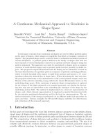
x
d
x
1, ,d−1
Figure 4: A linear velocity profile produces a pure horizontal shear stress.
equations which describe the transport of fluid material. Here, viscosity describes the internal
resistance in a fluid and may be thought of as a macroscopic measure of the friction between
fluid particles. As an example, the viscosity of honey is significantly larger than that of
water. Mathematically, the friction is described in terms of the stress tensor σ = (σ
ij
)
ij=1, d
,
whose entries describe a force per area element. By definition, σ
ij
is the force component
along the ith coordinate direction acting on the area element with a normal pointing in the
jth coordinate direction. Hence, the diagonal entries of the stress tensor σ refer to normal
stresses, e. g. due to compression, and the off-diagonal entries represent tangential (shear)

stresses. The Cauchy stress law states that due to the preservation of angular momentum
the stress tensor σ is symmetric [13].
In a Newtonian fluid the stress tensor is assumed to depend linearly on the gradient Dv
of the velocity v. In case of a rigid body motion the stress vanishes. A rotational component
of the local motion is generated by the antisymmetric part
1
2
(Dv − (Dv)
T
) of the velocity
gradient Dv := (
∂v
i
∂x
j
)
ij=1, d
, and it has the local rotation axis ∇ × v and local angular
velocity |∇×v| [40]. Hence, as rotations are rigid body motions, the stress only depends on
the symmetric part [v] :=
1
2
(Dv+(Dv)
T
) of the velocity gradient. If we separate compressive
stresses, reflected by the trace of the velocity gradient, from shear stresses depending solely
on the trace-free part of the velocity gradient, we obtain the constitutive relation of an
isotropic Newtonian fluid,
σ
ij

= µ (σ
shear
)
ij
+ K
c
(σ
bulk
)
ij
:= µ

∂v
i
∂x
j
+
∂v
j
∂x
i
−
2
d

k
∂v
k
∂x
k

δ
ij

+ K
c

k
∂v
k
∂x
k
δ
ij
, (2)
where µ is the viscosity, K
c
is the modulus of compression, and δ
ij
is the Kronecker symbol.
The following simple configuration serves for illustration. We consider a fluid volume
in R
d
, enclosed between two parallel plates at height 0 and H, where the vertical direction
normal to the two plates points along the x
d
-coordinate (cf. Fig. 4). Let us assume the lower
plate to be fixed and the upper plate to move horizontally at speed v
∂
= (v
∂

1
, ··· , v
∂
d−1
, 0).
Then, the velocity field v(x) =
x
d
H
v
∂
is a motion field consistent with the boundary conditions,
and the resulting stress is the pure shear stress µ
v
∂
H
, acting on all area elements parallel to
the two planes.
Introducing λ := K
c
−
2µ
d
and denoting the jth entry of the ith row of  by 
ij
, one can
rewrite (2) as
σ
ij
= λδ

ij

k

kk
+ 2µ
ij
,
or in matrix notation σ = λtr() + 2µ, where is the identity matrix and  = [v]. The
parameter λ is denoted Lam´e’s first coefficient. The local rate of viscous dissipation—the
rate at which mechanical energy is locally converted into heat due to friction—can now be
5
computed as
diss[v] =
λ
2
(tr[v])
2
+ µtr([v]
2
)
=
λ
2

d

i=1
v
i,i


2
+ µ
d

i,j=1
(v
i,j
+ v
j,i
)
2
4
, (3)
where we abbreviated v
i,j
=
∂v
i
∂x
j
. To see this, note that by its mechanical definition, the
stress tensor σ is the first variation of the local dissipation rate with respect to the velocity
gradient, i. e. σ = δ
Dv
diss . Indeed, by a straightforward computation we obtain
δ
(Dv)
ij
diss = λ tr δ

ij
+ 2µ 
ij
= σ
ij
.
If each point of the object O(t) at time t ∈ [0, 1] moves at the velocity v(x, t) so that the
total deformation of O(0) into O(t) can be obtained by integrating the velocity field v in
time, then the accumulated global dissipation of the motion field v in the time interval [0, 1]
takes the form
Diss

(v(t), O(t))
t∈[0,1]

=

1
0

O(t)
diss[v] dx dt . (4)
Here tr([v]
2
) measures the averaged local change of length and (tr[v])
2
the local change of
volume induced by the transport. Obviously div v = tr([v]) = 0 characterizes an incom-
pressible fluid.
Unlike in elasticity models (where the forces on the material depend on the original

configuration) or plasticity models (where the forces depend on the history of the flow),
in the Newtonian model of viscous fluids the rate of dissipation and the induced stresses
solely depend on the gradient of the motion field v in the above fashion. Even though the
dissipation functional (4) looks like the deformation energy from linearized elasticity, if the
velocity is replaced by the displacement, the underlying physics is only related in the sense
that an infinitisimal displacement in the fluid leads to stresses caused by viscous friction,
and these stresses are immediately absorbed via dissipation, which reflects a local heating.
In this paper we address the problem of computing geodesic paths and distances between
non-rigid shapes. Shapes will be modeled as the boundary contour of a physical object that
is made of a viscous fluid. The fluid flows according to a motion field v, where there is no flow
outside the object boundary. The external forces which induce the flow can be thought of
as originating from the dissimilarity between consecutive shapes. The resulting Riemannian
metric on the shape space, which defines the distance between shapes, will then be identified
with the rate of dissipation, representing the rate at which mechanical energy is converted
into heat due to the fluid friction whenever a shape is deformed into another one.
1.2 Related work on shape distances and geodesics
Conceptually, in the last decade, the distance between shapes has been extensively studied
on the basis of a general framework of the space of shapes and its intrinsic structure. The
notion of a shape space has been introduced already in 1984 by Kendall [25]. We will now
discuss related work on measuring distances between shapes and geodesics in shape space,
6
particularly emphasizing the relation to the above concepts from continuum mechanics.
An isometrically invariant distance measure between two objects S
A
and S
B
in (different)
metric spaces is the Gromov–Hausdorff distance [23], which is (in a simplified form) defined
as the minimizer of
1

2
sup
y
i
=φ(x
i
),ψ(y
i
)=x
i
|d(x
1
, x
2
) −d(y
1
, y
2
)| over all maps φ : S
A
→ S
B
and
ψ : S
B
→ S
A
, matching point pairs (x
1
, x

2
) in S
A
with pairs (y
1
, y
2
) in S
B
. It evaluates—
globally and based on an L
∞
-type functional—the lack of isometry between two different
shapes. M´emoli and Sapiro [31] introduced this concept into the shape analysis community
and discussed efficient numerical algorithms based on a robust notion of intrinsic distances
d(·, ·) on shapes given by point clouds. Bronstein et al. incorporate the Gromov–Hausdorff
distance concept in various classification and modeling approaches in geometry processing [7].
In [30] Manay et al. define shape distances via integral invariants of shapes and demon-
strate the robustness of this approach with respect to noise.
Charpiat et al. [10] discuss shape averaging and shape statistics based on the notion of
the Hausdorff distance and on the H
1
-norm of the difference of the signed distance functions
of shapes. They study gradient flows for energies defined as functions over these distances
for the warping between two shapes. As the underlying metric they use a weighted L
2
-
metric, which weights translational, rotational, and scale components differently from the
component in the orthogonal complement of all these transforms. The approach by Eckstein
et al. [19] is conceptually related. They consider a regularized geometric gradient flow for

the warping of surfaces.
When warping objects bounded by shapes in R
d
, a shape tube in R
d+1
is formed. Delfour
and Zol´esio [15] rigorously develop the notion of a Courant metric in this context. A further
generalization to classes of non-smooth shapes and the derivation of the Euler–Lagrange
equations for a geodesic in terms of a shortest shape tube is investigated by Zol´esio in [48].
There is a variety of approaches which consider shape space as an infinite-dimensional
Riemannian manifold. Michor and Mumford [32] gave a corresponding definition exempli-
fied in the case of planar curves. Yezzi and Mennucci [43] investigated the problem that
a standard L
2
-metric on the space of curves leads to a trivial geometric structure. They
showed how this problem can be resolved taking into account the conformal factor in the
metric. In [33] Michor et al. discuss a specific metric on planar curves, for which geodesics
can be described explicitly. In particular, they demonstrate that the sectional curvature on
the underlying shape space is bounded from below by zero which points out a close relation
to conjugate points in shape space and thus to only locally shortest geodesics. Younes [44]
considered a left-invariant Riemannian distance between planar curves. Miller and Younes
generalized this concept to the space of images [34]. Klassen and Srivastava [27] proposed
a framework for geodesics in the space of arclength parametrized curves and suggested a
shooting-type algorithm for the computation whereas Schmidt et al. [37] presented an alter-
native variational approach.
Dupuis et al. [18] and Miller et al. [35] defined the distance between shapes based on a
flow formulation in the embedding space. They exploited the fact that in case of sufficient
Sobelev regularity for the motion field v on the whole surrounding domain Ω, the induced
flow consists of a family of diffeomorphisms. This regularity is ensured by a functional


1
0

Ω
Lv ·v dx dt, where L is a higher order elliptic operator [39, 44]. Thus, if one considers
the computational domain Ω to contain a homogeneous isotropic fluid, then Lv ·v plays the
role of the local rate of dissipation in a multipolar fluid model [36], which is characterized by
the fact that the stresses depend on higher spatial derivatives of the velocity. Geometrically,

Ω
Lv · v dx is the underlying Riemannian metric. If L acts only on [v] and is symmetric,
7
then following the arguments in Section 1.1, rigid body motion invariance is incorporated
in this multipolar fluid model. Different from this approach we conceptually measure the
rate of dissipation only on the evolving object domain, and our model relies on classical
(monopolar) material laws from fluid mechanics not involving higher order elliptic operators.
Under sufficient smoothness assumptions Beg et al. derived the Euler–Lagrange equations
for the diffeomorphic flow field in [4]. To compute geodesics between hypersurfaces in the
flow of diffeomorphism framework, a penalty functional measures the distance between the
transported initial shape and the given end shape. Vaillant and Glaun`es [41] identified
hypersurfaces with naturally associated two forms and used the Hilbert space structures
on the space of these forms to define a mismatch functional. The case of planar curves is
investigated under the same perspective by Glaun`es et al. in [22]. To enable the statistical
analysis of shape structures, parallel transport along geodesics is proposed by Younes et
al. [45] as the suitable tool to transfer structural information from subject-dependent shape
representations to a single template shape.
In most applications, shapes are boundary contours of physical objects. Fletcher and
Whitaker [20] adopt this view point to develop a model for geodesics in shape space which
avoids overfolding. Fuchs et al. [21] propose a Riemannian metric on a space of shape
contours motivated by linearized elasticity, leading to the same quadratic form (1) as in

our approach, which is in their case directly evaluated on a displacement field between two
consecutive objects from a discrete object path. They use a B-spline parametrization of
the shape contour together with a finite element approximation for the displacements on
a triangulation of one of the two objects, which is transported along the path. Due to
the built-in linearization already in the time-discrete problem this approach is not strictly
rigid body motion invariant, and interior self-penetration might occur. Furthermore, the
explicitly parametrized shapes on a geodesic path share the same topology, and contrary to
our approach a cascadic relaxation method is not considered.
A Riemannian metric in the space of 3D surface triangulations of fixed mesh topology
has been investigated by Kilian et al. [26]. They use an inner product on time-discrete
displacement fields to measure the local distance from a rigid body motion. These local
defect measures can be considered as a geometrically discrete rate of dissipation. Mainly
tangential displacements are taken into account in this model. Spatially discrete and in the
limit time-continuous geodesic paths are computed in the space of discrete surfaces with a
fixed underlying simplicial complex. Recently, Liu et al. [28] used a discrete exterior calculus
approach on simplicial complexes to compute geodesics and geodesic distances in the space
of triangulated shapes, in particular taking care of higher genus surfaces.
1.3 Key contributions
The main contributions of our approach are the following:
• A direct connection between physics-motivated and geometry-motivated shape spaces
is provided, and an intuitive physical interpretation is given based on the notion of
viscous dissipation.
• The approach mathematically links a pairwise matching of consecutive shapes and
a viscous flow perspective for shapes being boundary contours of objects which are
represented by possibly multi-labeled images. The time discretization of a geodesic
8
path based on this pairwise matching ensures rigid body motion invariance and a 1-1
mapping property.
• The implicit treatment of shapes via level sets allows for topological transitions and
enables the computation of geodesics in the context of partial occlusion. Robustness

and effectiveness of the developed algorithm are ensured via a cascadic multi–scale
relaxation strategy.
2 The variational formulation
Within this section, in 2.1 we put forward a model of discrete geodesics as a finite number
of shapes S
k
, k = 0, . . . , K, connected by deformations φ
k
: O
k−1
→ R
d
which are optimal
in a variational sense and fulfill the hard constraint φ
k
(S
k−1
) = S
k
. Subsequently, in 2.3
we relax this constraint using a penalty formulation. Afterwards, based on a viscous fluid
formulation, in 2.4 we introduce a model for geodesics that are continuous in time, and in
2.5 we finally show that the latter model is obtained from the time-discrete model in the
limit for vanishing time step size.
2.1 The time-discrete geodesic model
As already outlined above we do not consider a purely geometric notion of shapes as curves
in 2D or surfaces in 3D. In fact, motivated by physics, we consider shapes S as boundaries
∂O of sufficiently regular, open object domains O ⊂ R
d
for d = 2, 3. Let us denote by S a

suitable admissible set of such shapes - the actual shape space. Later, in Section 4.2, this
set will be generalized for shapes in the context of multi-labeled images.
Given two shapes S
A
, S
B
in S, we define a discrete path of shapes as a sequence of shapes
S
0
, S
1
, . . . , S
K
⊂ S with S
0
= S
A
and S
K
= S
B
. For the time step τ =
1
K
the shape S
k
is supposed to be an approximation of S(t
k
) for t
k

= kτ, where (S(t))
t∈[0,1]
is a continuous
path connecting S
A
= S(0) and S
B
= S(1).
Now, we consider a matching deformation φ
k
: O
k−1
→ R
d
for each pair of consecutive
shapes S
k−1
and S
k
in a suitable admissible space of orientation preserving deformations
D[O
k−1
] and impose the constraint φ
k
(S
k−1
) = S
k
. With each deformation φ
k

we associate
a deformation energy
E
deform
[φ
k
, S
k−1
] =

O
k−1
W (Dφ
k
) dx , (5)
where W is an energy density which, if appropriately chosen, will ensure sufficient regularity
and a 1-1 matching property for a deformation φ
k
minimizing E
deform
over D[O
k−1
] under the
above constraint. Analogously to the axiom of elasticity, the energy is assumed to depend
only on the local deformation, reflected by the Jacobian Dφ := (
∂φ
i
∂x
j
)

ij=1, d
. Yet, different
from elasticity, we suppose the material to relax instantaneously so that object O
k
is again in
a stress-free configuration when applying φ
k+1
at the next time step. Let us also emphasize
that the stored energy does not depend on the deformation history as in most plasticity
models in engineering.
Given a discrete path, we can ask for a suitable measure of the time-discrete dissipation
accumulated along the path. Here, we identify this dissipation with a scaled sum of the
9
accumulated deformation energies E
deform
[φ
k
, S
k−1
] along the path. Furthermore, the inter-
pretation of the dissipation rate as a Riemannian metric motivates a corresponding notion
of an approximate length for any discrete path. This leads to the following definition:
Definition 1 (Discrete dissipation and discrete path length). Given a discrete path S
0
,
S
1
, . . ., S
K
∈ S, the total dissipation along a path can be computed as

Diss
τ
(S
0
, S
1
, . . . , S
K
) :=
K

k=1
1
τ
E
deform
[φ
k
, S
k−1
] ,
where φ
k
is a minimizer of the deformation energy E
deform
[·, S
k−1
] over D[O
k−1
] under the

constraint φ
k
(S
k−1
) = S
k
. Furthermore, the discrete path length is defined as
L
τ
(S
0
, S
1
, . . . , S
K
) :=
K

k=1

E
deform
[φ
k
, S
k−1
] .
Let us make a brief remark on the proper scaling factor for the time-discrete dissipation.
Indeed, the energy E
deform

[φ
k
, S
k−1
] is expected to scale like τ
2
. Hence, the factor
1
τ
ensures
a dissipation measure which is conceptually independent of the time step size. The same
holds for the discrete length measure

E
deform
[φ
k
, S
k−1
], which already scales like τ. Thus
L
τ
(S
0
, S
1
, . . . , S
K
) indeed reflects a path length. To ensure that the above-defined dissipa-
tion and length of discrete paths in shape space are well-defined, a minimizing deformation

φ
k
of the elastic energy E
deform
[·, S
k−1
] has to exist. In fact, this holds for objects O
k−1
and
O
k
with Lipschitz boundaries S
k−1
and S
k
for which there exists at least one bi-Lipschitz
deformation
ˆ
φ
k
from O
k−1
to O
k
for k = 1, . . . , K (i. e.
ˆ
φ
k
is Lipschitz and injective and has
a Lipschitz inverse). The associated class of admissible deformations will essentially consist

of those deformations with finite energy. Here, we postpone this discussion until the energy
density of the deformation energy is fully introduced.
With the notion of dissipation at hand we can define a discrete geodesic path following the
standard paradigms in differential geometry:
Definition 2 (Discrete geodesic path). A discrete path S
0
, S
1
, . . . , S
K
in a set of admissible
shapes S connecting two shapes S
A
and S
B
in S is a discrete geodesic if there exists an
associated family of deformations (φ
k
)
k=1, ,K
with φ
k
∈ D[O
k−1
] and φ
k
(S
k−1
) = S
k

such that
(φ
k
, S
k
)
k=1, ,K
minimize the total energy

K
k=1
E
deform
[
˜
φ
k
,
˜
S
k−1
] over all intermediate shapes
˜
S
1
, . . . ,
˜
S
K−1
∈ S and all possible matching deformations

˜
φ
1
, . . . ,
˜
φ
K
with
˜
φ
k
∈ D[
˜
O
k−1
],
˜
S
k−1
= ∂
˜
O
k−1
, and
˜
φ
k
(
˜
S

k−1
) =
˜
S
k
for k = 1, . . . , K.
In the following, we will inspect an appropriate model for the deformation energy density
W . As a fundamental requirement for the time discretization we postulate the invariance of
the deformation energy with respect to rigid body motions, i. e.
E
deform
[Q ◦φ
k
+ b, S
k−1
] = E
deform
[φ
k
, S
k−1
] (6)
for any orthogonal matrix Q ∈ SO(d) and b ∈ R
d
(the axiom of frame indifference in con-
tinuum mechanics). From this one deduces that the energy density only depends on the
right Cauchy–Green deformation tensor Dφ
T
Dφ, i. e. there is a function
¯

W : R
d,d
→ R such
that the energy density W satisfies W (F ) =
¯
W (F
T
F ) for all F ∈ R
d,d
. Indeed, if (6) holds
10
for arbitrary S
k−1
, φ
k
, and Q ∈ SO(d), then we have to have W(QF) = W (F ) for any
Q ∈ SO(d) and any orientation preserving matrix F ∈ R
d,d
(in particular, F = Dφ
k
(x) for
any x ∈ O
k−1
). By the polar decomposition theorem, we can decompose such an F into
the product of an orthogonal matrix Q ∈ SO(d) and a symmetric positive definite matrix C
with C =
√
F
T
F and Q = F

√
F
T
F
−1
. Thus, W(F ) = W(Q
√
F
T
F ) = W (
√
F
T
F ) so that
W (F ) can indeed be rewritten as
¯
W (F
T
F ), where
¯
W (C) := W (
√
C) for positive definite
matrices C ∈ R
d,d
.
The Cauchy–Green deformation tensor geometrically represents the metric measuring the
deformed length in the undeformed reference configuration.
For an isotropic material and for d = 3 the energy density can be further rewritten as a func-
tion

ˆ
W (I
1
, I
2
, I
3
) solely depending on the principal invariants of the Cauchy–Green tensor,
namely I
1
= tr(Dφ
T
Dφ), controlling the local average change of length, I
2
= tr(cof(Dφ
T
Dφ))
(cofA := det A A
−T
), reflecting the local average change of area, and I
3
= det (Dφ
T
Dφ),
which controls the local change of volume. For a detailed discussion we refer to [14, 40]. Let
us remark that tr(A
T
A) coincides with the Frobenius norm |A| of the matrix A ∈ R
d,d
and

the corresponding inner product on matrices is given by A : B = tr(A
T
B). Furthermore, let
us assume that the energy density is a convex function of Dφ, cofDφ, and det Dφ, and that
isometries, i. e. deformations with Dφ
T
(x)Dφ(x) = , are global minimizers [14]. For the
impact of this assumption on the time discrete geodesic application we refer in particular to
the second row in Fig. 5, which provides an example of striking global isometry preservation
and an only local lack of isometry. We may further assume W ( ) =
ˆ
W (d, d, 1) = 0 without
any restriction. An example of this class of energy densities is
ˆ
W (I
1
, I
2
, I
3
) = α
1
I
p
2
1
+ α
2
I
q

2
2
+ Γ(I
3
) (7)
with p > 1, q ≥ 1, α
1
> 0, α
2
≥ 0, and Γ convex with Γ(I
3
) → ∞ for I
3
→ 0 or I
3
→ ∞,
where the parameters are chosen such that (I
1
, I
2
, I
3
) = (d, d, 1) is the global minimizer (cf.
the concrete energy density defined in Appendix A.1) . The built-in penalization of volume
shrinkage, i. e.
¯
W
I
3
→0

−→ ∞, comes along with a local injectivity result [3]. Thus, the sequence
of deformations φ
k
linking objects O
k−1
and O
k
actually represents homeomorphisms (which
for deformations with finite energy is rigorously proved under mild assumptions such as
sufficiently large p, q, certain growth conditions on Γ, and the objects embedded in a very
soft instead of void material for which Dirichlet boundary conditions are prescribed). We
refer to [16], where a similar energy has been used in the context of morphological image
matching. Let us remark that in case of a void background, self-contact at the boundary
is still possible so that the mapping from S
k−1
= ∂O
k−1
to S
k
= ∂O
k
does not have to be
homeomorphic. With the interpretation of such self-contact as a closing of the gap between
two object boundaries in the sense that the viscous material flows together, our model allows
for topological transitions along a discrete path in shape space [14] (cf. the geodesic from
the letter A to the letter B in Fig. 1 for an example).
2.2 An existence result for the time-discrete model
Based on these mechanical preliminaries we can now state an existence result for discrete
geodesic paths for a suitable choice of the admissible set of shapes S and corresponding
function spaces D[O

k
] for the deformations φ
k
, k = 1, . . . , K. Note that the known regularity
theory in nonlinear elasticity [3, 12] does not allow to control the Lipschitz regularity of the
11
deformed boundary φ
k
(S
k−1
) even if S
k−1
is a Lipschitz boundary of the elastic domain O
k−1
.
One way to obtain a well-posed formulation of the whole sequence of consecutive variational
problems for the deformations φ
k
and shapes S
k
is to incorporate the required regularity
of the shapes in the definition of the shape space. Hence, let us assume that S consists of
shapes S which are boundary contours of open, bounded sets O and can be decomposed
into a bounded number of spline surfaces with control points on a fixed compact domain.
Furthermore, the shapes are supposed to fulfill a uniform cone condition, i. e. each point
x ∈ S is the tip of two open cones with fixed opening angle α > 0 and height r > 0,
one contained in the domain O and the other in the complement of O. On such object
domains, the variational problem for a single deformation φ
k
connecting shapes S

k−1
and S
k
can be solved based on the direct method of the calculus of variations. With regard to the
deformation energy integrand in (7), the natural function space for the deformations φ
k
is a
subset of the Sobolev space W
1,p
(O
k−1
) [1]. Let us take into account an explicit function Γ,
namely the rational function Γ(I
3
) = α
3

I
−
s
2
3
+ βI
r
2
3

− γ. Then, in d = 3 dimensions, for
α
1

, α
2
, α
3
, β, γ > 0, p, q > 3, r > 1 and s >
2q
q−3
, we choose
D[O
k−1
] := {φ : O
k−1
→ R
d


φ ∈ W
1,p
(O
k−1
), cofDφ ∈ L
q
(O
k−1
),
det Dφ ∈ L
r
(O
k−1
), det Dφ > 0 a.e. in O

k−1
, φ(O
k−1
) = O
k
}.
Taking into account this space of admissible deformations for each k ∈ {1, . . . , K} leads to
a well-defined notion of dissipation and length for discrete paths:
Theorem 1 (Existence of a discrete geodesic). Given two diffeomorphic shapes S
A
and S
B
in the above shape space S, there exists a discrete geodesic S
0
, S
1
, . . . , S
K
∈ S connecting
S
A
and S
B
. The associated deformations φ
1
, . . . , φ
K
with φ
k
∈ D[O

k−1
] for k = 1, . . . , K are
H¨older continuous (that is, |φ(x) − φ(y)| ≤ |x − y|
γ
for some γ ∈ (0, 1) and all points x, y)
and locally injective in the sense that the determinant of the deformation gradient is positive
almost everywhere.
Proof: To prove the existence of a discrete geodesic we make use of a nowadays classical
result from the vector-valued calculus of variations. Indeed, applying the existence results
for elastic deformations by Ball [2, 3], any pair of consecutive shapes S
k−1
and S
k
is as-
sociated with a H¨older continuous deformation φ
k
∈ D[O
k−1
] with det Dφ
k
> 0 almost
everywhere, which minimizes the deformation energy E
deform
[·, S
k−1
] among all deformations
φ ∈ D[O
k−1
]. Hence, given the set (φ
k

)
k=1, ,K
of such minimizing deformations for fixed
shapes S
1
, . . . , S
K
, we can compute the discrete dissipation
1
τ

K
k=1
E
deform
[φ
k
, S
k−1
] along the
discrete path S
1
, . . . , S
K
.
Now, we make use of the structural assumption on the shape space S. The space of all
shapes can be parametrized with finitely many parameters, namely the control points of the
spline segments. These control points lie in a compact set. Also, S is closed with respect to
the convergence of this set of parameters since the cone condition is preserved in the limit
for a convergent sequence of spline parameters.

To prove that a minimizer S
1
, . . . , S
K
of the discrete dissipation Diss
τ
exists, we first observe
that Diss
τ
effectively is a function of the finite set of spline parameters. Furthermore, the
set of admissible spline parameters is compact. Hence, it is sufficient to verify that Diss
τ
is continuous. For this purpose, consider shapes S
k−1
, S
k
and
˜
S
k−1
,
˜
S
k
, respectively. Fur-
thermore, for a given small δ
0
> 0 we can assume the spline parameters of (S
k−1
, S

k
) and
(
˜
S
k−1
,
˜
S
k
) to be close enough to each other so that for i = k − 1, k there exists a bijective
12
deformation ψ
i
:
˜
O
i
→ O
i
which is Lipschitz-continuous and has a Lipschitz-continuous
inverse ψ
−1
i
with |ψ
i
− |
1,∞
+



ψ
−1
i
−


1,∞
≤ δ for a δ ≤ δ
0
. Let us denote by φ,
˜
φ the
optimal deformations associated with the dissipation Diss
τ
(S
k−1
, S
k
) and Diss
τ
(
˜
S
k−1
,
˜
S
k
),

respectively. Using the optimality of
˜
φ and defining
ˆ
φ := ψ
−1
k
◦ φ ◦ψ
k−1
we can estimate
Diss
τ
(
˜
S
k−1
,
˜
S
k
)−Diss
τ
(S
k−1
, S
k
) =
1
τ


˜
O
k−1
W (D
˜
φ) dx −
1
τ

O
k−1
W (Dφ) dx
≤
1
τ

˜
O
k−1
W (D
ˆ
φ) dx −
1
τ

O
k−1
W (Dφ) dx
=
1

τ

O
k−1
W

(Dψ
−1
k
◦φ)Dφ(Dψ
k−1
◦ψ
−1
k−1
)

|det Dψ
−1
k−1
| −W(Dφ) dx .
Here, we have applied the chain rule and a change of variables. Taking into account the
explicit form of the integrand and the above assumption on ψ
k−1
and ψ
k
, we can estimate
the integrand from above independently of δ by
C(δ
0
)


|Dφ|
p
+ |cofDφ|
q
+ |det Dφ|
r
+


(det Dφ)
−1


s

,
where C(δ
0
) is a constant solely depending on δ
0
. Obviously, this pointwise bound itself is
integrable for φ ∈ D(O
k−1
). Thus, as we let δ → 0, from Lebesgue’s theorem we deduce that
Diss
τ
(
˜
S

k−1
,
˜
S
k
) −Diss
τ
(S
k−1
, S
k
) ≤ c(δ)
for a function c : R
+
→ R with lim
δ→0
c(δ) = 0. Exchanging the role of
˜
S
k−1
,
˜
S
k
and S
k−1
, S
k
we obtain
Diss

τ
(S
k−1
, S
k
) −Diss
τ
(
˜
S
k−1
,
˜
S
k
) ≤ c(δ)
which proves the required continuity of the dissipation Diss
τ
. Hence, there is indeed a dis-
crete geodesic S
0
, . . . , S
K
. 
2.3 A relaxed formulation
Computationally, the constraint φ
k
(S
k−1
) = S

k
for a 1-1 matching of consecutive shapes is
difficult to treat. Furthermore, the constraint is not robust with respect to noise. Indeed,
high frequency perturbations of the input shapes S
A
and S
B
might require high deformation
energies in order to map S
A
onto a regular intermediate shape or to obtain S
B
as the image
of a regular intermediate shape in a 1-1 manner. Hence, we ask for a relaxed formulation
which allows for an effective numerical implementation and is robust with respect to noisy
geometries. At first, we assume that the complement of the object O
k−1
also is deformable,
but several orders of magnitude softer than the object itself. Hence, we define
E
δ
deform
[φ
k
, S
k−1
] =

Ω


(1 −δ)χ
O
k−1
+ δ

W (Dφ
k
) dx (8)
13
Figure 5: Discrete geodesic for two different examples from [21] and [11] where the local
rate of dissipation is color-coded as . In the bottom example the local preservation of
isometries is clearly visible, whereas in the top example stretching is the major effect.
for deformations φ
k
now defined on a sufficiently large computational domain Ω. For simplic-
ity we assume φ
k
(x) = x on the boundary ∂Ω. This renders the subproblem of computing
an optimal elastic deformation well-posed independent of the current shape. For δ = 0, we
obtain the original model and suppose that at least a sufficiently smooth extension of the
deformation on a neighborhood of the shape is given.
Now, we are in the position to introduce a relaxed formulation of the pairwise matching
problem by adding a mismatch penalty
E
match
[φ
k
, S
k−1
, S

k
] = vol(O
k−1
φ
−1
k
(O
k
)) , (9)
where AB = A\B ∪B \A defines the symmetric difference between two sets and vol(A) =

A
dx is the d-dimensional volume of the set A. This mismatch penalty replaces the hard
matching constraint φ
k
(S
k−1
) = S
k
. Alternatively, one might consider the mismatch penalty
vol(φ
k
(O
k−1
)O
k
), but as we will see in Section 3.1, the form (9) is computationally more
feasible in case of an implicit shape description.
Next, in practical applications shapes are frequently defined as contours in images and usually
not given in explicit parametrized form. Hence, the restriction of the set of admissible shapes

to piecewise parametric shapes, which we have taken into account in the previous section
to establish an existence result for geodesic paths, is—from a computational viewpoint—not
very appropriate either. If we allow for more general shapes being boundary contours of
objects in images, one should at least require them to have a finite perimeter. Otherwise
it would be appropriate to decompose the initial object O
A
into tiny disconnected pieces,
shuffle these around via rigid body motions (at no cost), and remerge them to obtain the
final object O
B
. The property of finite perimeter can be enforced for the intermediate shapes
by adding the object perimeter (generalized surface area in d dimensions) as an additional
energy term
E
area
[S] =

S
da .
Finally, we obtain the following relaxed definition of a path functional for a family of defor-
mations and shapes:
14
Figure 6: Geodesic paths between an X and an M, without a contour length term (ν = 0, top
row), allowing for crack formation (marked by the arrows), and with this term damping down
cracks and rounding corners (bottom rows). In the bottom rows we additionally enforced
area preservation along the geodesic.
Definition 3 (Relaxed discrete path functional). Given a sequence of shapes (S
k
)
k=0, ,K

and
a family of deformations (φ
k
)
k=1, ,K
with φ
k
: O
k−1
→ R
d
we define the relaxed dissipation
as
E
δ
τ
[(φ
k
, S
k
)
k=1, ,K
] :=
K

k=1

E
δ
deform

[φ
k
, S
k−1
]
τ
+ η E
match
[φ
k
, S
k−1
, S
k
] + ν τ E
area
[S
k
]

, (10)
where η, ν are parameters. A minimizer of this energy defines a relaxed discrete geodesic
path between the shapes S
A
= S
0
and S
B
= S
K

.
As we will see in Section 2.5 below, the different scaling of the three energy components
with respect to the time step size τ will ensure a meaningful limit for τ → 0.
Fig. 6 shows an example of two different geodesics between the letters X and M, demon-
strating the impact of the term E
area
controlling the (d −1)-dimensional area of the shapes.
2.4 The time-continuous viscous fluid model
In this section we discuss geodesics in shape space from a Riemannian perspective and
elaborate on the relation to viscous fluids. This prepares the identification of the resulting
model as the limit of our time discrete formulations in the following section. A Riemannian
metric G on a differential manifold M is a bilinear mapping that assigns each element S ∈ M
an inner product on variations δS of S. The associated length of a tangent vector δS is given
by δS =

G(δS, δS). The length of a differentiable curve S : [0, 1] → M is then defined
by
L[S] =

1
0

˙
S(t)dt =

1
0

G(
˙

S(t),
˙
S(t)) dt ,
where
˙
S(t) is the temporal variation of S at time t. The Riemannian distance between two
points S
A
and S
B
on M is given as the minimal length taken over all curves with S(0) = S
A
and S(1) = S
B
. Hence, the shortest such curve S : [0, 1] → M is the minimizer of the length
functional L[S]. It is well-known from differential geometry that it is at the same time a
minimizer of the cost functional

1
0
G(
˙
S(t),
˙
S(t)) dt
15
and describes a geodesic between S
A
and S
B

of minimum length. Let us emphasize that
a general geodesic is only locally the shortest curve. In particular there might be multiple
geodesics of different length connecting the same end points.
In our case the Riemannian manifold M is the space of all shapes S in an admissible class of
shapes S (e. g. the one introduced in Section 2.1) equipped with a metric G on infinitesimal
shape variations. As already pointed out above, we consider shapes S as boundary contours
of deforming objects O. Hence, an infinitesimal normal variation δS of a shape S = ∂O is
associated with a transport field v :
¯
O → R
d
. This transport field is obviously not unique.
Indeed, given any vector field w on
¯
O with w(x) ∈ T
x
S for all x ∈ S = ∂O (where T
x
S
denotes the (d −1)-dimensional tangent space to S at x), the transport field v +w is another
possible representation of the shape variation δS. Let us denote by V(δS) the affine space
of all these representations. As a geometric condition for v ∈ V(δS) we obtain v ·n[S] = δS,
where n[S] denotes the outer normal of S. Given all possible representations we are interested
in the optimal transport, i. e. the transport leading to the least dissipation. Thus, using the
definition (1) of the local dissipation rate diss[v] =
λ
2
(tr[v])
2
+ µ tr([v]

2
) we define the
metric G(δS, δS) as the minimal dissipation on motion fields v, which are consistent with
the variation of the shape δS:
G(δS, δS) := min
v∈V(δS)

O
diss[v] dx = min
v∈V(δS)

O
λ
2
(tr[v])
2
+ µ tr([v]
2
) dx . (11)
Let us remark that we distinguish explicitly between the metric g(v, v) :=

O
diss[v] dx on
motion fields and the metric G(δS, δS) on (the different space of) shape variations, which
is the minimum of g(v, v) over all motion fields consistent with δS. Finally, integration in
time leads to the total dissipation
min
v(t)∈V(
˙
S(t))

Diss

(v(t), O(t))
t∈[0,1]

=

1
0
G(
˙
S(t),
˙
S(t)) dt
to be invested in the transport along a path (S(t))
t∈[0,1]
in the shape space S. This implies
the following definition of a time continuous geodesic path in shape shape:
Definition 4 (Time-continuous geodesic path). Given two shapes S
A
and S
B
in a shape
space S, a geodesic path between S
A
and S
B
is a curve (S(t))
t∈[0,1]
⊂ S with S(0) = S

A
and
S(1) = S
B
which is a local solution of
min
v(t)∈V(
˙
S(t))
Diss

(v(t), O(t))
t∈[0,1]

among all differentiable paths in S.
Evidently, one has to minimize over all motion fields v in space and time which are
consistent with the temporal evolution of the shape. As in the time-discrete case, we can relax
this property and consider general vector fields v which are defined at time t on the domain
¯
O(t) but are not necessarily consistent with the evolving shape. The lack of consistency is
instead penalized via the functional
E
OF
[(v(t), S(t))
t∈[0,1]
] =

T
|(1, v(t)) · n[t, S(t)]| da , (12)
16

where (1, v(t)) is the underlying space-time motion field and n[t, S(t)] the space-time normal
on the shape tube T :=

t∈[0,1]
(t, S(t)) ⊂ [0, 1] ×R
d
. If we denote by χ
T
O
the characteristic
function of the associated (d+1)-dimensional domain tube T
O
:=

t∈[0,1]
(t, O(t)) on [0, 1]×R
d
then—with a slight misuse of notation—we can rewrite this functional as
E
OF
[(v(t), S(t))
t∈[0,1]
] =

(0,1)×R
d


∂
t

χ
T
O
+ ∇
x
χ
T
O
· v


dx dt . (13)
Obviously, there is a similarity to TV-type variational approaches in optical flow [5], where
v is the optical flow field and (t, x) → χ
O(t)
(x) is the intensity map of the corresponding
image sequence.
Additionally, we may consider a further regularization term on the tube of shapes, which
integrates the surface area E
area
[S(t)] =

S(t)
da over time so that we finally obtain the
time-continuous path functional
E[(v(t), S(t))
t∈[0,1]
] =

1

0

O(t)
diss[v] dx dt+η E
OF
[(v(t), S(t))
t∈[0,1]
]+ν

1
0

S(t)
da dt . (14)
Let us remark that the second and the third energy term can be considered as anisotropic
measures of area on the space-time tube T . Indeed, the last term integrates the (d − 1)-
dimensional area on cross sections of T whereas the second term weights the area element
|∇
(t,x)
χ
T
O
| with the space time motion field (1, v).
2.5 The viscous fluid model as a limit for τ → 0
We now investigate the relation of the above-introduced relaxed discrete geodesic paths and
the time continuous model for geodesics in shape space. For this purpose, we choose the
deformation energy in such a way that the Hessian of the energy E
deform
with respect to the
deformation of an object O, evaluated at the identity deformation , coincides up to a factor

1
2
with the dissipation rate or metric tensor based on (1), i. e.
Hess E
deform
[ , S](v, v) = 2

O
diss[v] dx (15)
for any velocity field v. In terms of the energy density W this is expressed by the condition
d
2
dt
2
W ( + tA)|
t=0
= λ(trA)
2
+
µ
2
tr


A + A
T

2

(16)

for the second derivative of W . By straightforward computation one verifies that for any
local dissipation rate (1) one can find a nonlinear energy density of type (7) which satisfies
(16). This is detailed in Appendix A.1, expressing the free parameters of the deformation
energy density (7) in terms of the dissipation parameters λ and µ.
Next, let us introduce the following notation. Given a sequence S
0
, . . . , S
K
of shapes and
deformations φ
1
, . . . , φ
K
with φ
k
being defined on O
k−1
, we introduce a temporally piecewise
constant motion field v
k
τ
and a time-continuous deformation field φ
k
τ
(which interpolates
17
between points x ∈ O
k−1
and φ
k

(x) ∈ O
k
) by
v
k
τ
(t) :=
1
τ
(φ
k
− ) ,
φ
k
τ
(t) := ( + (t − t
k−1
)v
k
τ
)
for t ∈ [t
k−1
, t
k
) with t
k
= kτ . The corresponding Eulerian motion field, which actually
generates the flow, is then given by
v

τ
(t) := v
k
τ
◦ (φ
k
τ
)
−1
.
Here, we assume that φ
k
τ
is injective.The concatenation with its inverse is only needed to
obtain the proper Eulerian description of the motion field.
For decreasing time step size τ , we are interested in the behavior of the total energy
E
0
τ
on families of deformations and shapes, given by the time-discrete, relaxed model from
Definition 3, and its relation to the energy E on motion fields and shapes in space-time
introduced in Definition 4. In fact, if we evaluate the energy E
0
τ
on a family of deformations
and shapes, where the deformations are induced by some smooth motion field v and the
shapes are obtained from a smooth shape tube T =

t∈[0,1]
(t, S(t)) via regular sampling, we

observe convergence to the time-continuous energy E evaluated on v and T as postulated in
the following theorem:
Theorem 2 (Limit functional for vanishing time step size). Let us assume that (S(t))
t∈[0,1]
is a smooth family of shapes and consider a time step size τ =
1
K
with K → ∞. For each
fixed value of K choose S
k
= S(kτ) for k = 0, . . . , K. Furthermore, let φ
1
, . . . , φ
K
be a
sequence of injective deformations with φ
k
being defined on
¯
O
k−1
. Finally, assume that the
associated motion field v
τ
converges for K → ∞ to a smooth motion field v on the space-time
tube

t∈[0,1]
(t,
¯

O(t)). Then the relaxed discrete path functional E
0
τ
[(φ
k
, S
k
)
k=1, ,K
] converges
to the time-continuous path functional E[(v(t), S(t))
t∈[0,1]
] for K → ∞.
We conclude that our variational time discretization is indeed consistent with the time-
continuous viscous dissipation model of geodesic paths. In particular, the length control
based on the first invariant I
1
of Dφ
k
turns into the control of infinitesimal length changes
via tr([v]
2
), and the control of volume changes based on the third invariant I
3
of Dφ
k
turns
into the control of compression via tr([v])
2
(cf. Fig. 7 for the impact of these two terms on

the shapes along a geodesic path). Note that our primal interest lies in the case η  1 since
the L
1
-type optical flow term is supposed to just act as a penalty.
Proof (Theorem 2): At first, let us investigate the convergence behavior of the sum of
deformation energies

K
k=1
1
τ
W[O
k−1
, φ
k
]. We consider a second order Taylor expansion
around the identity and obtain
W (Dφ
k
) = W ( ) + τW
,A
( )(Dv
k
τ
) +
τ
2
2
W
,AA

( )(Dv
k
τ
, Dv
k
τ
) + O(τ
3
)
= 0 + 0 +
τ
2
2
d
2
dt
2
W ( + tDv
k
τ
)|
t=0
+ O(τ
3
)
= τ
2

λ
2

(trDv
k
τ
)
2
+
µ
4
tr


Dv
k
τ
+ (Dv
k
τ
)
T

2


+ O(τ
3
)
= τ
2
diss[v
k

τ
] + O(τ
3
) .
18
Figure 7: Two geodesic paths between dumb bell shapes varying in the size of the ends. In
the top example the ratio λ/µ between the parameters of the dissipation is 0.01 (leading
to rather independent compression and expansion of the ends since the associated change
of volume implies relatively low dissipation), and 100 in the bottom example (now mass
is actually transported from one end to the other). The underlying texture on the shape
domains O
0
, . . . , O
K−1
is aligned to the transport direction, and the absolute value of the
velocity v is color-coded as .
Here, we have used that the identity deformation is the minimizer of W (·) with W( ) = 0
as well as the relation between W and diss from (16). Now, summing over all deformation
energy contributions yields
lim
K→∞
K

k=1
1
τ
E
deform
[φ
k

, S
k−1
] = lim
K→∞
K

k=1
1
τ

O
k−1
W (Dφ
k
) dx
= lim
K→∞
K

k=1
τ

O
k−1
diss[v
k
τ
] dx =

1

0

O(t)
diss[v] dx dt
so that we recover the viscous dissipation in the limit.
Next, we investigate the limit behavior of the sum of mismatch penalty functionals for
vanishing time step size. In a neighborhood of the shape S
k−1
, let us for x ∈ S
k−1
define the
local and signed thickness function (cf. Fig. 8)
δ
k
(x) := sup {s : φ
k
(x + sn[S
k−1
](x)) ∈ O
k
}
of the mismatch set O
k−1
φ
−1
k
(O
k
) (recall that φ
k

is extended outside O
k−1
). Then, we
obtain
vol(O
k−1
φ
−1
k
(O
k
)) =

S
k−1
|δ
k
(x)|da + o(τ) . (17)
Furthermore, we connect the shapes S
k−1
= S(t
k−1
) and S
k
= S(t
k
) via a ruled surface
T
ruled
k

: For x ∈ S
k−1
we suppose a vector r
k
(x) ∈ R
d
with r
k
= O(τ) to be defined by the
19
properties r
k
(x) ⊥ T
x
S
k−1
and x + r
k
(x) ∈ S
k
. Then define
T
ruled
k
:=

t, x +
t −t
k−1
τ

r
k
(x)

: t ∈ [t
k−1
, t
k
], x ∈ S
k−1

.
Obviously, T
ruled
k
approximates the continuous tube T
k
:= ∪
t
k−1
≤t≤t
k
(t, S(t)) up to terms of
the order O(τ
2
). We denote by n
k
[t
k−1
, S

k−1
](x) the normal vector on the ruled surface
T
ruled
k
at a point x ∈ S
k−1
. In particular, n
k
[t
k−1
, S
k−1
](x) ⊥ (0, w) ∀w ∈ T
x
S
k−1
and
n
k
[t
k−1
, S
k−1
](x) ⊥ (τ, r
k
(x)). From these properties we get that
|(τ, r
k
(x) −δ

k
(x)n[S
k−1
](x)) ·n
k
[t
k−1
, S
k−1
](x)| = τ |(1, v
k
τ
(x)) ·n
k
[t
k−1
, S
k−1
](x)| + o(τ) .(18)
Next, by an elementary geometric argument for
l
k
(x) :=

τ
2
+ |r
k
(x)|
2

,
ε
k
(x) := (τ, r
k
(x) −δ
k
(x)n[S
k−1
](x)) ·n
k
[t
k−1
, S
k−1
](x)
we obtain that
|δ
k
(x)|
|ε
k
(x)|
=
l
k
(x)
τ
and hence
|ε

k
(x)|l
k
(x)
τ
= |δ
k
(x)|.
Using this relation together with (18) and taking into account further standard approxima-
tion arguments we obtain

T
k
|(1, v(x)) · n[t, S(t)](x)|da =

T
ruled
k
|(1, v
k
τ
(x)) ·n
k
[t
k−1
, S
k−1
](x)|da + o(τ)
=


S
k−1
|(1, v
k
τ
(x)) ·n
k
[t
k−1
, S
k−1
](x)|l
k
(x) da + o(τ)
=

S
k−1
1
τ
|(τ, r
k
(x) −δ
k
(x)n[S
k−1
](x)) ·n
k
[t
k−1

, S
k−1
](x)|l
k
(x) da + o(τ)
=

S
k−1
|δ
k
(x)|da + o(τ)
so that by (17) we finally arrive at the desired result
vol(O
k−1
φ
−1
k
(O
k
)) =

T
k
|(1, v(x)) · n[t, S(t)](x)|da + o(τ) .
Finally, the sum of shape perimeters,

K
k=1
τE

area
[S
k
], obviously converges to the time integral
of the perimeters,

1
0

S(t)
da dt
so that we have verified the postulated convergence. 
Let us remark that we do not prove Γ-convergence of the relaxed discrete path functional as
the time step size approaches zero. Here, the issue of compactness of the family of shapes
and deformations with finite energy as well as the lower semi-continuity are open problems.
20
O
k−1
φ
−1
k
(O
k
)
O
k
S
k−1
φ
−1

k
(S
k
)
S
k
x
δ
k
(x)n[S
k−1
](x)
x + r
k
(x)
t
k−1
t
k
t
O
k−1
O
k
T
ruled
k
(t
k
, x)

δ
k
(x)n[S
k−1
](x)
r
k
(x)
l
k
(x)
|ε
k
(x)|
τ
x
Figure 8: Sketch of the mismatch between shapes and motion fields. The left sketch illus-
trates the quantities from the proof for a geodesic path of 2D shapes, and the middle shape
shows a close-up. The right graph shows the corresponding variables in space-time.
Particularly the influence of the anisotropic area measures on the shape tubes in space-time
on the compactness of a sequence of discrete geodesics for vanishing time step size τ is one
of the major challenges.
3 The numerical algorithm
In this section we deal with the derivation of a numerical scheme to effectively compute the
discrete geodesic paths. In Section 3.1 we will introduce a regularized level set description of
shape contours and rewrite the different energy contributions of (10) in terms of level sets.
Then, a spatial finite element discretization for the level set-based shape description and the
deformations φ
k
is investigated in 3.2. Finally, a sketch of the resulting numerical algorithm

is given in 3.3.
3.1 Regularized level set approximation
To numerically solve the minimization problem for the energy (10), we assume the object
domains O
k
to be represented by zero super level sets {x ∈ Ω : u
k
(x) > 0} of a scalar function
u
k
: Ω → R on a computational domain Ω ⊂ R
d
. Similar representations of shapes have been
used for shape matching and warping in [10,24]. We follow the approximation proposed by
Chan and Vese [9] and encode the partition of the domain Ω into object and background
in the different energy terms via a regularized Heaviside function H
ε
(u
k
). As in [9] we
consider the function H
ε
(x) :=
1
2
+
1
π
arctan


x
ε

, where ε is a scale parameter representing
the width of the smeared-out shape contour. Hence, the mismatch energy is replaced by the
approximation
E
ε
match
[φ
k
, u
k−1
, u
k
] =

Ω
(H
ε
(u
k
◦ φ
k
) −H
ε
(u
k−1
))
2

dx , (19)
and the area of the kth shape S
k
is replaced by the total variation of H
ε
◦ u
k
,
E
ε
area
[u
k
] =

Ω
|∇H
ε
(u
k
)|dx . (20)
21
In the expression for the relaxed elastic energy (8) we again replace the characteristic function
χ
O
k−1
by H
ε
(u
k

) and obtain
E
ε,δ
deform
[φ
k
, u
k−1
] =

Ω
((1 −δ)H
ε
(u
k−1
) + δ) W (Dφ
k
) dx , (21)
where δ = 10
−4
in our implementation. Let us emphasize that in the energy minimization
algorithm, the guidance of the initial zero level lines towards the final shapes relies on the
nonlocal support of the derivative of the regularized Heaviside function (cf. [8]). Finally, we
end up with the approximation of the total energy,
E
ε,δ
τ
[(φ
k
, u

k
)
k=1, ,K
] =
K

k=1

1
τ
E
ε,δ
deform
[φ
k
, u
k−1
] + ηE
ε
match
[φ
k
, u
k−1
, u
k
] + ντE
ε
area
[u

k
]

. (22)
In our applications we have chosen values for η between 20 and 200 and ν either zero or
0.001 (except for Fig. 6, where ν = 0.05). Within these ranges, the shapes along the discrete
geodesics are relatively independent of the actual parameter values. The Lam´e coefficients
are λ = µ = 1 apart from Fig. 7. The essential formulas for the variation of the different
energies can be found in Appendix A.2.
Note that in order to be a proper approximation of the model with sharp contours, ε
should be smaller than the shape variations between consecutive shapes along the discrete
geodesic. Only in that case, the integrand of (19) is one on most of O
k−1
φ
−1
k
(O
k
). Conse-
quently, as τ → 0, ε has to approach zero at least at the same rate.
3.2 Finite element discretization in space
For the spatial discretization of the energy E
ε,δ
τ
in (22) the finite element method has been
applied. The level set functions u
k
and the different components of the deformations φ
k
are

represented by continuous, piecewise multilinear (trilinear in 3D and bilinear in 2D) finite
element functions U
k
and Φ
k
on a regular grid superimposed on the domain Ω = [0, 1]
d
. For
the ease of implementation we consider dyadic grid resolutions with 2
L
+ 1 vertices in each
direction and a grid size h = 2
−L
. In 2D we have chosen L = 7, . . . , 10 and in 3D L = 7.
Single level minimization algorithm. For fixed time step τ and fixed spatial grid size h, let us
denote by E
ε,δ
τ,h
[(Φ
k
, U
k
)
k=1, ,K
] the discrete total energy depending on the set of K discrete
deformations Φ
1
, . . . , Φ
K
and K + 1 discrete level set functions U

0
, . . . , U
K
, where U
0
and
U
K
describe the shapes S
A
and S
B
and are fixed. This is a nonlinear functional both in
the discrete deformations Φ
k
(due to the concatenation U
k
◦ Φ
k
with the discrete level set
function U
k
and the nonlinear integrand W (·) of the deformation energy E
ε,δ
deform
) as well as in
the discrete level set functions U
k
(due to the concatenation with the regularized Heaviside
function H

ε
(·)). In our energy relaxation algorithm for fixed time step and grid size, we
employ a gradient descent approach. We constantly alternate between performing a single
gradient descent step for all deformations and one for all level set functions. The step sizes are
chosen according to Armijo’s rule. If the actually observed energy decay in one step is smaller
than
1
4
of the decay estimated from the derivative (the Armijo condition is then declared
to be violated), then the step size is halved for the next trial, else it is doubled as often as
possible without violating the Armijo condition. This simultaneous relaxation with respect
to the whole set of discrete deformations and discrete level set functions (representing the
22
shapes), respectively, already outperforms a simple nonlinear Gauss-Seidel type relaxation
(cf. Fig. 3). Nevertheless, the capability to identify a shortest path between complicated
shapes depends on an effective multi–scale relaxation strategy (see below).
Numerical quadrature. Integral evaluations in the energy descent algorithm are performed by
Gaussian quadrature of third order on each grid cell. For various terms we have to evaluate
pullbacks U ◦ Φ of a discretized level set function U or a test function under a discretized
deformation Φ. Let us emphasize that quadrature based on nodal interpolation of U ◦ Φ
would lead to artificial displacements near the shape edges accompanied by strong artificial
tension. Hence, in our algorithm, if Φ(x) lies inside Ω for a quadrature point x, then the
pullback is evaluated exactly at x. Otherwise, we project Φ(x) back onto the boundary of
Ω and evaluate U at that projection point. This procedure is important for two reasons:
First, if we only integrated in regions for which Φ(x) ∈ Ω, we would induce a tendency for
Φ to shift the domain outwards until Φ(Ω) ∩ Ω = ∅, since this would yield zero mismatch
penalty. Second, for a gradient descent to work properly, we need a smooth transition of the
energy if a quadrature point is displaced outside Ω or comes back in. By the form of the
mismatch penalty, this implies that the discrete level set functions U
k

have to be extended
continuously outside Ω. Backprojecting Φ(x) onto the boundary just emulates a constant
extension of U
k
perpendicular to the boundary.
Cascadic multi–scale algorithm. The variational problem considered here is highly nonlinear,
and for fixed time step size the proposed scheme is expected to have very slow convergence;
also it might end up in some nearby local minimum. Here, a multi-level approach (initial
optimization on a coarse scale and successive refinement) turns out to be indispensable in
order to accelerate convergence and not to be trapped in undesirable local minima. Due to
our assumption of a dyadic resolution 2
L
+ 1 in each grid direction, we are able to build a
hierarchy of grids with 2
l
+1 nodes in each direction for l = L, . . . , 0. Via a simple restriction
operation we project every finite element function to any of these coarse grid spaces. Starting
the optimization on a coarse grid, the results from coarse scales are successively prolongated
onto the next grid level for a refinement of the solution [6]. Hence, the construction of a grid
hierarchy allows to solve coarse scale problems in our multi-scale approach on coarse grids.
Since the width ε of the diffusive shape representation H
ε
◦u
k
should naturally scale with the
grid width h, we choose ε = h. Likewise, we first start with a coarse time discretization and
successively add intermediate shapes. At the beginning of the algorithm, the intermediate
shapes are initialized as one of the end shapes.
On a 3 GHz Pentium 4, still without runtime optimization, 2D computations for L = 8 and
K = 8 require ∼ 1 h. Based on a parallelized implementation we observed almost linear

scaling.
3.3 A sketch of the algorithm
The entire algorithm in pseudo code notation reads as follows (where bold capitals represent
vectors of nodal values and the 2
j
+ 1 shapes on time level j are labeled with the superscript
j):
EnergyRelaxation (U
start
, U
end
) {
for time level j = j
0
to J {
K = 2
j
; U
j
0
= U
start
; U
j
K
= U
end
if (j = j
0
) {

23
Figure 9: Geodesic path between a cat and a lion, with the local rate of dissipation inside
the shapes S
0
, . . . , S
K−1
color-coded as (middle) and a transparent slicing plane with
texture-coded level lines of the level set representation (bottom).
initialize Φ
j
i
= , U
j
i
= U
j
K
, i = 1, . . . , K
} else {
initialize Φ
j
2i−1
= +
1
2
(Φ
j−1
i
− ), Φ
j

2i
= Φ
j−1
i
◦ (Φ
j
2i−1
)
−1
,
U
j
2i
= U
j−1
i
, U
j
2i−1
= U
j−1
i
◦ Φ
j
2i
, i = 1, . . . ,
K
2
;
}

restrict U
j
i
, Φ
j
i
for all i = 1, . . . , K onto the coarsest grid level l
0
;
for grid level l = l
0
to L {
for step k = 0 to k
max
{
perform a gradient descent step
(Φ
i
)
i=1, ,K
= (Φ
old
i
)
i=1, ,K
− τ grad
(Φ
old
i
)

i=1, ,K
E
ε,δ
τ
[(U
i
, Φ
i
)
i=1, ,K
]
with Armijo step size control for τ;
perform a gradient descent step
(U
i
)
i=1, ,K
= (U
old
i
)
i=1, ,K
− τ grad
(U
old
i
)
i=1, ,K
E
ε,δ

τ
[(U
i
, Φ
i
)
i=1, ,K
]
with Armijo step size control for τ;
}
if (l < L) prolongate U
j
i
, Φ
j
i
for all i = 1, . . . , K onto the next grid level;
}
}
}
4 Experimental results and generalizations
We have computed discrete geodesic paths for 2D and 3D shape contours. The method is
both robust and flexible due to the underlying implicit shape description via level sets, cf.
Fig. 1, 5, 7, 9, 10, and 11. Indeed, neither topologically equivalent meshes on the end shapes
are required, nor need the shapes themselves be topologically equivalent.
In what follows let us focus on a number of different applications of the developed com-
24
Figure 10: Geodesic path between the hand shapes m336 and m324 from the Princeton
Shape Benchmark [38]. Two different views are presented in the first two rows. The bottom
row shows the local dissipation color-coded on slices through the hand shapes.

putational tool and suitable extensions. A slight modification of the matching condition,
presented in Section 4.1, will allow the computation of discrete geodesic paths in case of
partial occlusion of one of the end shapes. Section 4.2 deals with the fact that frequently,
physical objects consists of different regions. Along a geodesic path, each of these regions has
to be transported consistently from one object onto the corresponding region in the other
object. Based on the concept of multi-labeled images which implicitly represent such phys-
ical objects, Section 4.2 generalizes our concept of geodesics correspondingly. Furthermore,
the computation of distances between groups of shapes can be used for shape statistics and
clustering, which will be considered in Section 4.3. Finally, we will show in Section 4.4 that
already for simple shapes such as letters there might be multiple (locally shortest) geodesics
between pairs of shapes. The shown examples will not only give some deeper insight into
the structure of the shape space, but also illustrate the stability of our computational results
with respect to geometric shape variations.
4.1 Computing geodesics in case of partial occlusion
In many shape classification applications, one would like to evaluate the distance of a partially
occluded shape from a given template shape. For example in [17] such a problem has
been studied in the context of joint registration of multiple, partially occluded shapes. Our
geodesic model can be adapted to allow for partial occlusion of one of the input shapes. Let
us suppose that the domain O
0
associated with the shape S
A
= ∂O
0
is partically occluded.
Thus, we replace the first term in the sum of mismatch penalty functionals by
E
match
[φ
1

, S
0
, S
1
] = vol(O
0
\ φ
−1
1
(O
1
))
25