- Trang chủ >>
- Khoa Học Tự Nhiên >>
- Vật lý
low - level detection of ethanol and h2s with temperature - modulated wo3 nanoparticle gas sensors
Bạn đang xem bản rút gọn của tài liệu. Xem và tải ngay bản đầy đủ của tài liệu tại đây (472.2 KB, 8 trang )
Sensors and Actuators B 104 (2005) 132–139
Low-level detection of ethanol and H
2
S with temperature-modulated
WO
3
nanoparticle gas sensors
R. Ionescu
a,b,∗
, A. Hoel
a
, C.G. Granqvist
a
, E. Llobet
b
, P. Heszler
a,c
a
The Ångström Laboratory, Department of Engineering Sciences, Uppsala University, P.O. Box 534, SE-75121 Uppsala, Sweden
b
Department of Electronics, Electrical and Automatic Engineering, Rovira i Virgili University, ES-43007 Tarragona, Spain
c
Research Group of Laser Physics of the Hungarian Academy of Sciences, University of Szeged, P.O. Box 406, H-6701 Szeged, Hungary
Received 7 January 2004; received in revised form 30 April 2004; accepted 10 May 2004
Available online 27 July 2004
Abstract
Low-level detection of ethanol and H
2
S was achieved with thermally modulated WO
3
nanoparticle gas sensors. Nanoparticle WO
3
films, with a mean grain size of ∼5 nm and a thickness of ∼20 m, were produced by advanced reactive gas evaporation onto alumina
substrates. The working temperature of the sensor was periodically modulated between 150 and 250
◦
C, and the response was analysed by
fast Fourier transform (FFT) and discrete wavelet transform (DWT) methods in order to extract characteristic parameters from the sensors’
response transients. After calibration of the sensor for low concentrations of ethanol and H
2
S, it was possible to detect as little as 200 ppb
of ethanol and 20 ppb of H
2
S (both of them dry gases) with good accuracy. Long-term sensor behaviour was assessed. Unsupervised and
supervised linear pattern recognition methods, specifically principal component analysis (PCA) and discriminant factor analysis (DFA),
were successfully applied to distinguish the investigated gases.
© 2004 Elsevier B.V. All rights reserved.
Keywords: WO
3
nanoparticle; Gas sensor; Ethanol; H
2
S; Fast Fourier transform; Wavelet analysis; Pattern recognition
1. Introduction
Semiconductor gas sensors have proved to be very
promising for monitoring the emission of gas species, and
they represent a low-cost option to the standardised meth-
ods for ambient air classification, which require expensive
and bulky equipment. Their sensing principle is based on
the change in the resistance of a semiconductor oxide film
when specific gases interact with its surface [1].
In particular, pure or doped tungsten oxide is a promis-
ing material for the detection of various substances, e.g., H
2
[2],H
2
S [3,4],NO
x
[5–7],NH
3
[8–10], and ethanol [11].
Furthermore, nanostructured materials present new opportu-
nities for enhancing the properties and performance of gas
sensors and are recognised as essential for achieving high
gas sensitivity. Their surface-to-bulk ratio is much larger
than that of coarse micro-grained materials, which yields a
large interface between the oxide and the gaseous medium.
Accordingly, the sensitivity of semiconductor oxide mate-
rials has been improved by reducing the particle size, and
∗
Corresponding author. Tel.: +34 977 55 87 64;
fax: +34 977 55 96 05.
E-mail address: (R. Ionescu).
superior properties have been reported for sizes in 5–50nm
range [12–14].
Apart from sensitivity, selectivity is a critical issue re-
garding semiconductor gas sensors. It has been shown that
by modulating the sensor working temperature and charac-
terising its transient response, it is possible to extract new
parameters which are of significant importance for the sen-
sor and the investigated gases [15–18]. This method requires
a very simple measurement system and improves the selec-
tivity and sensitivity of sensors as each gas has a character-
istic conductance versus temperature profile for each type
of sensor. In this way, measuring the response of one sensor
at n different temperatures is similar to having an array of n
sensors working at fixed temperature.
In earlier studies, as little as 1 ppm of H
2
S could be de-
tected by WO
3
nanoparticle gas sensors, and it was shown
that even lower detection limits could be achieved [4,19,20].
In the present paper, we go further and realise a calibration
curve of a nanoparticle WO
3
sensor for H
2
S (dry gas) in
the sub-ppm range (20 ppb–1 ppm) by varying the sensor’s
working temperature. The newly achieved values are of con-
siderable interest, as the acceptable ambient levels of H
2
S
(recommended by the Scientific Advisory Board on Toxic
Air Pollutants, USA) are in the range of 20–100 ppb [21].
0925-4005/$ – see front matter © 2004 Elsevier B.V. All rights reserved.
doi:10.1016/j.snb.2004.05.015
R. Ionescu et al. /Sensors and Actuators B 104 (2005) 132–139 133
WO
3
has not been widely investigated as a material for
ethanol sensing, and little has been published on this sub-
ject. However, Wang et al. [11] reported a sensitivity in the
order of 40 for 100 ppm of ethanol, using a nanocrystalline
WO
3
gas sensor working at 80
◦
C. In the present work, we
used a dynamic operation mode and a WO
3
nanoparticle
film as sensing material and realised a calibration curve for
ethanol (dry gas) concentrations down to a level between 2
and 50ppm. Moreover, we show that ethanol concentrations
as low as a few hundred ppb can also be detected.
The most commonly used method to extract important
features from response signals of temperature-modulated gas
sensors is the fast Fourier transform (FFT) [22–25]. Fourier’s
representation of functions as a superposition of sines and
cosines has become ubiquitous for the analysis and treatment
of communication signals. The Fourier transform utility lies
in its ability to analyse a signal in the time domain for its
frequency content. The transform works by first translating a
function in the time domain into a function in the frequency
domain. The signal can then be analysed for its frequency
content because the Fourier coefficients of the transformed
function represent the contribution of each sine and cosine
function at each frequency. For a response sequence r, the
Fourier transform is a vector R of length n, whose elements
are defined as follows
R(k) =
n−1
p=0
r(p)e
−j2π kp/n
(1)
where k = 0, 1, ,n− 1.
An alternative way for decomposing a signal into its con-
stituent parts is the discrete wavelet transform (DWT). The
main difference between the two methods is that DWT pro-
vides both frequency and temporal information of the signal,
while FFT gives only frequency information for the com-
plete duration of the signal so that the temporal information
is lost. DWT uses a windowing technique with regions of
different sizes, allowing long-duration windows to be used
for accurate low-frequency information combined with short
windows for accurate high-frequency information. It em-
ploys two sets of functions, called scaling functions (x) and
wavelet functions W(x), which are associated with low pass
and high pass filters, respectively. The scaling function rep-
resents the compressed version of the wavelet function. The
goal of DWT is to take the initial sequence of data r(x) and
to convert it into a new sequence of real numbers CW(x).
The wavelet expansion of r(x)in0≤ x ≤ 1 can be written as:
r(x) = a
0
ϕ(x) + a
1
W(x) +
a
2
a
3
W(2x)
W(2x − 1)
+
a
4
a
5
a
6
a
7
W(4x)
W(4x − 1)
W(4x − 2)
W(4x − 3)
+ ···+a
2
j
+k
W(2
j
x − k) +··· (2)
There are a number of wavelet families of functions that
can be used for this purpose, among which the ones that
have proved to be especially useful are: Haar, Daubechies,
Biorthogonal, Coiflets, Symlets, Morlet, Mexican Hat, and
Meyer.
A first attempt to use the DWT approach was in 1997 by
Ratton et al. [26]. The idea was further developed by the
Electronic Nose Group at the Rovira i Virgili University of
Tarragona (Spain), who reported good results from using it
for the identification and quantification of different gases
and gas mixtures [27–30].
Another difference between the two methods is that FFT
has to be calculated over a large number of sensor response
periods in order to accomplish a good definition of the har-
monic peaks, whereas, DWT can be computed over a sin-
gle period of the sensor response as it is independent of the
chosen period as long as one period, soon after the intro-
duction of the gas in the measurement chamber, is selected
[28].
2. Experimental
2.1. Sensor and material deposition
The sensors used in the experiments were prepared by
depositing a ∼20m thick WO
3
nanoparticle film onto the
surface of an alumina substrate with two pre-printed gold
electrodes being 0.3 mm apart and 5 mm in length and having
a Pt heating resistor on the reverse side [31].
The nanoparticle WO
3
film was prepared using an ad-
vanced gas deposition unit (Ultra Fine Particle Equipment,
ULVAC Ltd., Japan). A tungsten pellet was heated up to
∼1200
◦
C by an induction coil in the presence of a gas flow
of synthetic air (80% N
2
and 20% O
2
) introduced from the
bottom of the induction coil. The surface of the tungsten
pellet was oxidised and at the chosen temperature signifi-
cant sublimation of the tungsten oxide layer occurred. The
gas flow transported the tungsten oxide vapour upwards and
as the vapour became cooler, first oxide molecular clusters
and then WO
3
nanoparticles were formed by condensation.
Part of the gas flow emanating from the nanoparticle for-
mation zone was then diverted into the deposition chamber
by a transfer pipe and the nanoparticles were deposited
onto the sensor substrates. Proper positioning of the 3 mm
diameter transfer pipe in the condensation volume ensured
that single nanoparticles could be selected with narrow
size distribution. The rest of the molecular clusters and
nanoparticle aggregates were removed through an evac-
uation pipe. The WO
3
films consisted of nanoparticles
with a mean grain size of about 5nm and a log-normal
size distribution with a width of about ±20% of the mean
size.
The deposited films were annealed in ambient air at
300
◦
C for 1 h. The WO
3
nanoparticles presented a tetrag-
onal structure in the as deposited films. However, after
134 R. Ionescu et al. /Sensors and Actuators B 104 (2005) 132–139
annealing, a transition towards a monoclinic structure took
place and the WO
3
particles then exhibited a mixture of
tetragonal and monoclinic phases [20,32]. The particle size
was found to be stable around 5 nm for a sintering tem-
perature up to 300
◦
C [20]. Electron microscopic studies
indicated a highly porous structure of the films, i.e., a con-
figuration that is well suited for sensor applications [4,20].
2.2. Experimental set-up
Conductivity measurements were performed with the
nanoparticle WO
3
gas sensor kept in a 300ml test chamber.
A continuous flow-through measurement system was used
to generate the desired concentrations of ethanol and H
2
S
in synthetic dry air (80% N
2
and 20% O
2
) at a constant
flow rate of 1 l/min.
The working temperature of the sensor was modulated
by applying voltage pulses to its heating element. The fre-
quency of the modulating signal had to be rather low for
any significant modification of the kinetics of adsorption
and reaction on the sensor surface [24]; specifically, it was
set to 36 mHz. The signal frequency and the operating tem-
perature settings were adjusted to obtain good sensitivities
for the studied vapours. The sensor resistance was acquired
and stored in a PC for further analysis. The selection of the
sensor’s working temperatures is discussed in detail in the
next section.
Data acquisition started 3 min before the injection of the
vapour sample into the airflow and took 20min to complete.
The sampling rate was set to 1.33 samples per second, i.e.,
new data were stored every 0.6 s. To purge the sensor film
and make it ready for a new measurement, each exposure
was first followed by heating to 300
◦
C for 15min, and after
that, the sensor was subjected to voltage pulses for 1 h in the
presence of synthetic air in order to recuperate its baseline
resistance.
2.3. Data analysis
We employed FFT as well as DWT in order to analyze
the response signals from the temperature-modulated gas
sensors. Specifically, the Daubechies family of wavelets was
used because of its desirable properties of orthogonality,
approximation quality, redundancy, and numerical stability
[33]; in particular, the fourth order Daubechies is convenient
as it is the first ‘smooth’ wavelet of the family.
In addition, in order to classify the sensor responses of the
two investigated gases, we applied both FFT and DWT with
two linear pattern recognition methods: one unsupervised
(principal component analysis (PCA)) and one supervised
(discriminant factor analysis (DFA)). The response matri-
ces of the sensors, formed with selected PCA or DFA co-
efficients, were input into the patterns recognition methods,
which yielded qualitative results. As we will see, the use of
DFA to analyze DWT data led to species-selective gas de-
tection.
3. Results and discussion
3.1. Selection of the sensor’s working temperature
As an initial step, we investigated the range of tempera-
tures at which the best sensitivity for the target gases was
obtained. We then kept the temperature span constant at T
= 100
◦
C while the mean temperature (T
0
) was varied.
Fig. 1a shows the response to 20ppm of ethanol when the
sensor temperature was oscillated between 210 and 310
◦
C
(i.e., for T
0
= 260
◦
C). The sensor was first kept in the pres-
ence of synthetic dry air during 180 s and then the vapour
was injected into the sensor chamber. A drop of the sensor
resistance took place as the ethanol, i.e., a reducing species,
was oxidised by the adsorption of oxygen onto the sensor’s
surface. Low and high sensor resistance correspond to high
Fig. 1. Panel (a) shows resistive sensor response to 20 ppm of ethanol
introduced after 180 s, when the sensor temperature varied between 210
and 310
◦
C. Panel (b) illustrates sensor sensitivities to 20ppm of ethanol
for different average working temperatures; data points are given as well
as a fit to the shown function (with x = T
0
).
R. Ionescu et al. /Sensors and Actuators B 104 (2005) 132–139 135
and low magnitudes of the operating temperature, respec-
tively.
In order to select an optimum value of the operating tem-
perature, we compared the sensitivities obtained for all of
the cases studied. The sensitivity S was defined as the ratio
between the variation of the sensor resistance in air (R
air
)
and the variation of the sensor resistance 15 min after the
exposure to the gas (R
gas
), i.e.,
S =
R
air
R
gas
. (3)
Fig. 1b shows the sensitivity to 20 ppm of ethanol at dif-
ferent average sensor temperatures. The best sensitivity was
obtained for the lowest T
0
, i.e., when the sensor’s working
temperature varied between 150 and 250
◦
C. The sensor sen-
sitivity displayed an approximately quadratic decrease upon
an increase of T
0
in the shown temperature range.
Based on the above results, the sensor temperature was
modulated between 150 and 250
◦
C for all further measure-
ments.
3.2. Calibration curves for low concentrations of ethanol
and H
2
S
At first, different concentrations of ethanol (2, 5, 10, 20,
30, 40, and 50ppm) were applied to the sensor set-up. Each
measurement was repeated five times in order to obtain rep-
resentative results. Fig. 2 shows sensitivity data for these low
concentrations of ethanol. The results are consistent with a
linear increase of the sensitivity with the ethanol concentra-
tion.
The values of the sensitivities indicated that even lower
concentrations of ethanol could be detected. To investigate
this possibility, a new measurement with 200 ppb of ethanol
was realised. The sensor response for this concentration is
Fig. 2. Calibration curve for low concentrations of ethanol, showing
sensitivity S vs. concentration x. The best straight-line relationship between
these quantities is shown.
Fig. 3. Sensor response to 200 ppb of ethanol introduced after 180 s,
when the sensor temperature varied between 150 and 250
◦
C. The sensor
detected the presence of the gas approximately 10min after exposure. A
zoom of a 200s period of the sensor response (from 2200 to 2400 s) was
realised in order to allow a better view of the sensor’s oscillations.
shown in Fig. 3 from which it is apparent that concentra-
tions as low as a few hundred ppb can be detected using this
method. The acquisition period for the measurement was
45 min, as a longer time was needed for this low concentra-
tion of ethanol to reach a steady state in the measurement
chamber. The sensor detected the presence of 200 ppb of
ethanol approximately 10 min after exposure with a sensi-
tivity of 1.05.
Next, a calibration curve for low concentrations of H
2
S
(20, 50, 100, 500 ppb, and 1 ppm) was determined. Again
each measurement was repeated five times in order to ob-
tain representative data. The result of this analysis, given
in Fig. 4, shows that the lowest acceptable ambient level
for H
2
S recommended by the Scientific Advisory Board on
Toxic Air Pollutants, USA (i.e., 23 ppb) can indeed be de-
136 R. Ionescu et al. /Sensors and Actuators B 104 (2005) 132–139
Fig. 4. Calibration curve for low concentrations of H
2
S, showing sensi-
tivity S vs. concentration x. The best straight-line relationship between
these quantities is shown.
tected. An approximately quadratic increase of the sensitiv-
ity with the H
2
S concentration was found as a best fit to the
measured data in the given concentration range. The aver-
age sensitivity for the five measurements of 20 ppb of H
2
S
was 1.1.
3.3. Long-term sensor behaviour: a case study
As mentioned in the experimental part of this paper, each
measurement was followed by a purging process in order to
recuperate the sensor’s baseline. Furthermore, the resistance
of the sensor was monitored in air before a test gas was in-
troduced into the measurement chamber. These procedures
made it possible to monitor the sensor’s baseline resistance
during a long period of time. Keeping this baseline resis-
tance constant is an important issue to maintain the sensor
characteristics for quantitative and qualitative gas analysis.
Fig. 5 shows a plot of one sensor’s baseline resistance (i.e.,
without any test gas) during successive periods of time and
serves as a case study for long-term operation. For the first
12 days, when ethanol exposure was investigated, a slight
increase in the sensor resistance was observed. This is a
normal drift phenomenon for semiconductor gas sensors and
was probably due to the moisture content that accumulated
with time in the interior of the measurement chamber. During
days 15–19, the operating temperatures of the sensor were
increased, which explains the decrease in the resistance, as a
lower resistance is obtained at a higher working temperature.
The investigated gas during these measurements was again
ethanol.
H
2
S measurements were performed during days 22–29.
Between days 22 and 25, a slight increase in the sensor re-
sistance was observed, similar to the case of the ethanol
measurements. During day 25, some static measurements
Fig. 5. Long-term evolution of the sensor resistance in air. (×) and
(+) denote resistance at the lowest and highest temperature during each
measurement, respectively. Details on the experiment are given in the
main text.
were realised at a constant working temperature of 50
◦
C.
The change of the sensor’s operating mode from dynamic
to static produced a noticeable increase in the baseline resis-
tance for the measurements performed afterwards with the
sensor operating in a temperature-modulated mode (from
day 26 to 28). This increase was probably due to the ac-
cumulation of impurities at the surface of the grains in the
film, that were not desorbed during the temperature modu-
lation. The limited number of measurements performed dur-
ing the three-day-period after the static measurements (i.e.,
from day 26) did not allow us to see whether the sensor
recuperates to its anterior baseline resistance.
3.4. Qualitative analysis
Qualitative analyses were performed with the aim to dis-
criminate between ethanol and H
2
S test gases using a single
sensor. To this end, coefficients from dynamic sensor re-
sponses were extracted using either FFT or DWT methods
and fed into different linear pattern recognition algorithms.
At first, FFT was used to analyze 540 samples (approx-
imately, 20 periods) of the sensor response in the presence
of the test gas, and the amplitude of the dc component and
of the first four harmonics were extracted. FFT coefficients
of higher harmonics than the fourth were discarded because
they had very low amplitudes, and low-amplitude harmon-
ics corresponding to high frequencies may, therefore, be af-
fected by noise.
In the second step, DWT was applied to analyze 28 sam-
ples (one period) of the sensor response, chosen soon af-
ter the introduction of the test gas in the sensor chamber.
The wavelet coefficients 5–16, corresponding to the wavelet
scales 2 and 3, were selected for further analysis. Wavelet
scale refers to the width of the window; as the scale is in-
R. Ionescu et al. /Sensors and Actuators B 104 (2005) 132–139 137
creased, more coefficients are used to define the analysed
sequence of data and a finer level of detail is obtained [34].
DWT coefficients between 1 and 4 were discarded because
they correspond to very low frequencies and are affected
by sensor drift [29]. Higher DWT coefficients than the 16th
were not selected because they correspond to high frequen-
cies in the response signals and may be affected by noise
[30]. Further information on the DWT technique is found in
the literature [35].
PCA, which is an unsupervised linear method, was ap-
plied for the identification of the two gases. The objective of
PCA is to express the information from the variables of the
response matrix by a lower number of variables called prin-
cipal components (PCs) [36]. The PCs are chosen to con-
Fig. 6. Score plot from principal component analysis (PCA) using fast
Fourier transform (FFT) coefficients (upper panel) and discrete wavelet
transform (DWT) coefficients (lower panel). Data were obtained from
exposure to ethanol (
᭺
) and to H
2
S(+).
tain the maximum variance in the data and to be orthogonal.
The response matrix is decomposed into a product of two
matrices (scores and loadings). While the loadings matrix
contains the contribution of the original response vectors to
the new response vectors or PCs, the score matrix contains
the response vectors projected onto the space defined by the
PCs.
The response matrices formed with the FFT or DWT co-
efficients were mean-centred (i.e., the mean value of each
column of coefficients was suppressed) before the PCA was
performed. The scores plot shows a linear separation be-
tween the ethanol and H
2
S measurements when the DWT
coefficients were used (Fig. 6, lower panel), while one
H
2
S measurement (corresponding to 1 ppm) was misclas-
sified when the FFT coefficients were used (Fig. 6, upper
panel).
Fig. 7. Score plot from two-class discriminant factor analysis (DFA)
using fast Fourier transform (FFT) coefficients (upper panel) and discrete
wavelet transform (DWT) coefficients (lower panel). Data were obtained
from exposure to ethanol (
᭺
) and to H
2
S(+).
138 R. Ionescu et al. /Sensors and Actuators B 104 (2005) 132–139
A supervised linear method was also applied with the
object of finding a better discrimination between the in-
vestigated gas species. A two-class DFA was then applied.
DFA is supervised in the sense that the method is supplied
with the classes to which each measurement belongs. Like
PCA, DFA finds new orthogonal axes (factors) as a linear
combination of the input variables. DFA is a supervised
method. Therefore, the group to which every measurement
in the training set belongs to, is used during DFA model
building. Unlike PCA, however, DFA computes the factors
as to minimise the variance within each class and maximise
the variance between classes [37].
The two predefined classes were ethanol and H
2
S, and
the data matrices were the same as the ones used for the
PCA analysis. The scores plot of the DFA analysis shows
that a linear separation was indeed found when the FFT
coefficients were used (Fig. 7, upper panel). When the
DWT coefficients were used, two very distinct clusters were
formed for measurements in ethanol and H
2
S(Fig. 7, lower
panel).
Both of the pattern recognition methods showed better re-
sults in the classification of the gaseous species when DWT,
rather than FFT, was used to extract significant features from
the dynamic responses of the sensor. Furthermore, DWT pro-
vided fast data extraction as it required computations only
over one period of the response transient.
4. Conclusions
Low concentration detection of ethanol and H
2
S (dry
gases) was achieved with a WO
3
nanoparticle gas sensor op-
erating in a temperature-modulated mode. Calibration curves
for ethanol concentrations between 2 and 50 ppm, and for
H
2
S concentrations between 20 ppb and 1 ppm, were ob-
tained, and the possibility to detect levels as low as a few
hundred ppb for ethanol or tens of ppb for H
2
S was shown. A
linear dependence of the sensor sensitivity with the concen-
tration was found for ethanol and a quadratic one for H
2
S.
The sensor behaviour was highly sensitive to any change
in its working temperatures and to changes of its operation
mode from dynamic to static.
Parameters from the sensor’s dynamic response were ex-
tracted by FFT and DWT decomposition methods, and dis-
crimination between ethanol and H
2
S measurements was
performed by PCA and DFA. DWT was found to outperform
FFT for the extraction of information from the response of
the thermally modulated gas sensor, and it was also faster to
compute as only one period of the sensor response was suffi-
cient for the analysis. When the linear unsupervised pattern
recognition method was used, DWT led to a good separa-
tion in the feature space between the investigated vapours,
whereas, FFT misclassified one sample. When the linear su-
pervised method was used, DWT led to the formation of two
very distinct clusters in feature space for ethanol and H
2
S,
while FFT just linearly separated the two gases.
Acknowledgements
The authors are grateful to Dr. J. Ederth from Uppsala
University (Sweden), to Mr. C. Duran from the University
of Pamplona (Colombia), and to Mr. A. Vergara from Rovira
i Virgili University of Tarragona (Spain) for their helpful
discussions. One of the authors (R. Ionescu) gratefully ac-
knowledges a doctoral fellowship from the Rovira i Virgili
University. This work has been funded by the Marie Curie
Host Fellowship European Commission Program (contract
no. HPMT-CT-2001-00307).
References
[1] M.J. Madou, S.R. Morrison, Chemical sensing with solid state de-
vices, Academic Press, San Diego, 1999.
[2] P.J. Shaver, Activated tungsten oxide gas detectors, Appl. Phys. Lett.
11 (1967) 255–257.
[3] H.M. Lin, C.M. Hsu, N.Y. Yang, P.Y. Lee, C.C. Yang, Nanocrystalline
WO
3
-based H
2
S sensors, Sens. Actuators B 22 (1994) 63–68.
[4] J.L. Solis, S. Saukko, L.B. Kish, C.G. Granqvist, V. Lantto, Nanocrys-
talline tungsten oxide thick films with high sensitivity to H
2
Sat
room temperature, Sens. Actuators B 77 (2001) 316–321.
[5] M. Akiyama, J. Tamaki, M. Miura, N. Yamazoe, Tungsten
oxide-based semiconductor sensor highly selective to NO and NO
2
,
Chem. Lett. 1 (1991) 1611–1614.
[6] J. Tamaki, Z. Zhang, K. Fujimori, M. Akiyama, T. Harada, N. Miura,
N. Yamazoe, Grain-size effects in tungsten oxide-based sensor for
nitrogen oxides, J. Electrochem. Soc. 141 (1994) 2207–2210.
[7] C.W. Chu, M.J. Deen, R.H. Hill, Sensors for detecting sub-ppm
NO
2
using photochemically produced amorphous tungsten oxide, J.
Electrochem. Soc. 145 (1998) 4219–4225.
[8] G. Huyberechts, M. Van Muylder, M. Honore, J. Desmet, J. Roggen,
Development of a thick film ammonia sensor for livestock buildings,
Sens. Actuators B 18 (1994) 296–299.
[9] D.H. Yung, C.H. Cwon, H.K. Hong, S.R. Kim, K. Lee, H.G. Song,
J.E. Kim, Highly sensitive and selective ammonia gas sensor, IEEE
Transducers’97 2 (1997) 959–962.
[10] E. Llobet, G. Molas, P. Molinàs, J. Calderer, X. Vilanova, J. Brezmes,
J.E. Sueiras, X. Correig, Fabrication of highly selective tungsten
oxide ammonia sensor, J. Electrochem. Soc. 147 (2000) 776–779.
[11] Y.D. Wang, Z.X. Chen, Y.F. Li, Z.L. Zhou, X.H. Wu, Electrical and
gas sensing properties of WO
3
semiconductor material, Solid State
Electron. 45 (2001) 639–644.
[12] C. Xu, J. Tamaki, N. Miura, N. Yamazoe, Grain size effects on
gas sensitivity of porous SnO
2
-based elements, Sens. Actuators B 3
(1991) 147–155.
[13] N. Yamazoe, New approaches for improving semiconductor gas sen-
sors, Sens. Actuators B 5 (1991) 7–19.
[14] Y. Shimizu, M. Egashira, Basic aspects and challenges of semicon-
ductor gas sensors, MRS Bulletin, June 1999, pp. 18–24.
[15] G.N. Advani, R. Beard, L. Nanis, Gas measurement method, US
Patent 4399684, 23 August 1983.
[16] S. Bukowiecki, G. Pfister, A. Reis, A.P. Troup, H.P. Ulli, Gas or
vapour alarm system including scanning gas sensors, US Patent
4567475, 28 January 1986.
[17] V. Lantto, P. Romppainen, Response of some SnO
2
gas sensors to
H
2
S after quick cooling, J. Electrochem. Soc. 135 (1988) 2550–2556.
[18] S. Nakata, E. Ozaki, N. Ojima, Gas sensing based on the dynamic
nonlinear responses of a semiconductor gas sensor: dependence on
the range and frequency of a cyclic temperature change, Anal. Chim.
Acta 361 (1998) 93–100.
R. Ionescu et al. /Sensors and Actuators B 104 (2005) 132–139 139
[19] J.L. Solis, S. Saukko, L. Kish, C.G. Granqvist, V. Lantto, Semi-
conductor gas sensors based on nanostructured tungsten oxide, Thin
Solid Films 391 (2001) 255–260.
[20] J.L. Solis, A. Hoel, L.B. Kish, C.G. Granqvist, S. Saukko, V. Lantto,
Gas-sensing properties of nanocrystalline WO
3
films made by ad-
vanced reactive gas deposition, J. Am. Ceram. Soc. 84 (2001) 1504–
1508.
[21] />[22] S.W. Wlodek, K. Colbow, F. Consadori, Signal-shape analysis of a
thermally cycled tin-oxide gas sensor, Sens. Actuators B 3 (1991)
63–68.
[23] R.E. Cavicchi, J.E. Suehle, K.G. Kreider, M. Gaitan, P. Chaparala,
Optimised temperature-pulse sequences for the enhancement of
chemically specific response patterns from micro-hotplate gas sen-
sors, Sens. Actuators B 33 (1996) 142–146.
[24] A. Heilig, N. B
ˆ
arsan, U. Weimer, M. Sweizer-Berberich, J.W. Gard-
ner, W. Göpel, Gas identification by modulating temperatures of
SnO
2
-based thick film sensors, Sens. Actuators B 43 (1997) 45–51.
[25] S. Nakata, T. Nakamura, K. Kato, K. Yoshikawa, Discrimination and
quantification of flammable gases with a SnO
2
sniffing sensor, The
Analyst 125 (2000) 517–522.
[26] L. Ratton, T. Kunt, T. McAvoy, T. Fuja, R. Cavicchi, S. Semancik,
A comparative study of signal processing techniques for clustering
microsensor data (a first step towards an artificial nose), Sens. Ac-
tuators B 41 (1997) 105–120.
[27] E. Llobet, R. Ionescu, S. Al-Khalifa, J. Brezmes, X. Vilanova, X.
Correig, N. B
ˆ
arsan, J.W. Gardner, Multicomponent gas mixture anal-
ysis using a single tin oxide sensor and dynamic pattern recognition,
IEEE Sens. J. 1 (2001) 207–213.
[28] R. Ionescu, E. Llobet, Wavelet transform-based fast feature extrac-
tion from temperature modulated semiconductor gas sensors, Sens.
Actuators B 81 (2002) 289–295.
[29] E. Llobet, J. Brezmes, R. Ionescu, X. Vilanova, S. Al-Khalifa,
J.W. Gardner, N. B
ˆ
arsan, X. Correig, Wavelet transform and fuzzy
ARTMAP-based pattern recognition for fast gas identification us-
ing a micro-hotplate gas sensor, Sens. Actuators B 83 (2002) 238–
244.
[30] R. Ionescu, E. Llobet, X. Vilanova, J. Brezmes, J.E. Sueiras, J.
Calderer, X. Correig, Quantitative analysis of NO
2
in the presence of
CO using a single tungsten oxide semiconductor sensor and dynamic
signal processing, Analyst 127 (2002) 1237–1246.
[31] V. Lantto, in: G. Sberveglieri (Ed.), Gas Sensors, Kluwer, Dordrecht,
The Netherlands, 1992.
[32] A. Hoel, L.B. Kish, R. Vajtai, G.A. Niklasson, C.G. Granqvist,
E. Olsson, Electrical properties of nanocrystalline tungsten trioxide,
Proc. Mater. Res. Soc. 581 (2000) 15–20.
[33] I. Daubechies, Orthogonal bases of compactly supported wavelets,
Commun. Pure Appl. Math. 41 (1988) 909–996.
[34] C. Torrence, G.P. Compo, A Practical Guide to Wavelet Analysis,
/>[35] D.E. Newland, An Introduction to Random Vibrations, Spectral &
Wavelet Analysis, Addison Wesley Longman, UK, 1993 (chapter
17).
[36] L.T. Joliffe, Principal Component Analysis, Springer-Verlag, New
York, USA, 1986.
[37] R.G. Brereton, Chemometrics, application of mathematics and
statistics to laboratory systems, Ellis Horwood, Chichester, UK,
1990.