power system stability and control chuong (18)

16
Geomagnetic
Disturbances and
Impacts upon Power
System Operation
John G. Kappenman
Metatech Corporation
16.1 Introduction 16-1
16.2 Power Grid Damage and Restoration Concerns 16-3
16.3 Weak Link in the Grid: Transformers 16-3
16.4 An Overview of Power System Reliability
and Related Space Weather Climatology 16-8
16.5 Geological Risk Factors and Geoelectric
Field Response 16-9
16.6 Power Grid Design and Network Topology
Risk Factors 16-13
16.7 Extreme Geomagnetic Disturbance Events—
Observational Evidence 16-17
16.8 Power Grid Simulations for Extreme
Disturbance Events 16-19
16.9 Conclusions 16-22
16.1 Introduction
Reliance of society on electricity for meeting essential needs has steadily increased for many years. This
unique energy service requires coordination of electrical supply, demand, and delivery—all occurring at
the same instant. Geomagnetic disturbances which arises from phenomena driven by solar activity
commonly called space weather can cause correlated and geographically widespread disruption to
these complex power grids. The disturbances to the Earth’s magnetic field causes geomagnetically
induced currents (GICs, a near-DC current typically with f < 0.01 Hz) to flow through the power
system, entering and exiting the many grounding points on a transmission network. GICs are produced
when shocks resulting from sudden and severe magnetic storms subject portions of the Earth’s surface to
fluctuations in the planet’s normally quiescent magnetic field. These fluctuations induce electric fields

across the Earth’s surface—which causes GICs to flow through transformers, power system lines, and
grounding points. Only a few amperes (A) are needed to disrupt transformer operation, but over 300 A
have been measured in the grounding connections of transformers in affected areas. Unlike threats due
to ordinary weather, space weather can readily create large-scale problems because the footprint of a
storm can extend across a continent. As a result, simultaneous widespread stress occurs across a power
grid to the point where correlated widespread failures and even regional blackouts may occur.
ß 2006 by Taylor & Francis Group, LLC.
Large impulsive geomagnetic field disturbances pose the greatest concern for power grids in close
proximity to these disturbance regions. Large GICs are most closely associated with geomagnetic field
disturbances that have high rate-of-change; hence a high-cadence and region-specific analysis of
dB=dt of the geomagnetic field provides a generally scalable means of quantifying the relative level
of GIC threat. These threats have traditionally been understood as associated with auroral electrojet
intensifications at an altitude of $100 km which tend to locate at mid- and high-latitude locations
during geomagnetic storms. However, both research and observational evidence have determined that
the geomagnetic storm and associated GIC risks are broader and more complex than this traditional
view (Kappenman, 2005). Large GIC and associated power system impacts have been observed for
differing geomagnetic disturbance source regions and propagation processes and in power grids at
low geomagnetic latitudes (Erinmez et al., 2002). This includes the traditionally perceived impulsive
disturbances originating from ionospheric electrojet intensifications. However, large GICs have also
been associated with impulsive geomagnetic field disturbances such as those during an arrival shock
of a large solar wind structure called coronal mass ejection (CME) that will cause brief impulsive
disturbances even at very low latitudes. As a result, large GICs can be observed even at low- and
midlatitude locations for brief periods of time during these events (Kappenman, 2004). Recent
observations also confirm that geomagnetic field disturbances usually associated with equatorial
current system intensifications can be a source of large magnitude and long duration GIC in
power grids at low and equatorial regions (Erinmez et al., 2002). High solar wind speed can also
be the source of sustained pulsation of the geomagnetic field (Kelvin–Helmholtz shearing), which has
caused large GICs. The wide geographic extent of these disturbances implies GIC risks to power grids
that have never considered the risk of GIC previously, largely because they were not at high-latitude
locations.

Geomagnetic disturbances will cause the simultaneous flow of GICs over large portions of the
interconnected high-voltage transmission network, which now span most developed regions of
the world. As the GIC enters and exits the thousands of ground points on the high-voltage network,
the flow path takes this current through the windings of large high-voltage transformers. GIC, when
present in transformers on the system will produce half-cycle saturation of these transformers, the root
cause of all related power system problems. Since this GIC flow is driven by large geographic-scale
magnetic field disturbances, the impacts to power system operation of these transformers
will be occurring simultaneously throughout large portions of the interconnected network. Half-
cycle saturation produces voltage regulation and harmonic distortion effects in each transformer in
quantities that build cumulatively over the network. The result can be sufficient to overwhelm the
voltage regulation capability and the protection margins of equipment over large regions of the
network. The widespread but correlated impacts can rapidly lead to systemic failures of the network.
Power system designers and operators expect networks to be challenged by the terrestrial weather,
and where those challenges were fully understood in the past, the system design has worked extraor-
dinarily well. Most of these terrestrial weather challenges have largely been confined to much smaller
regions than those encountered due to space weather. The primary design approach undertaken by
the industry for decades has been to weave together a tight network, which pools resources and
provides redundancy to reduce failures. In essence, an unaffected neighbor helps out the temporarily
weakened neighbor. Ironically, the reliability approaches that have worked to make the electric power
industry strong for ordinary weather, introduce key vulnerabilities to the electromagnetic coupling
phenomena of space weather. As will be explained, the large continental grids have become in effect a
large antenna to these storms. Further, space weather has a planetary footprint, such that the concept
of unaffected neighboring system and sharing the burden is not always realizable. To add to the degree
of difficulty, the evolution of threatening space weather conditions are amazingly fast. Unlike ordinary
weather patterns, the electromagnetic interactions of space weather are inherently instantaneous.
Therefore, large geomagnetic field disturbances can erupt on a planetary-scale within the span of a
few minutes.
ß 2006 by Taylor & Francis Group, LLC.
16.2 Power Grid Damage and Restoration Concerns
The onset of important power system problems can be assessed in part by experience from contempor-

ary geomagnetic storms. At geomagnetic field disturbance levels as low as 60–100 nT=min (a measure
of the rate of change in the magnetic field flux density over the Earth’s surface), power system operators
have noted system upset events such as relay misoperation, the offline tripping of key assets, and
even high levels of transformer internal heating due to stray flux in the transformer from GIC-caused
half-cycle saturation of the transformer magnetic core. Reports of equipment damage have also
included large electric generators and capacitor banks.
Power networks are operated using what is termed as ‘‘N – 1’’ operation criterion. That is, the
system must always be operated to withstand the next credible disturbance contingency without
causing a cascading collapse of the system as a whole. This criterion normally works very well for the
well-understood terrestrial environment challenges, which usually propagate more slowly and are
more geographically confined. When a routine weather-related single-point failure occurs, the system
needs to be rapidly adjusted (requirements typically allow a 10–30 min response time after the first
incident) and positioned to survive the next possible contingency. Geomagnetic field disturbances
during a severe storm can have a sudden onset and cover large geographic regions. Geomagnetic field
disturbances can therefore cause near-simultaneous, correlated, multipoint failures in power system
infrastructures, allowing little or no time for meaningful human interventions that are intended
within the framework of the N – 1 criterion. This is the situation that triggered the collapse of the
Hydro Quebec power grid on March 13, 1989, when their system went from normal conditions to a
situation where they sustained seven contingencies (i.e., N – 7) in an elapsed time of 57 s; the
province-wide blackout rapidly followed with a total elapsed time of 92 s from normal conditions
to a complete collapse of the grid. For perspective, this occurred at a disturbance intensity of
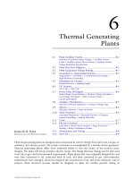
approximately 480 nT=min over the region (Fig. 16.1). A recent examination by Metatech of
historically large disturbance intensities indicated that disturbance levels greater than 2000 nT=min
have been observed even in contemporary storms on at least three occasions over the last 30 years at
geomagnetic latitudes of concern for the North American power grid infrastructure and most other
similar world locations: August 1972, July 1982, and March 1989. Anecdotal information from older
storms suggests that disturbance levels may have reached nearly 5000 nT=min, a level $10 times
greater than the environment which triggered the Hydro Quebec collapse (Kappenman, 2005). Both
observations and simulations indicate that as the intensity of the disturbance increases, the relative
levels of GICs and related power system impacts will also proportionately increase. Under these

scenarios, the scale and speed of problems that could occur on exposed power grids has the potential
to cause widespread and severe disruption of bulk power system operations. Therefore, as storm
environments reach higher intensity levels, it becomes more likely that these events will precipitate
widespread blackouts to exposed power grid infrastructures.
16.3 Weak Link in the Grid: Transformers
The primary concern with GIC is the effect that they have on the operation of a large power transformer.
Under normal conditions the large power transformer is a very efficient device for converting one
voltage level into another. Decades of design engineering and refinement have increased efficiencies and
capabilities of these complex apparatus to the extent that only a few amperes of AC exciting current are
necessary to provide the magnetic flux for the voltage transformation in even the largest modern power
transformer.
However, in the presence of GIC, the near-direct current essentially biases the magnetic circuit of the
transformer with resulting disruptions in performance. The three major effects produced by GIC in
transformers are (1) the increased reactive power consumption of the affected transformer, (2) the
ß 2006 by Taylor & Francis Group, LLC.
increased even and odd harmonics generated by the half-cycle saturation, and (3) the possibilities of
equipment damaging stray flux heating. These distortions can cascade problems by disrupting the
performance of other network apparatus, causing them to trip off-line just when they are most needed
to protect network integrity. For large storms, the spatial coverage of the disturbance is large and
hundreds of transformers can be simultaneously saturated, a situation that can rapidly escalate into a
network-wide voltage collapse. In addition, individual transformers may be damaged from overheating
due to this unusual mode of operation, which can result in long-term outages to key transformers in the
network. Damage of these assets can slow the full restoration of power grid operations.
Transformers use steel in their cores to enhance their transformation capability and efficiency, but this
core steel introduces nonlinearities into their performance. Common design practice minimizes the
effect of the nonlinearity while also minimizing the amount of core steel. Therefore, the transformers are
usually designed to operate over a predominantly linear range of the core steel characteristics (as shown
in Fig. 16.2) with only slightly nonlinear conditions occurring at the voltage peaks. This produces a
relatively small exciting current (Fig. 16.3). With GIC present, the normal operating point on the core
steel saturation curve is offset and the system voltage variation that is still impressed on the transformer

causes operation in an extremely nonlinear portion of the core steel characteristic for half of the AC cycle
(Fig. 16.2), hence, the term half-cycle saturation.
Because of the extreme saturation that occurs on half of the AC cycle, the transformer now draws an
extremely large asymmetrical exciting current. The waveform in Fig. 16.3 depicts a typical example
from field tests of the exciting current from a three-phase 600 MVA power transformer that has 75 A of
07:43 UT
07:45 UT07:44 UT
07:42 UT
FIGURE 16.1 Four minutes of a superstorm. Space weather conditions capable of threatening power system reliability
can rapidly evolve. The system operators at Hydro Quebec and other power system operators across North America faced
such conditions during the March 13, 1989 Superstorm. The above slides show the rapid development and movement of a
large geomagnetic field disturbance between the times 7:42 to 7:45 UT (2:42 to 2:45 EST) on March 13, 1989. The
disturbance of the magnetic field began intensifying over the eastern US–Canada border and then rapidly intensified
while moving to the west across North America over the span of a few minutes. With this rapid geomagnetic field
disturbance onset, the Hydro Quebec system went from normal operating conditions to complete collapse in a span of
just 90 s due to resulting GIC impacts on the grid. The magnetic field disturbances observed at the ground are caused by
large electrojet current variations that interact with the geomagnetic field. The dB=dt intensities ranged from 400 nT=min
at Ottawa at 7:44 UT to over 892 nT=min at Glen Lea. Large-scale rapid movement of this disturbance was evident.
ß 2006 by Taylor & Francis Group, LLC.
GIC in the neutral (25 A per phase). Spectrum analysis reveals this distorted exciting current to be rich
in even, as well as odd harmonics. As is well documented, the presence of even a small amount of GIC (3
to 4 A per phase or less) will cause half-cycle saturation in a large transformer.
Since the exciting current lags the system voltage by 908, it creates reactive power loss in the
transformer and the impacted power system. Under normal conditions, transformer reactive power
loss is very small. However, the several orders of magnitude increase in exciting current under half-cycle
saturation also results in extreme reactive power losses in the transformer. For example, the three-phase
reactive power loss associated with the abnormal exciting current of Fig. 16.3 produces a reactive power
loss of over 40 MVars for this transformer alone. The same transformer would draw less than 1 MVar
under normal conditions. Figure 16.4 provides a comparison of reactive power loss for two core types of
transformers as a function of the amount of GIC flow.

Under a geomagnetic storm condition in which a large number of transformers are experiencing a
simultaneous flow of GIC and undergoing half-cycle saturation, the cumulative increase in reactive
power demand can be significant enough to impact voltage regulation across the network, and in
extreme situations, lead to network voltage collapse.
The large and distorted exciting current drawn by the transformer under half-cycle saturation also
poses a hazard to operation of the network because of the rich source of even and odd harmonic currents
this injects into the network and the undesired interactions that these harmonics may cause with relay
and protective systems or other power system apparatus. Figure 16.5 summarizes the spectrum analysis
of the asymmetrical exciting current from Fig. 16.3. Even and odd harmonics are present typically in the
first 10 orders and the variation of harmonic current production varies somewhat with the level of GIC,
the degree of half-cycle saturation, and the type of transformer core.
With the magnetic circuit of the core steel saturated, the magnetic core will no longer contain the flow
of flux within the transformer. This stray flux will impinge upon or flow through adjacent paths such as
the transformer tank or core-clamping structures. The flux in these alternate paths can concentrate to
the densities found in the heating elements of a kitchen stove. This abnormal operating regime can
persist for extended periods as GIC flows from storm events can last for hours. The hot spots that may
then form can severely damage the paper-winding insulation, produce gassing and combustion of the
Effective GIC
Exciting current
(0,0)Ј
(0,0)
Voltage
FIGURE 16.2 The presence of GIC causes the transformer magnetization characteristics to be biased or offset due
to the DC. Therefore on one-half of the AC cycle, the transformer is driven into saturation by the combination
of applied voltage and DC bias. Normal excitation operation is shown in the left curve, the biased operation in
the right.
ß 2006 by Taylor & Francis Group, LLC.
transformer oil, or lead to other serious internal and or catastrophic failures of the transformer. Such
saturation and the unusual flux patterns which result, are not typically considered in the design process
and, therefore, a risk of damage or loss of life is introduced.

One of the more thoroughly investigated incidents of transformer stray flux heating occurred in the
Allegheny Power System on a 350 MVA 500=138 kV autotransformer at their Meadow Brook Substation
near Winchester, Virginia. The transformer was first removed from service on March 14, 1989, because
of high gas levels in the transformer oil which were a by-product of internal heating. The gas-in-oil
analysis showed large increases in the amounts of hydrogen, methane, and acetylene, indicating core and
tank heating. External inspection of the transformer indicated four areas of blistering or discolored paint
due to tank surface heating. In the case of the Meadow Brook transformer, calculations estimate the
flux densities were high enough in proximity to the tank to create hot spots approaching 4008C. Reviews
made by Allegheny Power indicated that similar heating events (though less severe) occurred in several
other large power transformers in their system due to the March 13 disturbance. Figure 16.6 is a
recording that Allegheny Power made on their Meadow Brook transformer during a storm in 1992. This
measurement shows an immediate transformer tank hot spot developing in response to a surge in GIC
5
−12
−6
0
6
12
18
24
240
246
252
258
264
270
276
282
288
294

300
10
Current (A)
15 20
Time (ms)
25 30 35 40
FIGURE 16.3 Under normal conditions, the excitation current of this 600 MVA 500=230 kV transformer is less
than 1% of transformer rated current. However, with 25 A=phase of GIC present, the excitation current drawn by the
transformer (top curve) is highly distorted by the half-cycle saturation conditions and has a large peak magnitude
rich in harmonics.
ß 2006 by Taylor & Francis Group, LLC.
entering the neutral of the transformer, while virtually no change is evident in the top oil readings.
Because the hot spot is confined to a relatively small area, standard bulk top oil or other over temperature
sensors would not be effective deterrents to use to alarm or limit exposures for the transformer to these
conditions.
Designing a large transformer that would be immune to GIC would be technically difficult and
prohibitively costly. The ampere turns of excitation (the product of the normal exciting current and the
0
25
50
75
100
3 Core
1 Ph
0
10
20
30
40
Reactive demand

(MVars)
GIC transformer neutral (A)
Transformer reactive demand
FIGURE 16.4 The exciting current drawn by half-cycle saturation conditions shown in Fig. 16.3 produces a
reactive power loss in the transformer as shown in the top plot. This reactive loss varies with GIC flow as shown.
This was measured from field tests of a three-phase bank of single-phase 500=230 kV transformers. Also shown in the
bottom curve is measured reactive demand vs. GIC from a 230=115 kV three-phase three-legged core-form
transformer. Transformer core design is a significant factor in estimating GIC reactive power impact.
0
10
20
30
40
50
Exciting current (A)
12345678910
Harmonic order
Transformer harmonics
FIGURE 16.5 The distorted transformer exciting current shown in Fig. 16.3 has even and odd harmonic current
distortion. This spectrum analysis was half-cycle saturation conditions resulting from a GIC flow of 25 A per phase.
ß 2006 by Taylor & Francis Group, LLC.
number of winding turns) generally determine the core steel volume requirements of a transformer.
Therefore, designing for unsaturated operation with the high level of GIC present would require a
core of excessive size. The ability to even assess existing transformer vulnerability is a difficult under-
taking and can only be confidently achieved in extensive case-by-case investigations. Each transformer
design (even from the same manufacturer) can contain numerous subtle design variations. These
variations complicate the calculation of how and at what density the stray flux can impinge on internal
structures in the transformer. However, the experience from contemporary space weather events is
revealing and potentially paints an ominous outcome for historically large storms that are yet to occur
on today’s infrastructure. As a case in point, during a September 2004 Electric Power Research Industry

workshop on transformer damage due to GIC, Eskom, the power utility that operates the power grid in
South Africa (geomagnetic latitudes À278 to À348), reported damage and loss of 15 large, high-voltage
transformers (400 kV operating voltage) due to the geomagnetic storms of late October 2003. This
damage occurred at peak disturbance levels of less than 100 nT=min in the region (Kappenman, 2005).
16.4 An Overview of Power System Reliability and Related
Space Weather Climatology
The maintenance of the functional integrity of the bulk electric systems (i.e., power systems reliability) at
all times is a very high priority for the planning and operation of power systems worldwide. Power
systems are too large and critical in their operation to easily perform physical tests of their reliability
performance for various contingencies. The ability of power systems to meet these requirements is
commonly measured by deterministic study methods to test the system’s ability to withstand probable
disturbances through computer simulations. Traditionally, the design criterion consists of multiple
outage and disturbance contingencies typical of what may be created from relatively localized terrestrial
weather impacts. These stress tests are then applied against the network model under critical load or
system transfer conditions to define important system design and operating constraints in the network.
GIC
0
50
100
150
200
External tank temp
Top oil
Temperature (°C)
Time
GIC and tank temperature
5/10/92
GIC (A)
−30
−20

−10
0
10
20
30
40
50
60
70
4:09
4:19
4:29
4:39
4:49
4:59
5:09
5:19
5:29
5:39
5:49
FIGURE 16.6 Transformer hot spot heating due to stray flux can be a concern in operation of a transformer with
GIC present. This transformer experienced stray flux heating that could be monitored with a thermocouple mounted
on the tank exterior surface. This storm demonstrated that the GIC and resulting half-cycle saturation produced a
rapid heating in the tank hot spot. Notice also that transformer top-oil temperature did not show any significant
change, indicating that the hot spot was relatively localized. (Courtesy Phil Gattens.)
ß 2006 by Taylor & Francis Group, LLC.
System impact studies for geomagnetic storm scenarios can now be readily performed on large
complex power systems. For cases in which utilities have performed such analysis, the impact
results indicate that a severe geomagnetic storm event may pose an equal or greater stress on the
network than most of the classic deterministic design criteria now in use. Further, by the very nature that

these storms impact simultaneously over large regions of the network, they arguably pose a greater
degree of threat for precipitating a system-wide collapse than more traditional threat scenarios.
The evaluation of power system vulnerability to geomagnetic storms is, of necessity, a two-stage
process. The first stage is one of assessing the exposure to the network posed by the climatology. In other
words, how large and how frequent can the storm driver be in a particular region? The second stage is
one of assessment of the stress that probable and extreme climatology events may pose to reliable
operation of the impacted network. This is measured through estimates of levels of GIC flow across
the network and the manifestation of impacts such as sudden and dramatic increases in reactive
power demands and implications on voltage regulation in the network. The essential aspects of risk
management become the weighing of probabilities of storm events against the potential consequential
impacts produced by a storm. From this analysis effort meaningful operational procedures can be
further identified and refined to better manage the risks resulting from storms of various intensities
(Kappenman et al., 2000).
Successive advances have been made in the ability to undertake detailed modeling of geomagnetic
storm impacts upon terrestrial infrastructures. The scale of the problem is enormous, the physical
processes entail vast volumes of the magnetosphere, ionosphere, and the interplanetary magnetic field
conditions that trigger and sustain storm conditions. In addition, it is recognized that important
aspects and uncertainties of the solid-earth geophysics need to be fully addressed in solving these
modeling problems. Further, the effects to ground-based systems are essentially contiguous to the
dynamics of the space environment. Therefore, the electromagnetic coupling and resulting impacts of
the environment on ground-based systems require models of the complex network topologies
overlaid on a complex geological base that can exhibit variation of conductivities that can span
five orders of magnitude.
These subtle variations in the ground conductivity play an important role in determining the
efficiency of coupling between disturbances of the local geomagnetic field caused by space environment
influences and the resulting impact to ground-based systems that can be vulnerable to GIC. Lacking full
understanding of this important coupling parameter hinders the ability to better classify the climatology
of space weather on ground-based infrastructures.
16.5 Geological Risk Factors and Geoelectric Field Response
Considerable prior work has been done to model the geomagnetic induction effects in ground-based

systems. As an extension to this fundamental work, numerical modeling of ground conductivity
conditions have been demonstrated to provide accurate replication of observed geoelectric field condi-
tions over a very broad frequency spectrum (Kappenman et al., 1997). Past experience has indicated
that 1D Earth conductivity models are sufficient to compute the local electric fields. Lateral hetero-
geneity of ground conductivity conditions can be significant over mesoscale distances (Kappenman,
2001). In these cases, multiple 1D models can be used in cases where the conductivity variations are
sufficiently large.
Ground conductivity models need to accurately reproduce geoelectric field variations that are caused
by the considerable frequency ranges of geomagnetic disturbance events from the large magnitude=low-
frequency electrojet-driven disturbances to the low amplitude but relatively high-frequency impulsive
disturbances commonly associated with magnetospheric shock events. This variation of electromagnetic
disturbances, therefore, require models accurate over a frequency range from 0.3 Hz to as low as
0.00001 Hz. At these low frequencies of the disturbance environments, diffusion aspects of ground
conductivities must be considered to appropriate depths. Therefore skin depth theory can be used in the
ß 2006 by Taylor & Francis Group, LLC.
frequency domain to determine the range of depths that are of importance. For constant Earth
conductivities, the depths required are more than several hundred kilometers, although the exact
depth is a function of the layers of conductivities present at a specific location of interest.
It is generally understood that the Earth’s mantle conductivity increases with depth. In most locations,
ground conductivity laterally varies substantially at the surface over mesoscale distances; these conduct-
ivity variations with depth can range from three to five orders of magnitude. Whereas surface
conductivity can exhibit considerable lateral heterogeneity, conductivity at depth is more uniform,
with conductivities ranging from 0.1 to 10 S=m at depths from 600 to 1000 km. If sufficient low-
frequency measurements are available to characterize ground conductivity profiles, models of ground
conductivity can be successfully applied over mesoscale distances and can be accurately represented by
the use of layered conductivity profiles or models.
For illustration of the importance of ground models on the response of geoelectric fields, a set of four
example ground models have been developed that illustrate the probable lower to upper quartile
response characteristics of most known ground conditions, considering there is a high degree of
uncertainty in the plausible diversity of upper layer conductivities. Figure 16.7 provides a plot of the

layered ground conductivity conditions for these four ground models to depths of 700 km. As shown,
there can be as much as four orders of magnitude variation in ground resistivity at various depths in the
upper layers. Models A and B have very thin surface layers of relatively low resistivity. Models A and C
are characterized by levels of relatively high resistivity until reaching depths exceeding 400 km, whereas
models B and D have high variability of resistivity in only the upper 50 to 200 km of depth.
800
700
600
500
400
Depth (km)
300
200
100
0
1 10 100 1,000
Resistivity (Ω m)
10,000 100,000
Ground A
Ground B
Ground C
Ground D
FIGURE 16.7 Resistivity profiles vs. depth for four example layered earth ground models.
ß 2006 by Taylor & Francis Group, LLC.
Figure 16.8 provides the frequency response characteristics for these same four-layered earth ground
models of Fig. 16.7. Each line plot represents the geoelectric field response for a corresponding incident
magnetic field disturbance at each frequency. Whereas each ground model has unique response
characteristics at each frequency, in general all ground models produce higher geoelectric field responses
as the frequency of the incident disturbance increases. Also shown on this plot are the relative differences
in geoelectric field response for the lowest and highest responding ground model at each decade of

frequency. This illustrates that the response between the lowest and highest responding ground model
can vary at discrete frequencies by more than a factor of 10. Also because the frequency content of an
impulsive disturbance event can have higher frequency content (for instance due to a shock), the
disturbance is acting upon the more responsive portion of the frequency range of the ground models
(Kappenman, 2004). Therefore, the same disturbance energy input at these higher frequencies produces
a proportionately larger response in geoelectric field. For example, in most of the ground models, the
geoelectric field response is a factor of 50 higher at 0.1 Hz compared to the response at 0.0001 Hz.
From the frequency response plots of the ground models as provided in Fig. 16.8, some of the
expected geoelectric field response due to geomagnetic field characteristics can be inferred. For example,
Ground C provides the highest geoelectric field response across the entire spectral range, therefore, it
would be expected that the time-domain response of the geoelectric field would be the highest for nearly
all B field disturbances. At low frequencies, Ground B has the lowest geoelectric field response whereas at
frequencies above 0.02 Hz, Ground A produces the lowest geoelectric field response. Because each of
these ground models has both frequency-dependent and nonlinear variations in response, the resulting
form of the geoelectric field waveforms would be expected to differ in form for the same B field input
disturbance. In all cases, each of the ground models produces higher relative increasing geoelectric field
response as the frequency of the incident B field disturbance increases. Therefore it should be expected
that a higher peak geoelectric field should result for a higher spectral content disturbance condition.
A large electrojet-driven disturbance is capable of producing an impulsive disturbance as shown
in Fig. 16.9, which reaches a peak delta B magnitude of $2000 nT with a rate of change (dB=dt)of
2400 nT=min. This disturbance scenario can be used to simulate the estimated geoelectric field response
of the four example ground models. Figure 16.10 provides the geoelectric field responses for each of the
1E-5 1E-4 1E-3 0.01 0.1
1E-5
1E-4
1E-3
0.01
0.1
Ground A
Ground B

Ground C
Ground D
Geoelectric field response of four ground models
V/km per nT
Frequency (Hz)
~Factor of 2
~Factor of 4
~Factor of 7
~Factor of 6
~Factor of 13
FIGURE 16.8 Frequency response of four example ground models of Fig. 16.1, max=min geoelectric field response
characteristics shown at various discrete frequencies.
ß 2006 by Taylor & Francis Group, LLC.
four ground models for this 2400 nT=min B field disturbance. As expected, the Ground C model
produces the largest geoelectric field reaching a peak of $15 V=km, whereas Ground A is next largest
and the Ground B model produces the smallest geoelectric field response. The Ground C geoelectric field
peak is more than six times larger than the peak geoelectric field for the Ground B model. It is also
00:00 15:00 30:00 45:00
0
500
1000
1500
2000
2500
B Field disturbance—2400 nT/min electrojet
B Intensity (nT)
Time (mm:ss)
FIGURE 16.9 Waveform of example electrojet-driven geomagnetic field disturbance with 2400 nT=min rate of
change intensity.
00:00 05:00 10:00 15:00 20:00

−2
0
2
4
6
8
10
12
14
16
18
Geoelectric field response—2400 nT/min electrojet
Ground A
Ground B
Ground C
Ground D
V/km
Time (mm:ss)
FIGURE 16.10 Geoelectric field response of the four example ground models to the 2400 nT=min disturbance
conditions of Fig. 16.3.
ß 2006 by Taylor & Francis Group, LLC.
evident that significant differences result in the overall shape and form of the geoelectric field response.
For example, the peak geoelectric field for the Ground A model occurs 17 s later than the time of
the peak geoelectric field for the Ground B model. In addition to the differences in the time of peak, the
waveforms also exhibit differences in decay rates. As is implied from this example, both the magnitudes
of the geoelectric field responses and the relative differences in responses between models will change
dependent on the source disturbance characteristics.
16.6 Power Grid Design and Network Topology Risk Factors
While the previous discussion on ground conductivity conditions are important in determining the
geoelectric field response, and in determining levels of GICs and their resulting impacts. Power grid

design is also an important factor in the vulnerability of these critical infrastructures, a factor in
particular that over time has greatly escalated the effective levels of GIC and operational impacts due
to these increased GIC flows. Unfortunately, most research into space weather impacts on technology
systems has focused upon the dynamics of the space environment. The role of the design and operation
of the technology system in introducing or enhancing vulnerabilities to space weather is often over-
looked. In the case of electric power grids, both the manner in which systems are operated and the
accumulated design decisions engineered into present-day networks around the world have tended to
significantly enhance geomagnetic storm impacts. The result is to increase the vulnerability of this
critical infrastructure to space weather disturbances.
Both growth of the power grid infrastructure and design of its key elements have acted to introduce
space weather vulnerabilities. The US high-voltage transmission grid and electric energy usage have
grown dramatically over the last 50 years in unison with increasing electricity demands of society.
The high-voltage transmission grid, which is the part of the power network that spans long distances,
couples almost like an antenna through multiple ground points to the geoelectric field produced by
disturbances in the geomagnetic field. From Solar Cycle 19 in the late 1950s through Solar Cycle 22 in
the early 1980s, the high-voltage transmission grid and annual energy usage have grown nearly tenfold
(Fig. 16.11). In short, the antenna that is sensitive to space weather disturbances is now very
large. Similar development rates of transmission infrastructure have occurred simultaneously in other
developed regions of the world.
As this network has grown in size, it has also grown in complexity and sets in place a compounding of
risks that are posed to the power grid infrastructures for GIC events. Some of the more important
changes in technology base that can increase impacts from GIC events include higher design voltages,
changes in transformer design, and other related apparatus. The operating levels of high-voltage
networks have increased from the 100–200 kV thresholds of the 1950s to 400 to 765 kV levels of
present-day networks. With this increase in operating voltages, the average per unit length circuit
resistance has decreased, whereas the average length of the grid circuit increases. In addition, power
grids are designed to be tightly interconnected networks, which present a complex circuit that is
continental in size. These interrelated design factors have acted to substantially increase the levels of
GIC that are possible in modern power networks.
In addition to circuit topology, GIC levels are determined by the size and the resistive impedance of

the power grid circuit itself when coupled with the level of geoelectric field, which result from the
geomagnetic disturbance event. Given a geoelectric field imposed over the extent of a power grid, a
current will be produced entering the neutral ground point at one location and exiting through other
ground points elsewhere in the network. This can be best illustrated by examining the typical range of
resistance per unit length for each kilovolt class of transmission lines and transformers.
As shown in Fig. 16.12, the average resistance per transmission line across the range of major
kilovolt-rating classes used in the current US power grid decreases by a factor of more than 10. Therefore
115 and 765 kV transmission lines of equal length can have a factor of $10 difference in total circuit
resistance. Ohm’s law indicates that the higher voltage circuits when coupled to the same geoelectric field
ß 2006 by Taylor & Francis Group, LLC.
0
500
1000
1500
2000
2500
3000
3500
4000
1950 1955 1960 1965 1970 1975 1980 1985 1990 1995 2000
Year
Electric energy usage (billion kWh)
0
20
40
60
80
100
120
140

160
180
High-voltage lines (miles ϫ 1000)
Annual electric energy usage
High-voltage transmission line miles
FIGURE 16.11 Growth of the US High Voltage Transmission Network and annual electric energy usage over the
past 50 years. In addition to increasing total network size, the network has grown in complexity with introduction of
higher kilovolt-rated lines that subsequently also tend to carry larger GIC flows. (Grid size derived from data in EHV
Transmission Line Reference Book and NERC Electricity Supply and Demand Database; energy usage statistics from
US Department of Energy—Energy Information Agency.)
0.001
0.01
0.1
1
kV Ratin
g
Resistance (Ω/km)
115 kV
138 kV
161 kV 230 kV
345 kV 500 kV
765 kV
FIGURE 16.12 Range of transmission line resistance for the major kilovolt-rating classes for transmission lines in
the US electric power grid infrastructure population. Also shown is a trend line of resistance weighted to average.
The lower R for the higher voltage lines will also cause proportionately larger GIC flows in this portion of the power
grid. (Derived from data in EHV Transmission Line Reference Book and from US Department of Energy, Energy
Information Agency and FERC Form 1 Database.)
ß 2006 by Taylor & Francis Group, LLC.
would result in as much as $10 times larger GIC flows in the higher voltage portions of the power grid.
The resistive impedance of large power system transformers follows a very similar pattern: the larger

the power capacity and kilovolt-rating, the lower the resistance of the transformer. In combination, these
design attributes will tend to collect and concentrate GIC flows in the higher kilovolt-rated equipment.
More important, the higher kilovolt-rated lines and transformers are key network elements, as they are
the long-distance heavy haulers of the power grid. The upset or loss of these key assets due to large GIC
flows can rapidly cascade into geographically widespread disturbances to the power grid.
Most power grids are highly complex networks with numerous circuits or paths and transformers for
GIC to flow through. This requires the application of highly sophisticated network and electromagnetic
coupling models to determine the magnitude and path of GIC throughout the complex power grid.
However for the purposes of illustrating the impact of power system design, a review will be provided
using a single-transmission line terminated at each end with a single transformer to ground connection.
To illustrate the differences that can occur in levels of GIC flow at higher voltage levels, the simple
demonstration circuit has also been developed at 138, 230, 345, 500, and 765 kV, which are common grid
voltages used in the United States and Canada. In Europe, voltages of 130, 275, and 400 kV are
commonly used for the bulk power grid infrastructures. For these calculations, a uniform 1.0 V=km
geoelectric field disturbance conditions are used, which means that the change in GIC levels will result
from changes in the power grid resistances alone. Also for uniform comparison purposes, a 100 km long
line is used in all kilovolt-rating cases.
Figure 16.13 illustrates the comparison of GIC flows that would result for various US infrastructure
power grid kilovolt ratings using the simple circuit and a uniform 1.0 V=km geoelectric field disturb-
ance. In complex networks, such as those in the United States, some scatter from this trend line is
possible due to normal variations in circuit parameters such as line resistances, etc., which can occur in
the overall population of infrastructure assets. Further, this was an analysis of simple ‘‘one-line’’
topology network, whereas real power grid networks have highly complex topologies, span large
geographic regions, and present numerous paths for GIC flow, all of which tend to increase total GIC
flows. Even this limited demonstration tends to illustrate that the power grid infrastructures of large
grids in the United States and other locations of the world are increasingly exposed to higher GIC flows
due to design changes that have resulted in reduced circuit resistance. Compounding this risk further,
the higher kilovolt portions of the network handle the largest bulk power flows and form the backbone
of the grid. Therefore the increased GIC risk is being placed at the most vital portions of this critical
GIC for 100 km line by kV rating

using average US grid resistances
0
20
40
60
80
100
120
138 230 345 500 765
kV Ratin
g
Neutral GIC (A)
FIGURE 16.13 Average neutral GIC flows vs. kilovolt rating for a 100 km demonstration transmission circuit.
ß 2006 by Taylor & Francis Group, LLC.
infrastructure. In the United States, 345, 500, and 765 kV transmission systems are widely spread
throughout and especially concentrated in areas of the United States with high population densities.
One of the best ways to illustrate the operational impacts of large GIC flows is to review the way in
which the GIC can distort the AC output of a large power transformer due to half-cycle saturation.
Under severe geomagnetic storm conditions, the levels of geoelectric field can be many times larger
than the uniform 1.0 V=km used in the prior calculations. Under these conditions even larger GIC flows
are possible. For example (see Fig. 16.14), the normal AC current waveform in the high-voltage winding
of a 500 kV transformer under normal load conditions is shown ($300 A rms, $400 A peak). With a
large GIC flow in the transformer, the transformer experiences extreme saturation of the magnetic core
for one-half of the AC cycle (half-cycle saturation). During this half-cycle of saturation, the magnetic
core of the transformer draws an extremely large and distorted AC current from the power grid. This
combines with the normal AC load current producing the highly distorted asymmetrically peaky
waveform that now flows in the transformer. As shown, AC current peaks that are present are nearly
twice as large compared to normal current for the transformer under this mode of operation. This
highly distorted waveform is rich in both even and odd harmonics, which are injected into the system
and can cause misoperations of sensors and protective relays throughout the network (Kappenman et al.,

1981, 1989).
The design of transformers also acts to further compound the impacts of GIC flows in the high-
voltage portion of the power grid. While proportionately larger GIC flows occur in these large
high-voltage transformers, the larger high-voltage transformers are driven into saturation at the same
few amperes of GIC exposure as those of lower voltage transformers. More ominously, another
compounding of risk occurs as these higher kilovolt-rated transformers produce proportionately higher
power system impacts than comparable lower voltage transformers. As shown in Fig. 16.15, because
reactive power loss in a transformer is a function of the operating voltage, the higher kilovolt-rated
transformers will also exhibit proportionately higher reactive power losses due to GIC. For example, a
765 kV transformer will have approximately six times larger reactive power losses for the same
magnitude of GIC flow as that of a 115 kV transformer.
500 kV Transformer AC current—normal and GIC-distorted
−800
−600
−400
−200
0
200
400
600
800
1000
Time (ms)
A
Normal
GIC-distorted
116.67100.0083.3366.6750.0033.33
16.67
0.00
FIGURE 16.14 500 kV Simple demonstration circuit simulation results: transformer AC currents and distortion

due to GIC.
ß 2006 by Taylor & Francis Group, LLC.
All transformers on the network can be exposed to similar conditions simultaneously due to the wide
geographic extent of most disturbances. This means that the network needs to supply an extremely large
amount of reactive power to each of these transformers or voltage collapse of the network could occur.
The combination of voltage regulation stress, which occurs simultaneously with the loss of key elements
due to relay misoperations can rapidly escalate to widespread progressive collapse of the exposed
interconnected network. An example of these threat conditions can be provided for the US power
grid for extreme but plausible geomagnetic storm conditions.
16.7 Extreme Geomagnetic Disturbance Events—
Observational Evidence
Both the space weather community and the power industry have not fully understood these design
implications. The application of detailed simulation models has provided tools for forensic analysis of
recent storm activity and when adequately validated can be readily applied to examine impacts due
to historically large storms. Some of the first reports of operational impacts to power systems date
back to the early 1940s and the level of impacts has progressively become more frequent and significant
as growth and development of technology has occurred in this infrastructure. In more contemporary
times, major power system impacts in the United States have occurred in storms in 1957, 1958, 1968,
1970, 1972, 1974, 1979, 1982, 1983, and 1989 and several times in 1991. Both empirical and model
extrapolations provide some perspective on the possible consequences of storms on present-day
infrastructures.
Historic records of geomagnetic disturbance conditions and, more important, geoelectric field mea-
surements provide a perspective on the ultimate driving force that can produce large GIC flows in power
grids. Because geoelectric fields and resulting GIC are caused by the rate of change of the geomagnetic
field, one of the most meaningful methods to measure the severity of impulsive geomagnetic field
0
10
20
30
40

50
60
70
0 102030405060708090100
Neutral GIC (A)
Reactive power (MVars)
115 kV
230 kV
345 kV
500 kV
765 kV
FIGURE 16.15 The impacts of GIC flows are further compounded by the behavior of transformers on the AC
transmission network. Larger GIC flows will tend to occur in the higher kilovolt-rated transformers. As shown above
these transformers also produce a proportionately larger reactive power consumption on the grid compared to the
same level of GIC flow in lower kilovolt-rated transformers. (From ‘‘Space Weather and the Vulnerability of Electric
Power Grids’’ J.G. Kappenman—NATO-ASI ESPRIT Conference, in press).
ß 2006 by Taylor & Francis Group, LLC.
disturbances is by the magnitude of the geomagnetic field change per minute, measured in nanoteslas
per minute. For example, the regional disturbance intensity that triggered the Hydro Quebec collapse
during the March 13, 1989 storm only reached an intensity of 479 nT=min. Large numbers of
power system impacts in the United States were also observed for intensities that ranged from 300 to
600 nT=min during this storm. However, the most severe rate of change in the geomagnetic field
observed during this storm reached a level of $2000 nT=min over the lower Baltic. The last such
disturbance with an intensity of $2000 nT=min over North America was observed during a storm on
August 4, 1972 when the power grid infrastructure was less than 40% of its current size.
Data assimilation models provide further perspectives on the intensity and geographic extent of the
intense dB=dt of the March 1989 Superstorm. Figure 16.16 provides a synoptic map of the ground level
geomagnetic field disturbance regions observed at time 22:00 UT. The previously mentioned lower Baltic
region observations are embedded in an enormous westward electrojet complex during this period of
time. Simultaneously with this intensification of the westward electrojet, an intensification of the

eastward electrojet occupies a region across midlatitude portions of the western US. The features of
the westward electrojet extend longitudinally $1208 and have a north–south cross-section ranging as
much as 58 to 108 in latitude.
Older storms provide even further guidance on the possible extremes of these specific electrojet-
driven disturbance processes. A remarkable set of observations was conducted on rail communication
circuits in Sweden that extend back nearly 80 years. These observations provide key evidence that
allow for estimation of the geomagnetic disturbance intensity of historically important storms in an era
where geomagnetic observatory data is unavailable. During a similarly intense westward electrojet
disturbance on July 13–14, 1982, a $100 km length communication circuit from Stockholm to
Torreboda measured a peak geopotential of 9.1 V=km (Lindahl). Simultaneous measurements at nearby
Lovo observatory in central Sweden measured a dB=dt intensity of $2600 nT=min at 24:00 UTon July 13.
FIGURE 16.16 Extensive westward electrojet-driven geomagnetic field disturbances at time 22:00 UT on
March 13, 1989.
ß 2006 by Taylor & Francis Group, LLC.
Figure 16.17 shows the delta Bx observed at BFE and Lovo during the peak disturbance times on July 13
and for comparison purposes the delta Bx observed at BFE during the large substorm on March 13,
1989. This illustrates that the comparative level of delta Bx is twice as large for the July 13, 1982 event
than that observed on March 13, 1989. The large delta Bx of >4000 nT for the July 1982 disturbance
suggests that these large field deviations are capable of producing even larger dB=dt impulses should
faster onset or collapse of the Bx field occur over the region (Kappenman, 2006).
As previously discussed, unprecedented power system impacts were observed in North America on
March 13–14, 1989 for storm intensities that reached levels of approximately 300–600 nT=min. However,
the investigation of very large storms indicates that storm intensities over many of these same US regions
could be as much as 4 to 10 times larger. These megastorms appear from historic data to be probable on
a 1-in-50 to 1-in-100 year time frame. Modern critical infrastructures have not as yet been exposed to
storms of this size. This increase in storm intensity causes a nearly proportional increase in resulting
stress to power grid operations. These storms also have a footprint that can simultaneously threaten
large geographic regions and can therefore plausibly trigger large regions of grid collapse.
16.8 Power Grid Simulations for Extreme Disturbance Events
Based upon these extreme disturbance events, a series of simulations were conducted for the entire US

power grid using electrojet-driven disturbance scenarios with the disturbance at 508 geomagnetic
latitude and at disturbance strengths of 2400, 3600, and 4800 nT=min. The electrojet disturbance
footprint was also positioned over North America with the previously discussed longitudinal dimensions
of a large westward electrojet disturbance. This extensive longitudinal structure will simultaneously
expose a large portion of the US power grid.
In this analysis of disturbance impacts, the level of cumulative increased reactive demands (MVars)
across the US power grid provides one of the more useful measures of overall stress on the network.
A comparison of geomagnetic disturbance conditions
Bx intensity—March 13–14, 1989 and July 13–14, 1982
−5000
−4000
−3000
−2000
−1000
0
1000
06070
80
Time (min)
nT
BFE—March 89
BFE—July 82
LOV—July 82
10 20 30 40 50 90 100 110 120
FIGURE 16.17 Comparison of observed delta Bx at Lovo and BFE during the July 13–14, 1982 and March 13, 1989
electrojet intensification events.
ß 2006 by Taylor & Francis Group, LLC.
This cumulative MVar stress was also determined for the March 13, 1989 storm for the US power grid,
which was estimated using the current system model as reaching levels of $7000 to 8000 MVars at times
21:44 to 21:57 UT. At these times, corresponding dB=dt levels in midlatitude portions of the United

States reached 350 to 545 nT=min as measured at various US observatories. This provides a comparison
benchmark that can be used to either compare absolute MVar levels or, the relative MVar level increases
for the more severe disturbance scenarios. The higher intensity disturbances of 2400 to 4800 nT=min will
have a proportionate effect on levels of GIC in the exposed network. GIC levels more than five times
larger than those observed during the above-mentioned periods in the March 1989 storm would be
probable. With the increase in GIC, a linear and proportionate increase in other power system impacts is
likely. For example, transformer MVar demands increase with increases in transformer GIC. As larger
GICs cause greater degrees of transformer saturation, the harmonic order and magnitude of distortion
currents increase in a more complex manner with higher GIC exposures. In addition, greater numbers of
transformers would experience sufficient GIC exposure to be driven into saturation, as generally higher
and more widely experienced GIC levels would occur throughout the extensive exposed power grid
infrastructure.
Figure 16.18 provides a comparison summary of the peak cumulative MVar demands that are
estimated for the US power grid for the March 1989 storm, and for the 2400, 3600, and 4800 nT=min
disturbances at the different geomagnetic latitudes. As shown, all of these disturbance scenarios are far
larger in magnitude than the levels experienced on the US power grid during the March 1989 Super-
storm. All reactive demands for the 2400 to 4800 nT=min disturbance scenarios would produce
unprecedented in size reactive demand increases for the US grid. The comparison with the MVar
demand from the March 1989 Superstorm further indicates that even the 2400 nT=min disturbance
scenarios would produce reactive demand levels at all of the latitudes that would be approximately six
times larger than those estimated in March 1989. At the 4800 nT=min disturbance levels, the reactive
demand is estimated, in total, to exceed 100,000 MVars. While these large reactive demand increases are
calculated for illustration purposes, impacts on voltage regulation and probable large-scale voltage
collapse across the network could conceivably occur at much lower levels.
This disturbance environment was further adapted to produce a footprint and onset progression that
would be more geospatially typical of an electrojet-driven disturbance, using both the March 13, 1989
and July 13, 1982 storms as a template for the electrojet pattern. For this scenario, the intensity of the
Comparison of US power grid reactive power demand increase
0
20,000

40,000
60,000
80,000
100,000
120,000
March 1989 estimates 2400 nT/min 3600 nT/min 4800 nT/min
Disturbance scenario
MVars
FIGURE 16.18 Comparison of estimated US power grid reactive demands during March 13, 1989 Superstorm and
2400, 3600, and 4800 nT=min disturbance scenarios at 508 geomagnetic latitude position over the United States.
ß 2006 by Taylor & Francis Group, LLC.
disturbance is decreased as it progresses from the eastern to western US. The eastern portions of the
United States are exposed to a 4800 nT=min disturbance intensity, while, west of the Mississippi, the
disturbance intensity decreases to only 2400 nT=min. The extensive reactive power increase and
extensive geographic boundaries of impact would be expected to trigger large-scale progressive collapse
conditions, similar to the mode in which the Hydro Quebec collapse occurred. The most probable
regions of expected power system collapse can be estimated based upon the GIC levels and reactive
demand increases in combination with the disturbance criteria as it applies to the US power pools.
Figure 16.19 provides a map of the peak GIC flows in the US power grid (size of circle at each node
indicates relative GIC intensity) and estimated boundaries of regions that likely could experience system
collapse due to this disturbance scenario. This example shows one of many possible scenarios for how a
large storm could unfold.
While these complex models have been rigorously tested and validated, this is an exceedingly complex
task with uncertainties that can easily be as much as a factor of two. However, just empirical evidence
alone suggests that power grids in North America that were challenged to collapse for storms of 400 to
600 nT=min over a decade ago, are not likely to survive the plausible but rare disturbances of 2000
to 5000 nT=min that long-term observational evidence indicates have occurred before and therefore may
be likely to occur again. Because large power system catastrophes due to space weather are not a zero
probability event and because of the large-scale consequences of a major power grid blackout, it is
important to discuss the potential societal and economic impacts of such an event should it ever reoccur.

The August 14, 2003 US Blackout event provides a good case study, the utilities and various municipal
organizations should be commended for the rapid and orderly restoration efforts that occurred.
However, it should also acknowledge that in many respects this blackout occurred during highly optimal
conditions, that were somewhat taken for granted and should not be counted upon in future blackouts.
For example, an outage on January 14 rather than August 14 could have meant coincident cold weather
conditions. Under these conditions, breakers and equipment at substations and power plants can be
more difficult to reenergize when they become cold. Geomagnetic storms as previously discussed can
also permanently damage key transformers on the grid which further burdens the restoration process,
and delays could rapidly cause serious public health and safety concerns.
Areas of probable power
system collapse
FIGURE 16.19 Regions of large GIC flows and possible power system collapse due to a 4800 nT=min disturbance
scenario.
ß 2006 by Taylor & Francis Group, LLC.
Because of the possible large geographic lay down of a severe storm event and resulting power grid
collapse, the ability to provide meaningful emergency aid and response to an impacted population
that may be in excess of 100 million people will be a difficult challenge. Even basic necessities such as
potable water and replenishment of foods may need to come from boundary regions that are unaffected
and these unaffected regions could be very remote to portions of the impacted US population centers.
As previously suggested adverse terrestrial weather conditions could cause further complications in
restoration and resupply logistics.
16.9 Conclusions
Contemporary models of large power grids and the electromagnetic coupling to these infrastructures by
the geomagnetic disturbance environment have matured to a level in which it is possible to achieve very
accurate benchmarking of storm geomagnetic observations and the resulting GIC. As abilities advance to
model the complex interactions of the space environment with the electric power grid infrastructures,
the ability to more rigorously quantify the impacts of storms on these critical systems also advances. This
quantification of impacts due to extreme space weather events is leading to the recognition that
geomagnetic storms are an important threat that has not been well recognized in the past.
References

Erinmez, I.A., Majithia, S., Rogers, C., Yasuhiro, T., Ogawa, S., Swahn, H., and Kappenman, J.G.,
Application of modelling techniques to assess geomagnetically induced current risks on the
NGC transmission system, CIGRE Paper 39-304, Session 2002.
Kappenman, J.G., Chapter 13: An introduction to power grid impacts and vulnerabilities from space
weather, in NATO-ASI Book on Space Storms and Space Weather Hazards, Vol. 38, edited by I.A.
Daglis, Kluwer Academic Publishers, NATO Science Series, 2001, pp. 335–361.
Kappenman, J.G., Chapter 14: Space weather and the vulnerability of electric power grids, in Effects of
Space Weather on Technology Infrastructure, Vol. 176, edited by I.A. Daglis, Kluwer Academic
Publishers, Norwell, 2004, pp. 257–286.
Kappenman, J.G., An overview of the impulsive geomagnetic field disturbances and power grid impacts
associated with the violent Sun–Earth connection events of 29–31 October 2003 and a compara-
tive evaluation with other contemporary storms, Space Weather, 3, S08C01, 2005, doi:10.1029=
2004SW000128.
Kappenman, J.G., Great geomagnetic storms and extreme impulsive geomagnetic field disturbance
events—an analysis of observational evidence including the great storm of May 1921, Advances
in Space Research, 38(2), 188–199, 2006.
Kappenman, J.G., Albertson, V.D., and Mohan, N., Current transformer and relay performance in the
presence of geomagnetically-induced currents, IEEE PAS Transactions, PAS-100, 1078–1088,
March 1981.
Kappenman, J.G., Carlson, D.L., and Sweezy, G.A., GIC effects on relay and CT performance,
Paper Presented at the EPRI Conference on Geomagnetically-Induced Currents, November 8–10,
San Francisco, CA, 1989.
Kappenman, J.G., Zanetti, L.J., and Radasky, W.A., Space weather from a user’s perspective: Geomag-
netic storm forecasts and the power industry, EOS Transactions of the American Geophysical Union,
78(4), 37–45, January 1997.
Kappenman, J.G., Radasky, W.A., Gilbert, J.L., and Erinmez, I.A., Advanced geomagnetic storm fore-
casting: A risk management tool for electric power operations, IEEE Plasma Society Special Issue on
Space Plasmas, 28(6), 2114–2121, December 2000.
ß 2006 by Taylor & Francis Group, LLC.