synchronous generators chuong (3)
Bạn đang xem bản rút gọn của tài liệu. Xem và tải ngay bản đầy đủ của tài liệu tại đây (713.42 KB, 55 trang )
© 2006 by Taylor & Francis Group, LLC
3-1
3
Prime Movers
3.1 Introduction 3-1
3.2 Steam Turbines
3-3
3.3 Steam Turbine Modeling
3-5
3.4 Speed Governors for Steam Turbines
3-10
3.5 Gas Turbines
3-11
3.6 Diesel Engines
3-12
Diesel-Engine Operation • Diesel-Engine Modeling
3.7 Stirling Engines 3-17
Summary of Thermodynamic Basic Cycles • The Stirling-Cycle
Engine • Free-Piston Stirling Engines Modeling
3.8 Hydraulic Turbines 3-24
Hydraulic Turbines Basics • A First-Order Ideal Model of
Hydraulic Turbines • Second- and Higher-Order Models of
Hydraulic Turbines • Hydraulic Turbine Governors • Reversible
Hydraulic Machines
3.9 Wind Turbines 3-39
Principles and Efficiency of Wind Turbines • The Steady-State
Model of Wind Turbines • Wind Turbine Models for Control
3.10 Summary 3-52
References
3-54
3.1 Introduction
Electric generators convert mechanical energy into electrical energy. The mechanical energy is produced
by prime movers. Prime movers are mechanical machines. They convert primary energy of a fuel or fluid
into mechanical energy. They are also called turbines or engines. The fossil fuels commonly used in prime
movers are coal, gas, oil, or nuclear fuel.
Essentially, the fossil fuel is burned in a combustor; thus, thermal energy is produced. Thermal energy
is then taken by a working fluid and turned into mechanical energy in the prime mover.
Steam is the working fluid for coal or nuclear fuel turbines. In gas turbines or in diesel or internal
combustion engines, the working fluid is the gas or oil in combination with air.
On the other hand, the potential energy of water from an upper-level reservoir may be turned into
kinetic energy that hits the runner of a hydraulic turbine, changes momentum and direction, and
produces mechanical work at the turbine shaft as it rotates against the “braking” torque of the electric
generator under electric load.
Wave energy is similarly converted into mechanical work in special tidal hydraulic turbines. Wind
kinetic energy is converted by wind turbines into mechanical energy.
A complete classification of prime movers is difficult due to the many variations in construction, from
topology to control. However, a simplified prime mover classification is described in Table 3.1.
© 2006 by Taylor & Francis Group, LLC
3-2 Synchronous Generators
In general, a prime mover or turbine drives an electric generator directly, or through a transmission
(at power less than a few megawatts [MW]), Figure 3.1, [1–3]. The prime mover is necessarily provided
with a so-called speed governor (in fact, a speed control and protection system) that properly regulates
the speed, according to electric generator frequency/power curves (Figure 3.2).
Notice that the turbine is provided with a servomotor that activates one or a few control valves that
regulate the fuel (or fluid) flow in the turbine, thus controlling the mechanical power at the turbine shaft.
The speed at the turbine shaft is measured precisely and compared with the reference speed. The speed
controller then acts on the servomotor to open or close control valves and control speed as required.
The reference speed is not constant. In alternating current (AC) power systems, with generators in parallel,
a speed drop of 2 to 3% is allowed, with power increased to the rated value [1–3].
The speed drop is required for two reasons:
• With a few generators of different powers in parallel, fair (proportional) power load sharing is provided.
• When power increases too much, the speed decreases accordingly, signaling that the turbine has
to be shut off.
In Figure 3.2, at point A at the intersection between generator power and turbine power, speed is
statically stable, as any departure from this point would provide the conditions (through motion equa-
tion) to return to it.
TABLE 3.1 Prime Mover Classification
Fuel
Working
Fluid Power Range Main Applications Type Observation
Coal or
nuclear fuel
Steam Up to 1500
MW/unit
Electric power systems Steam turbines High speed
Gas or oil Gas (oil)
+ air
From watts to
hundreds of
MW/unit
Large and distributed
power systems,
automotive applications
(vessels, trains, highway
and off-highway
vehicles), autonomous
power sources
Gas turbines, diesel
engines, internal
combustion
engines, Stirling
engines
With rotary but also
linear reciprocating
motion
Water energy Water Up to 1000
MW/unit
Large and distributed
electric power systems,
autonomous power
sources
Hydraulic turbines Medium and low
speeds, >75 rpm
Wind energy Air Up to 5 MW/unit Distributed power
systems, autonomous
power sources
Wind or wave
turbines
Speed down to
10 rpm
FIGURE 3.1 Basic prime-mover generator system.
Fuel
control
valve
Prime source
energy
Intermediate
energy
conversion/for
thermal turbines
Turbine
Servomotor
Speed governor
controller
Speed/power
reference curve
Frequency f1
power (Pe)
Electric
generator
Transmi-
ssion
Power grid
3~
Autonomous
load
Speed
sensor
© 2006 by Taylor & Francis Group, LLC
Prime Movers 3-3
With synchronous generators operating in a constant voltage and frequency power system, the speed
drop is very small, which implies strong strains on the speed governor due to inertia and so forth. It also
leads to slower power control. On the other hand, the use of doubly fed induction generators, or of AC
generators with full power electronics between them and the power system, would allow for speed
variation (and control) in larger ranges (±20% and more). That is, a smaller speed reference for lower
power. Power sharing between electric generators would then be done through power electronics in a
much faster and more controlled manner. Once these general aspects of prime mover requirements are
clarified, we will deal in some detail with prime movers in terms of principles, steady-state performance,
and models for transients. The main speed governors and their dynamic models are also included for
each main type of prime mover investigated here.
3.2 Steam Turbines
Coal, oil, and nuclear fuels are burned to produce high pressure, high temperature, and steam in a boiler.
The potential energy in the steam is then converted into mechanical energy in the so-called axial-flow
steam turbines.
The steam turbines contain stationary and rotating blades grouped into stages: high pressure (HP),
intermediate pressure (IP), low pressure (LP), and so forth. The high-pressure steam in the boiler is let
to enter — through the main emergency stop valves (MSVs) and the governor valves (GVs) — the
stationary blades, where it is accelerated as it expands to a lower pressure (Figure 3.3). Then the fluid is
guided into the rotating blades of the steam turbine, where it changes momentum and direction, thus
exerting a tangential force on the turbine rotor blades. Torque on the shaft and, thus, mechanical power,
are produced. The pressure along the turbine stages decreases, and thus, the volume increases. Conse-
quently, the length of the blades is lower in the high-pressure stages than in the lower-power stages.
The two, three, or more stages (HP, IP, and LP) are all, in general, on the same shaft, working in
tandem. Between stages, the steam is reheated, its enthalpy is increased, and the overall efficiency is
improved — up to 45% for modern coal-burn steam turbines.
Nonreheat steam turbines are built below 100 MW, while single-reheat and double-reheat steam
turbines are common above 100 MW, in general. The single-reheat tandem (same-shaft) steam turbine
is shown in Figure 3.3. There are three stages in Figure 3.3: HP, IP, and LP. After passing through the
MSVs and GVs, the high-pressure steam flows through the high-pressure stage where it experiences a
partial expansion. Subsequently, the steam is guided back to the boiler and reheated in the heat exchanger
to increase its enthalpy. From the reheater, the steam flows through the reheat emergency stop valve
FIGURE 3.2 The reference speed (frequency)/power curve.
1.0
A
0.5
Power (p.u.)
Generator power
Prime-mover power
1
Speed (p.u.)
0.95
0.9
0.8
© 2006 by Taylor & Francis Group, LLC
3-4 Synchronous Generators
(RSV) and intercept valve (IV) to the intermediate-pressure stage of the turbine, where again it expands
to do mechanical work. For final expansion, the steam is headed to the crossover pipes and through the
low pressure stage where more mechanical work is done. Typically, the power of the turbine is divided
as follows: 30% in the HP, 40% in the IP, and 30% in the LP stages. The governor controls both the GV
in the HP stage and the IV in the IP stage to provide fast and safe control.
During steam turbine starting — toward synchronous generator synchronization — the MSV is fully
open, while the GV and IV are controlled by the governor system to regulate the speed and power. The
governor system contains a hydraulic (oil) or an electrohydraulic servomotor to operate the GV and IV
and to control the fuel and air mix admission and its parameters in the boiler. The MSV and RSV are
used to quickly and safely stop the turbine under emergency conditions.
Turbines with one shaft are called tandem compound, while those with two shafts (eventually at
different speeds) are called cross-compound. In essence, the LP stage of the turbine is attributed to
a separate shaft (Figure 3.4). Controlling the speeds and powers of two shafts is difficult, though it
adds flexibility. Also, shafts are shorter. Tandem-compound (single-shaft) configurations are more
often used.
Nuclear units generally have tandem-compound (single-shaft) configurations and run at 1800 (1500)
rpm for 60 (50) Hz power systems. They contain one HP and three LP stages (Figure 3.5). The HP
exhaust passes through the moisture reheater (MSR) before entering the LP 1,2,3 stages in order to reduce
steam moisture losses and erosion. The HP exhaust is also reheated by the HP steam flow.
The governor acts upon the GV and the IV 1,2,3 to control the steam admission in the HP and LP
1,2,3 stages, while the MSV and the RSV 1,2,3 are used only for emergency tripping of the turbine. In
general, the GVs (control) are of the plug-diffuser type, while the IVs may be either the plug or the
butterfly type (Figure 3.6a and Figure 3.6b, respectively). The valve characteristics are partly nonlinear,
and, for better control, they are often “linearized” through the control system.
FIGURE 3.3 Single-reheat tandem-compound steam turbine.
Boiler
Reheater
MSV - Main emergency stop valve
GV - Governor valve
RSV - Reheat emergency stop valve
IV - Intercept valve
MSV
RSV
IV
GV
HP
IP
LP
Speed
sensor
Governor
Reference speed vs. power
To generator
shaft
Crossover
w
r
w
∗
r
(P
∗
)
© 2006 by Taylor & Francis Group, LLC
Prime Movers 3-5
3.3 Steam Turbine Modeling
The complete model of a multiple-stage steam turbine is rather involved. This is why we present here
first the simple steam vessel (boiler, reheated) model (Figure 3.7), [1–3], and derive the power expression
for the single-stage steam turbine.
The mass continuity equation in the vessel is written as follows:
(3.1)
where
V = the volume (m
3
)
Q = the steam mass flow rate (kg/sec)
ρ = the density of steam (kg/m
3
)
W = the weight of the steam in the vessel (kg).
Let us assume that the flow rate out of the vessel
Q
output
is proportional to the internal pressure in the
vessel:
FIGURE 3.4 Single-reheat cross-compound (3600/1800 rpm) steam turbine.
Boiler
Reheater
MSV
RSV
IV
GV
HP
IP
LP
Speed
sensor
Governor
Speed
sensor 2
Shaft to
generator 1,
3600 rpm
Shaft to
generator 2,
1800 rpm
w
∗
r1,2
(P
1,2
)
w
r1
w
r2
dW
dt
V
d
dt
input output
==−
ρ
© 2006 by Taylor & Francis Group, LLC
3-6 Synchronous Generators
(3.2)
where
P = the pressure (KPa)
P
0
and Q
0
= the rated pressure and flow rate out of the vessel
FIGURE 3.5 Typical nuclear steam turbine.
FIGURE 3.6 Steam valve characteristics: (a) plug-diffuser valve and (b) butterfly-type valve.
Q
Q
P
P
output
=
0
0
Boiler
MSV
GV
RSV1
MSR1 MSR2 MSR3
IV1
RSV2
IV2
RSV3
IV3
Governor
Speed
sensor
LP1 LP2 LP3
Shaft to
generator
w
r
HP
w
∗
r
(P
∗
)
1
1
0.5
0.5
Valve excursion
Valve flow rate
(b)
(a)
1
1
0.5
0.5
Valve excursion
Valve flow rate
© 2006 by Taylor & Francis Group, LLC
Prime Movers 3-7
As the temperature in the vessel may be considered constant,
(3.3)
Steam tables provide functions.
Finally, from Equation 3.1 through Equation 3.3, we obtain the following:
(3.4)
(3.5)
T
V
is the time constant of the steam vessel. With d/dt = s, the Laplace form of Equation 3.4 can be written
as follows:
(3.6)
The first-order model of the steam vessel has been obtained. The shaft torque
T
m
in modern steam
turbines is proportional to the flow rate:
(3.7)
So the power
P
m
is:
(3.8)
Example 3.1
The reheater steam volume of a steam turbine is characterized by Q
0
= 200 kg/sec, V = 100 m
3
, P
0
= 4000 kPa, and .
Calculate the time constant
T
R
of the reheater and its transfer function.
We use Equation 3.4 and Equation 3.5 and, respectively, Equation 3.6:
FIGURE 3.7 The steam vessel.
Q input
V
Q ouput
d
dt P
dP
dt
ρρ
=
∂
∂
⋅
(/)∂∂ρ P
QQ T
dQ
dt
input output V
output
−=
T
P
Q
V
P
V
=⋅
∂
∂
0
0
ρ
Q
QTs
output
input V
=
+⋅
1
1
TKQ
mm
=⋅
PT KQn
mmm m m
=⋅ = ⋅Ω 2π
∂∂=ρ/.P 0 004
© 2006 by Taylor & Francis Group, LLC
3-8 Synchronous Generators
Now consider the rather complete model of a single-reheat, tandem-compound steam turbine (Figure
3.3). We will follow the steam journey through the turbine, identifying a succession of time delays/time
constants.
The MSV and RSV are not shown in Figure 3.8, as they intervene only in emergency conditions.
The GVs modulate the steam flow through the turbine to provide for the required (reference) load
(power)/frequency (speed) control. The GV has a steam chest where substantial amounts of steam are
stored; and it is also found in the inlet piping. Consequently, the response of steam flow to a change in
a GV opening exhibits a time delay due to the charging time of the inlet piping and steam chest. This
time delay is characterized by a time constant
T
CH
in the order of 0.2 to 0.3 sec.
The IVs are used for rapid control of mechanical power (they handle 70% of power) during overspeed
conditions; thus, their delay time may be neglected in a first approximation.
The steam flow in the IP and LP stages may be changed with an increase in pressure in the reheater.
As the reheater holds a large amount of steam, its response-time delay is larger. An equivalent larger time
constant
T
RM
of 5 to 10 sec is characteristic of this delay [4].
The crossover piping also introduces a delay that may be characterized by another time constant
T
CO
.
We should also consider that the HP, IP, and LP stages produce
F
HP
, F
IP
, and F
LP
fractions of total
turbine power such that
F
HP
+ F
IP
+ F
LP
= 1 (3.9)
FIGURE 3.8 Single-reheat tandem-compound steam turbine.
From boiler
Steam chest
GV
(CV)
IV
Crossover piping
Shaft to generator
To condenser
HP IP LP
T
P
Q
V
P
R
=⋅
∂
∂
=××=
0
0
4000
200
100 0 004 8 0
ρ
sec
Q
Qs
output
input
=
+⋅
1
18
© 2006 by Taylor & Francis Group, LLC
Prime Movers 3-9
We may integrate these aspects of a steam turbine model into a structural diagram as shown in
Figure 3.9.
Typically, as already stated:
F
HP
= F
IP
= 0.3, F
LP
= 0.4, T
CH
≈ 0.2–0.3 sec, T
RH
= 5–9 sec, and T
CO
=
0.4–0.6 sec.
In a nuclear-fuel steam turbine, the IP stage is missing (
F
IP
= 0, F
LP
= 0.7), and T
RH
and T
CH
are notably
smaller. As
T
CH
is largest, reheat turbines tend to be slower than nonreheat turbines. After neglecting T
CO
and considering GV as linear, the simplified transfer function may be obtained:
(3.10)
The transfer function in Equation 3.10 clearly shows that the steam turbine has a straightforward
response to GV opening.
A typical response in torque (in per unit, P.U.) — or in power — to 1 sec ramp of 0.1 (P.U.) change
in GV opening is shown in Figure 3.10 for
T
CH
= 8 sec, F
HP
= 0.3, and T
CH
= T
CO
= 0.
In enhanced steam turbine models involving various details, such as IV, more rigorous representation
counting for the (fast) pressure difference across the valve may be required to better model various
intricate transient phenomena.
FIGURE 3.9 Structural diagram of single-reheat tandem-compound steam turbine.
FIGURE 3.10 Steam turbine response to 0.1 (P.U.) 1 sec ramp change of GV opening.
GV
Main
steam
pressure
Inlet and
steam chest delay
HP
flow
HP
pressure
Reheater delay
Intercept
valve
IV
position
IP
flow
Crossover
delay
Tm
turbine
torque
+
+
+
+
−
F
HP
F
IP
F
LP
Valve
position
1
1 + sT
CH
1
1 + sT
RH
1
1 + sT
CO
1
ΔT
m
(P.U.) ΔV
GV
(P.U.)
0.9
1
234
Time (s)
Valve
opening (P.U.)
Torque (P.U.) or power (P.U.)
5
Δ
Δ
Tm
V
sF T
sT sT
GV
HP RH
CH RH
≈
+
()
+
()
+
()
1
11
© 2006 by Taylor & Francis Group, LLC
3-10 Synchronous Generators
3.4 Speed Governors for Steam Turbines
The governor system of a turbine performs a multitude of functions, including the following [1–4]:
• Speed (frequency)/load (power) control: mainly through GVs
• Overspeed control: mainly through the IV
• Overspeed trip: through MSV and RSV
• Start-up and shutdown control
The speed/load (frequency/power) control (Figure 3.2) is achieved through the control of the GV to
provide linearly decreasing speed with load, with a small speed drop of 3 to 5%. This function allows for
paralleling generators with adequate load sharing. Following a reduction in electrical load, the governor
system has to limit overspeed to a maximum of 120%, in order to preserve turbine integrity. Reheat-type
steam turbines have two separate valve groups (GV and IV) to rapidly control the steam flow to the turbine.
The objective of the overspeed control is set to about 110 to 115% of rated speed to prevent overspeed
tripping of the turbine in case a load rejection condition occurs.
The emergency tripping (through MSV and RSV — Figure 3.3 and Figure 3.5) is a protection solution
in case normal and overspeed controls fail to limit the speed to below 120%.
A steam turbine is provided with four or more GVs that admit steam through nozzle sections distrib-
uted around the periphery of the HP stage. In normal operation, the GVs are open sequentially to provide
better efficiency at partial load. During the start-up, all the GVs are fully open, and stop valves control
steam admission.
Governor systems for steam turbines evolve continuously. Their evolution mainly occurred from
mechanical-hydraulic systems to electrohydraulic systems [4].
In some embodiments, the main governor systems activate and control the GV, while an auxiliary
governor system operates and controls the IV [4]. A mechanical-hydraulic governor generally contains
a centrifugal speed governor (controller), that has an effect that is amplified through a speed relay to
open the steam valves. The speed relay contains a pilot valve (activated by the speed governor) and a
spring-loaded servomotor (Figure 3.11a and Figure 3.11b).
In electrohydraulic turbine governor systems, the speed governor and speed relay are replaced by
electronic controls and an electric servomotor that finally activates the steam valve.
In large turbines an additional level of energy amplification is needed. Hydraulic servomotors are used
for the scope (Figure 3.12). By combining the two stages — the speed relay and the hydraulic servomotor
— the basic turbine governor is obtained (Figure 3.13).
FIGURE 3.11 Speed relay: (a) configuration and (b) transfer function.
Oil
supply
Oil drain
Steam valve
Mechanical
spring
Servomotor
Mechanical
speed governor
Pilot valve
T
SR
= 0.1–0.3s
K
SR
1 + sT
SR
(a)
(b)
© 2006 by Taylor & Francis Group, LLC
Prime Movers 3-11
For a speed drop of 4% at rated power, K
SR
= 25 (Figure 3.12). A similar structure may be used to
control the IV [2].
Electrohydraulic governor systems perform similar functions, but by using electronics control in the
lower power stages, they bring more flexibility, and a faster and more robust response. They are provided
with acceleration detection and load power unbalance relay compensation. The structure of a generic
electrohydraulic governor system is shown in Figure 3.14. Notice the two stages in actuation: the elec-
trohydraulic converter plus the servomotor, and the electronic speed controller.
The development of modern nonlinear control (adaptive, sliding mode, fuzzy, neural networks, H
∞
,
etc.) [5] led to the recent availability of a wide variety of electronic speed controllers or total steam
turbine-generator controllers [6]. These, however, fall beyond the scope of our discussion here.
3.5 Gas Turbines
Gas turbines burn gas, and that thermal energy is then converted into mechanical work. Air is used as
the working fluid. There are many variations in gas turbine topology and operation [1], but the most
used one seems to be the open regenerative cycle type (Figure 3.15).
The gas turbine in Figure 3.14 consists of an air compressor (C) driven by the turbine (T) and the
combustion chamber (CH). The fuel enters the combustion chamber through the GV, where it is mixed
with the hot-compressed air from the compressor. The combustion product is then directed into the
turbine, where it expands and transfers energy to the moving blades of the gas turbine. The exhaust gas
heats the air from the compressor in the heat exchanger. The typical efficiency of a gas turbine is 35%.
FIGURE 3.12 Hydraulic servomotor structural diagram.
FIGURE 3.13 Basic turbine governor.
FIGURE 3.14 Generic electrohydraulic governing system.
1
T
SM
1
S
Speed
relay
output
L
s2
L
s1
1.0
Valve stroke
Position limiter
0
−
Rate
limiter
Δω
1
K
SR
Load
reference
Speed
relay
L
S2
L
S1
1.0
0
−
Position limiter
GV
flow
1
1 + sT
SR
1
T
SM
1
s
Speed reference
Electronic speed
controller
Electrohydraulic
converter
Pilot
valve
Feedback
Servomotor
GV
flow
Valve position
Load
reference
Steam
pressure
Steam
flow
feedback
−
−
w
r
w
∗
r
© 2006 by Taylor & Francis Group, LLC
3-12 Synchronous Generators
More complicated cycles, such as compressor intercooling and reheating or intercooling with regeneration
and recooling, are used for further (slight) improvements in performance [1].
The combined- and steam-cycle gas turbines were recently proven to deliver an efficiency of 55% or
even slightly more. The generic combined-cycle gas turbine is shown in Figure 3.16.
The exhaust heat from the gas turbine is directed through the heat recovery boiler (HRB) to produce
steam, which, in turn, is used to produce more mechanical power through a steam turbine section on
the same shaft. With the gas exhaust exiting the gas turbine above 500°C and supplementary fuel burning,
the HRB temperature may rise further than the temperature of the HP steam, thus increasing efficiency.
Additionally, some steam for home (office) heating or process industries may be delivered.
Already in the tens of MW, combined-cycle gas turbines are becoming popular for cogeneration in
distributed power systems in the MW or even tenths and hundreds of kilowatts per unit. Besides efficiency,
the short construction time, low capital cost, low SO
2
emission, little staffing necessary, and easy fuel
(gas) handling are all main merits of combined-cycle gas turbines. Their construction at very high speeds
(tens of krpm) up to the 10 MW range, with full-power electronics between the generator and the
distributed power grid, or in stand-alone operation mode at 50(60) Hz, make the gas turbines a way of
the future in this power range.
3.6 Diesel Engines
Distributed electric power systems, with distribution feeders at approximately 12 kV, standby power sets
ready for quick intervention in case of emergency or on vessels, locomotives, or series or parallel hybrid
vehicles, and power-leveling systems in tandem with wind generators, all make use of diesel (or internal
combustion) engines as prime movers for their electric generators. The power per unit varies from a few
tenths of a kilowatt to a few megawatts.
As for steam or gas turbines, the speed of a diesel-engine generator set is controlled through a speed
governor. The dynamics and control of fuel–air mix admission are very important to the quality of the
electric power delivered to the local power grid or to the connected loads, in stand-alone applications.
3.6.1 Diesel-Engine Operation
In four-cycle internal combustion engines [7], and the diesel engine is one of them, with the period of
one shaft revolution T
REV
= 1/n (n is the shaft speed in rev/sec), the period of one engine power stroke T
PS
is
FIGURE 3.15 Open regenerative cycle gas turbine.
Exhaust
Heat exchanger
Air inlet
Combustion
chamber
(CH)
Fuel input
(governor valve)
Compressor
(C)
Gas
turbine
(T)
Shaft to
generator
© 2006 by Taylor & Francis Group, LLC
Prime Movers 3-13
(3.11)
The frequency of power stroke f
PS
is as follows:
(3.12)
For an engine with N
c
cylinders, the number of cylinders that fire each revolution, N
f
, is
(3.13)
The cylinders are arranged symmetrically on the crankshaft, so that the firing of the N
f
cylinders is
uniformely spaced in angle terms. Consequently, the angular separation (θ
c
) between successive firings
in a four-cycle engine is as follows:
(3.14)
The firing angles for a twelve-cylinder diesel engine are illustrated in Figure 3.17a, while the two-
revolution sequence is intake (I), compression (C), power (P), and exhaust (E) (Figure 3.17b). The twelve-
FIGURE 3.16 Combined-cycle unishaft gas turbine.
Air inlet
C
CH
GV1
GV2
Gas
turbine
(T)
Steam
turbine
(T)
Fuel in
Heat recovery
boiler
Exhaust
HRB
TT
PS REV
= 2
f
T
PS
PS
=
1
N
N
f
c
=
2
θ
c
c
N
=
720
0
© 2006 by Taylor & Francis Group, LLC
3-14 Synchronous Generators
cylinder timing is shown in Figure 3.18. There are three cylinders out of twelve firing simultaneously at
steady state. The resultant shaft torque of one cylinder varies with shaft angle, as shown in Figure 3.19.
The compression torque is negative, while during the power cycle, it is positive. With twelve cylinders,
the torque will have much smaller pulsations, with twelve peaks over 720° (period of power engine stroke)
— see Figure 3.20. Any misfire in one or a few of the cylinders would produce severe pulsations in the
torque that would reflect as a flicker in the generator output voltage [8].
Large diesel engines generally have a turbocharger (Figure 3.21) that notably influences the dynamic
response to perturbations by its dynamics and inertia [9]. The turbocharger is essentially an air com-
pressor that is driven by a turbine that runs on the engine exhaust gas. The compressor provides
compressed air to the engine cylinders. The turbocharger works as an energy recovery device with about
2% power recovery.
3.6.2 Diesel-Engine Modeling
A diagram of the general structure of a diesel engine with turbocharger and control is presented in
Figure 3.22.
The following are the most important components:
• The actuator (governor) driver that appears as a simple gain K
3
.
FIGURE 3.17 Twelve-cylinder four-cycle diesel engine: (a) configuration and (b) sequence.
FIGURE 3.18 Twelve-cylinder engine timing.
1
7
2
3
9
4
5
6
10
8
(a)
(b)
720°
1st revolution
ICPE
2nd revolution
1
2
3
4
5
6
7
8
9
10
11
12
abc
© 2006 by Taylor & Francis Group, LLC
Prime Movers 3-15
• The actuator (governor) fuel controller that converts the actuator’s driver into an equivalent fuel
flow, Φ. This actuator is represented by a gain K
2
and a time constant (delay) τ
2
, which is dependent
on oil temperature, and an aging-produced backlash.
• The inertias of engine J
E
, turbocharger J
T
, and electric generator (alternator) J
G
.
• The flexible coupling that mechanically connects the diesel engine to the alternator (it might also
contain a transmission).
• The diesel engine is represented by the steady-state gain K
1
— constant for low fuel flow Φ and
saturated for large Φ, multiplied by the equivalence ratio factor (erf) and by a time constant τ
1
.
• The erf depends on the engine equivalence ratio (eer), which, in turn, is the ratio of fuel/air
normalized by its stoichiometric value. A typical variation of erf with eer is shown in Figure 3.22.
In essence, erf is reduced, because when the ratio of fuel/air increases, incomplete combustion
occurs, leading to low torque and smoky exhaust.
• The dead time of the diesel engine is composed of three delays: the time elapsed until the actuator
output actually injects fuel into the cylinder, fuel burning time to produce torque, and time until
all cylinders produce torque at the engine shaft:
FIGURE 3.19 P.U. torque/angle for one cylinder.
FIGURE 3.20 P.U. torque vs. shaft angle in a 12-cylinder ICE (internal combustion engine).
1
0.75
0.5
0.25
0
−0.25
−100°−50° 50°
0
Negative
(compression)
torque
Positive
(power)
torque
100°
1.1
1.0
0.9
P.U. torque
0.8
0.4
120° 240° 360° 480° 560° 720°
Shaft angle
© 2006 by Taylor & Francis Group, LLC
3-16 Synchronous Generators
FIGURE 3.21 Diesel engine with turbocharger.
FIGURE 3.22 Diesel engine with turbocharger and controller.
Compressor
Turbine
Exhaust
Airbox
Intercooler
Engine
Gear
train
To generator
Clutch
Droop
Backlash
Actuator
(governor)
Turbine
Compressor torque
erf
n
E
n
G
T
E
Equivalence ratio compensation
Net
torque
Load
disturbance
Coupling
(flexible)
erf
eer
1
0.7
0.5 1.2
T
T
T
C
n
T
Φ
i
K
3
Control
Identification
Ref.
speed
K
2
1 + st
2
1
sJ
T
1
sJ
E
1
sJ
G
K
1
e
− st
1
−
−
−
−
−
© 2006 by Taylor & Francis Group, LLC
Prime Movers 3-17
(3.15)
where n
E
is the engine speed.
The turbocharger acts upon the engine in the following ways:
• It draws energy from the exhaust to run its turbine; the more fuel in the engine, the more exhaust
is available.
• It compresses air at a rate that is a nonlinear function of speed; the compressor is driven by the
turbine, and thus, the turbine speed and ultimate erf in the engine are influenced by the airflow rate.
• The turbocharger runs freely at high speed, but it is coupled through a clutch to the engine at low
speeds, to be able to supply enough air at all speeds; thus, the system inertia changes at low speeds,
by including the turbocharger inertia.
Any load change leads to transients in the system pictured in Figure 3.22 that may lead to oscillations
due to the nonlinear effects of fuel–air flow — equivalence ratio factor — inertia. As a result, there will
be either too little or too much air in the fuel mix. In the first case, smoky exhaust will be apparent. In
the second situation, not enough torque will be available for the electric load, and the generator may
pull out of synchronism. This situation indicates that proportional integral (PI) controllers of engine
speed are not adequate, and nonlinear controllers (adaptive, variable structure, etc.) are required [10].
A higher-order model may be adopted both for the actuator [11, 12] and for the engine [13] to better
simulate in detail the diesel-engine performance for transients and control.
3.7 Stirling Engines
Stirling engines are part of the family of thermal engines: steam turbines, gas turbines, spark-ignited
engines, and diesel engines. They were already described briefly in this chapter, but it is time now to
dwell a little on the thermodynamic engine cycles to pave the way for our discussion on Stirling engines.
3.7.1 Summary of Thermodynamic Basic Cycles
The steam engine, invented by James Watt, is a continuous combustion machine. Subsequently, the steam
is directed from the boiler to the cylinders (Figure 3.23a and Figure 3.23b). The typical four steps of the
steam engine (Figure 3.23a) are as follows:
• Isochoric compression (1–1′) followed by isothermal expansion (1′–2): The hot steam enters the
cylinder through the open valve at constant volume; it then expands at constant temperature.
• Isotropic expansion: Once the valve is closed, the expansion goes on until the maximum volume
is reached (3).
• Isochoric heat regeneration (3–3) and isothermal compression (3′–4): The pressure drops at
constant volume, and then the steam is compressed at constant temperature.
• Isentropic compression takes place after the valve is closed and the gas is mechanically compressed.
An approximate formula for thermal efficiency η
th
is as follows [13]:
(3.16)
where
ε = V
3
/V
1
is the compression ratio
ρ = V
2
/V
1
= V
3
/V
4
is the partial compression ratio
x = p
1
′/p
1
is the pressure ratio
τ
1
2
≈+ +A
B
n
C
n
E
E
η
ρρ
ερ
th
K
K
K
xK
=−
−+
−+ −
−
−
1
11
11
1
1
()(ln)
()( )ln
© 2006 by Taylor & Francis Group, LLC
3-18 Synchronous Generators
For ρ = 2, x = 10, K = 1.4, and ε = 3, η
th
= 31%.
The gas turbine engine fuel is also continuously combusted in combination with precompressed air.
The gas expansion turns the turbine shaft to produce mechanical power. The gas turbines work on a
Brayton cycle (Figure 3.24a and Figure 3.24b). The four steps of a Brayton cycle are as follows:
• Isentropic compression
• Isobaric input of thermal energy
• Isentropic expansion (work generation)
• Isobaric thermal energy loss
Similarly, with T
1
/T
4
= T
2
/T
3
for the isentropic steps, and the injection ratio ρ = T
3
/T
2
, the thermal
efficiency η
th
is as follows:
FIGURE 3.23 The steam engine “cycle”: (a) the four steps and (b) PV diagram.
FIGURE 3.24 Brayton cycle for gas turbines: (a) PV diagram and (b) TS diagram.
D
1
Dʹ
D
2
Dʹ
D
3
Dʹ
D
4
Dʹ
(a)
P
1'
1
2
4
3'
3
V
3
V
1
Volume
(b)
P
23
Isentropic
processes
14
V
(a)
Te mp
2
3
1
4
S (entropy)
(b)
© 2006 by Taylor & Francis Group, LLC
Prime Movers 3-19
(3.17a)
With ideal, complete, heat recirculation:
(3.17b)
Gas turbines are more compact than other thermal machines; they are easy to start and have low
vibration, but they also have low efficiency at low loads (ρ small) and tend to have poor behavior during
transients.
The spark-ignition (Otto) engines work on the cycle shown in Figure 3.25a and Figure 3.25b. The
four steps are as follows:
• Isentropic compression
• Isochoric input of thermal energy
• Isentropic expansion (kinetic energy output)
• Isochoric heat loss
The ideal thermal efficiency η
th
is
(3.18)
where
(3.19)
for isentropic processes. With a high compression ratio (say ε = 9) and the adiabatic coefficient K = 1.5,
η
th
= 0.66.
FIGURE 3.25 Spark-ignition engines: (a) PV diagram and (b) TS diagram.
η
ρ
th
T
T
≈−1
1
4
2
η
ρ
th
≈−1
1
η
ε
ε
th
K
VV=− =
−
1
1
1
12
;/
T
T
T
T
V
V
K
K
4
3
1
2
3
4
1
1
1
==
⎛
⎝
⎜
⎞
⎠
⎟
=
−
−
ε
P
2
3
1
4
V
(a)
(b)
T
2
3
1
4
S
© 2006 by Taylor & Francis Group, LLC
3-20 Synchronous Generators
The diesel-engine cycle is shown in Figure 3.26. During the downward movement of the piston, an
isobaric state change takes place by controlled injection of fuel:
(3.20)
Efficiency decreases when load ρ increases, in contrast to spark-ignition engines for the same ε. Lower
compression ratios (ε) than those for spark-ignition engines are characteristic of diesel engines so as to
obtain higher thermal efficiency.
3.7.2 The Stirling-Cycle Engine
The Stirling engine (developed in 1816) is a piston engine with continuous heat supply (Figure 3.27a
through Figure 3.27c). In some respects, the Stirling cycle is similar to the Carnot cycle (with its two
isothermal steps). It contains two opposed pistons and a regenerator in between. The regenerator is
made in the form of strips of metal. One of the two volumes is the expansion space kept at a high
temperature T
max
, while the other volume is the compression space kept at a low temperature T
min
.
Thermal axial conduction is considered negligible. Suppose that the working fluid (all of it) is in the
cold compression space.
During compression (steps 1 to 2), the temperature is kept constant because heat is extracted from
the compression space cylinder to the surroundings.
During the transfer step (steps 2 to 3), both pistons move simultaneously; the compression piston
moves toward the regenerator, while the expansion piston moves away from it. So, the volume stays
constant. The working fluid is, consequently, transferred through the porous regenerator from compres-
sion to expansion space and is heated from T
min
to T
max
. An increase in pressure also takes place between
steps 2 and 3. In the expansion step (3 to 4), the expansion piston still moves away from the regenerator,
but the compression piston stays idle at an inner dead point. The pressure decreases, and the volume
FIGURE 3.26 The diesel-engine cycle.
P
23
1
4
V
3
V
V
1
V
2
ρ
η
ε
ρ
ρ
==
=− ⋅
−
−
−
V
V
T
T
K
th
K
K
3
2
3
2
1
1
11 1
1
;
© 2006 by Taylor & Francis Group, LLC
Prime Movers 3-21
increases, but the temperature stays constant, because heat is added from an external source. Then, again,
a transfer step (step 4 to step 1) occurs, with both pistons moving simultaneously to transfer the working
fluid (at constant volume) through the regenerator from the expansion to the compression space. Heat
is transferred from the working fluid to the regenerator, which cools at T
min
in the compression space.
The ideal thermal efficiency η
th
is as follows:
(3.21)
So, it is heavily dependent on the maximum and minimum temperatures, as is the Carnot cycle.
Practical Stirling-type cycles depart from the ideal. The practical efficiency of Stirling-cycle engines is
much lower: η
th
< η
th
K
th
(K
th
< 0.5, in general).
Stirling engines may use any heat source and can use various working fuels, such as air, hydrogen, or
helium (with hydrogen the best and air the worst). Typical total efficiencies vs. high pressure/liter density
FIGURE 3.27 The Stirling engine: (a) mechanical representation and (b) and (c) the thermal cycle.
Hot volume (expansion) Cold volume (compression)
Piston
Heater
Regenerator
Cooler
Piston
p
K
, T
E
p
K
, T
K
1
V
P
To cooler
2
3
Close cycle
(by regenerator)
4
From heater
1
S
T
T
min
T
max
2
3
4
(a)
(b)
(c)
η
th
i
T
T
=−1
min
max
© 2006 by Taylor & Francis Group, LLC
3-22 Synchronous Generators
are shown in Figure 3.28 [14] for three working fluids at various speeds. As the power and speed go up,
the power density decreases. Methane may be a good replacement for air for better performance.
Typical power/speed curves of Stirling engines with pressure p are shown in Figure 3.29a. And, the
power/speed curves of a potential electric generator, with speed, and voltage V as a parameter, appear in
Figure 3.29b. The intersection at point A of the Stirling engine and the electric generator power/speed
curves looks clearly like a stable steady-state operation point. There are many variants for rotary-motion
Stirling engines [14].
3.7.3 Free-Piston Stirling Engines Modeling
Free-piston linear-motion Stirling engines were recently developed (by Sunpower and STC companies)
for linear generators for spacecraft or home electricity production (Figure 3.30) [15].
FIGURE 3.28 Efficiency/power density of Stirling engines.
FIGURE 3.29 Power/speed curves: (a) the Stirling engine and (b) the electric generator.
60
125
250
500
500
750
750
1000
1500
H
2
225 HP/cylinder
T
max
= 700°C
T
min
= 25°C
Gas pressure: 1100 N/cm
2
1000
He
400 rpm
Air
20 40 60
Power density (HP/liter)
50
η (%) total
40
30
20
10
Methane
P (pressure)
P
Speed
(a)
(b)
V (voltage)
A
P
el
Speed
© 2006 by Taylor & Francis Group, LLC
Prime Movers 3-23
The dynamic equations of the Stirling engine (Figure 3.30) are as follows:
(3.22)
for the normal displacer, and
(3.23)
for the piston, where
A
d
= the displacer rod area (m
2
)
D
d
= the displacer damping constant (N/msec)
P
d
= the gas spring pressure (N/m
2
)
P = the working gas pressure (N/m
2
)
D
p
= the piston damping constant (N/msec)
X
d
= the displacer position (m)
X
p
= the power piston position (m)
A = the cylinder area (m
2
)
M
d
= the displacer mass (kg)
M
p
= the power piston mass (kg)
F
elm
= the electromagnetic force (of linear electric generator) (N)
Equation 3.22 through Equation 3.23 may be linearized as follows:
(3.24)
FIGURE 3.30 Linear Stirling engine with free-piston displacer mover.
Heater
Regenerator
Cooler
Alternator
Piston
Cold space
Gas spring
(pressure P
d
)
Displacer
Displacer rod
(area A
d
)
Cylinder
(area A)
Hot space
X
d
Bounce
space
X
P
P
T
c
p
1
T
hr
V
c
V
c
p
0
MX DX A P P
dd dd d p
•• •
+=−()
MX DX F KX A A
P
x
X
p
p
p
p
elm p p d
d
d
•• •
++++−
()
∂
∂
= 0
MX DX KX X
MX DX F K
dd dd dd pp
p
p
p
p
elm
•• •
•• •
+=−−
++=−
α
ppp Td
XX−α
© 2006 by Taylor & Francis Group, LLC
3-24 Synchronous Generators
(3.25)
where I is the generator current.
The electric circuit correspondent of Equation 3.25 is shown in Figure 3.31.
The free-piston Stirling engine model in Equation 3.25 is a fourth-order system, with
as variables. Its stability when driving a linear permanent magnet (PM) generator will be discussed in
Chapter 12 of Variable Speed Generators, dedicated to linear reciprocating electric generators. It suffices
to say here that at least in the kilowatt range, such a combination was proven stable in stand-alone or
power-grid-connected electric generator operation modes.
The merits and demerits of Stirling engines are as follows:
• Independent from heat source: fossil fuels, solar energy
• Very quiet
• High theoretical efficiency; not so large in practice yet, but still 35 to 40% for T
max
= 800°C and
T
min
= 40°C
• Reduced emissions of noxious gases
• High initial costs
• Conduction and storage of heat are difficult to combine in the regenerator
• Materials have to be heat resistant
• Heat exchanger is needed for the cooler for high efficiency
• Not easy to stabilize
A general qualitative comparison of thermal engines is summarized in Table 3.2.
3.8 Hydraulic Turbines
Hydraulic turbines convert the water energy of rivers into mechanical work at the turbine shaft. River
water energy and tidal (wave) sea energy are renewable. They are the results of water circuits and are
gravitational (tide energy) in nature, respectively. Hydraulic turbines are one of the oldest prime movers
used by man.
The energy agent and working fluid is water, in general, the kinetic energy of water (Figure 3.32).
Wind turbines are similar, but the wind/air kinetic energy replaces the water kinetic energy. Wind turbines
will be treated separately, however, due to their many particularities. Hydraulic turbines are, generally,
only prime movers, that is, motors. There are also reversible hydraulic machines that may operate either
as turbines or as pumps. They are also called hydraulic turbine pumps. There are hydrodynamic trans-
missions made of two or more conveniently mounted hydraulic machines in a single frame. They play
FIGURE 3.31 Free-piston Stirling engine dynamics model.
D
d
M
d
1/K
d
1/K
p
K
e
I
M
p
D
p
α
P
X
P
α
T
X
d
−+ −+
+−
KA
P
X
P
X
P
X
A
KAA
P
X
dd
d
dd
p
d
d
pd
p
=−
∂
∂
−
∂
∂
=
∂
∂
=−
()
∂
∂
;α
;; ;α
Td
d
elm e
AA
P
X
FKI=−
()
∂
∂
=
XXXX
d
d
p
p
,,,
••
© 2006 by Taylor & Francis Group, LLC
Prime Movers 3-25
the role of mechanical transmissions but have active control. Hydrodynamic transmissions fall beyond
our scope here.
There are two main types of hydraulic turbines: impulse turbines for heads above 300 to 400 m, and
reaction turbines for heads below 300 m. A more detailed classification is related to the main direction
of the water particles in the rotor zone: bent axially or transverse to the rotor axis or related to the
inventor (Table 3.3). In impulse turbines, the run is at atmospheric pressure, and all pressure drops occur
in the nozzles, where potential energy is turned into kinetic energy of water which hits the runner. In
reaction turbines, the pressure in the turbine is above the atmospheric pressure; water supplies energy
in both potential and kinetic forms to the runner.
3.8.1 Hydraulic Turbines Basics
The terminology in hydraulic turbines is related to variables and characteristics [16]. The main variables
are of geometrical and functional types:
• Rotor diameter: D
r
(m)
• General sizes of the turbine
TABLE 3.2
Parameter
Thermal Engine
Combustion
Type Efficiency Quietness Emissions Fuel Type Starting
Dynamic
Response
Steam turbines Continuous Poor Not so
good
Low Multifuel Slow Slow
Gas turbines Continuous Good at full
loads, low at
low load
Good Reduced Independent Easy Poor
Stirling engines Continuous High in theory,
lower so far
Ve r y
good
Very low Independent N/A Good
Spark-ignition
engines
Discontinuous Moderate Rather
bad
Still large One type Fast Very good
Diesel engines Discontinuous Good Bad Larger One type Rather
fast
Good
FIGURE 3.32 Hydropower plant schematics.
TABLE 3.3
Hydraulic Turbines
Turbine Type Head Inventor Trajectory
Tangential Impulse >300 m Pelton (P) Designed in the transverse plane
Radial-axial Reaction <50 m Francis (F) Bent into the axial plane
Axial Reaction (propeller) <50 m Kaplan (K), Strafflo (S),
Bulb (B)
Bent into the axial plane
Hydraulic
turbine
Generator
Wicket gate
Penstock
H (head)
Forbay
U
3∼