synchronous generators chuong (5)
Bạn đang xem bản rút gọn của tài liệu. Xem và tải ngay bản đầy đủ của tài liệu tại đây (955.01 KB, 69 trang )
© 2006 by Taylor & Francis Group, LLC
5-1
5
Synchronous
Generators: Modeling
for (and) Transients
5.1 Introduction 5-2
5.2 The Phase-Variable Model
5-3
5.3 The
d–q Model 5-8
5.4 The per Unit (P.U.)
d–q Model 5-15
5.5 The Steady State via the
d–q Model 5-17
5.6 The General Equivalent Circuits
5-21
5.7 Magnetic Saturation Inclusion in the
d–q Model 5-23
The Single d–q Magnetization Curves Model • The Multiple
d–q Magnetization Curves Model
5.8 The Operational Parameters 5-28
5.9 Electromagnetic Transients
5-30
5.10 The Sudden Three-Phase Short-Circuit from
No Load
5-32
5.11 Standstill Time Domain Response Provoked
Transients
5-36
5.12 Standstill Frequency Response
5-39
5.13 Asynchronous Running
5-40
5.14 Simplified Models for Power System Studies
5-46
Neglecting the Stator Flux Transients • Neglecting the Stator
Transients and the Rotor Damper Winding Effects • Neglecting
All Electrical Transients
5.15 Mechanical Transients 5-48
Response to Step Shaft Torque Input • Forced Oscillations
5.16 Small Disturbance Electromechanical Transients 5-52
5.17 Large Disturbance Transients Modeling
5-56
Line-to-Line Fault • Line-to-Neutral Fault
5.18 Finite Element SG Modeling 5-60
5.19 SG Transient Modeling for Control Design
5-61
5.20 Summary
5-65
References
5-68
© 2006 by Taylor & Francis Group, LLC
5-2 Synchronous Generators
5.1 Introduction
The previous chapter dealt with the principles of synchronous generators (SGs) and steady state based
on the two-reaction theory. In essence, the concept of traveling field (rotor) and stator magnetomotive
forces (mmfs)
and airgap fields at standstill with each other has been used.
By decomposing each stator phase current under steady state into two components, one in phase with
the electromagnetic field (emf) and the other phase shifted by 90
°, two stator mmfs, both traveling at
rotor speed, were identified. One produces an airgap field with its maximum aligned to the rotor poles
(
d axis), while the other is aligned to the q axis (between poles).
The
d and q axes magnetization inductances X
dm
and X
qm
are thus defined. The voltage equations with
balanced three-phase stator currents under steady state are then obtained.
Further on, this equation will be exploited to derive all performance aspects for steady state when
no currents are induced into the rotor damper winding, and the field-winding current is direct
. Though
unbalanced load steady state was also investigated, the negative sequence impedance
Z
–
could not be
explained theoretically; thus, a basic experiment to measure it was described in the previous chapter.
Further on, during transients, when the stator current amplitude and frequency, rotor damper and
field currents, and speed vary, a more general (advanced) model is required to handle the machine
behavior properly.
Advanced models for transients include the following:
• Phase-variable model
• Orthogonal-axis (
d–q) model
• Finite-element (FE)/circuit model
The first two are essentially lumped circuit models, while the third is a coupled, field (distributed
parameter) and circuit, model. Also, the first two are analytical models, while the third is a numerical
model. The presence of a solid iron rotor core, damper windings, and distributed field coils on the
rotor of nonsalient rotor pole SGs (turbogenerators, 2
p
1
= 2,4), further complicates the FE/circuit
model to account for the eddy currents in the solid iron rotor, so influenced by the local magnetic
saturation level.
In view of such a complex problem, in this chapter, we are going to start with the phase coordinate
model with inductances (some of them) that are dependent on rotor position, that is, on time. To
get rid of rotor position dependence on self and mutual (stator/rotor) inductances, the
d–q model
is used. Its derivation is straightforward through the Park matrix transform. The
d–q model is then
exploited to describe the steady state. Further on, the operational parameters are presented and
used to portray electromagnetic (constant speed) transients, such as the three-phase sudden short-
circuit.
An extended discussion on magnetic saturation inclusion into the
d–q model is then housed and
illustrated for steady state and transients.
The electromechanical transients (speed varies also) are presented for both small perturbations
(through linearization) and for large perturbations, respectively. For the latter case, numerical solutions
of state-space equations are required and illustrated.
Mechanical (or slow) transients such as SG free or forced “oscillations” are presented for electromag-
netic steady state.
Simplified
d–q models, adequate for power system stability studies, are introduced and justified in
some detail. Illustrative examples are worked out. The asynchronous running is also presented, as it is
the regime that evidentiates the asynchronous (damping) torque that is so critical to SG stability and
control. Though the operational parameters with
s = ωj lead to various SG parameters and time constants,
their analytical expressions are given in the design chapter (Chapter 7), and their measurement is
presented as part of Chapter 8, on testing.
This chapter ends with some FE/coupled circuit models related to SG steady state and transients.
© 2006 by Taylor & Francis Group, LLC
Synchronous Generators: Modeling for (and) Transients 5-3
5.2 The Phase-Variable Model
The phase-variable model is a circuit model. Consequently, the SG is described by a set of three stator
circuits coupled through motion with two (or a multiple of two) orthogonally placed (
d and q) damper
windings and a field winding (along axis
d: of largest magnetic permeance; see Figure 5.1). The stator
and rotor circuits are magnetically coupled with each other. It should be noticed that the convention of
voltage–current signs (directions) is based on the respective circuit nature: source on the stator and sink
on the rotor. This is in agreement with Poynting vector direction, toward the circuit for the sink and
outward for the source (Figure 5.1).
The phase-voltage equations, in stator coordinates for the stator, and rotor coordinates for the rotor,
are simply missing any “apparent” motion-induced voltages:
(5.1)
The rotor quantities are not yet reduced to the stator. The essential parts missing in Equation 5.1 are the
flux linkage and current relationships, that is, self- and mutual inductances between the six coupled
circuits in Figure. 5.1. For example,
FIGURE 5.1 Phase-variable circuit model with single damper cage.
b
d
V
b
V
fd
V
a
I
a
a
I
fd
I
D
I
Q
I
a
V
c
q
c
ω
r
ω
r
I
fd
V
fd
2
P =
Sink (motor) Source
(generator)
H
E
E × H
I
a
V
a
2
P =
H
X
E
E × H
iR v
d
dt
iR v
d
dt
iR v
d
dt
i
As a
A
BS b
B
CS c
c
+=−
+=−
+=−
Ψ
Ψ
Ψ
DDD
D
Q
ff f
f
R
d
dt
iR
d
dt
IR V
d
dt
=−
=−
−=−
Ψ
Ψ
Ψ
© 2006 by Taylor & Francis Group, LLC
5-4 Synchronous Generators
(5.2)
Let us now define the stator phase self- and mutual inductances
L
AA
, L
BB
, L
CC
, L
AB
, L
BC
, and L
CA
for a
salient-pole rotor SG. For the time being, consider the stator and rotor magnetic cores to have infinite
magnetic permeability. As already demonstrated in Chapter 4, the magnetic permeance of airgap along
axes
d and q differ (Figure 5.2). The phase A mmf has a sinusoidal space distribution, because all space
harmonics are neglected. The magnetic permeance of the airgap is maximum in axis
d, P
d
, and minimum
in axis
q and may be approximated to the following:
(5.3)
So, the airgap self-inductance of phase A depends on that of a uniform airgap machine (single-phase
fed) and on the ratio of the permeance
P(θ
er
)/(P
0
+ P
2
) (see Chapter 4):
(5.4)
(5.5)
Also,
(5.6)
To complete the definition of the self-inductance of phase A, the phase leakage inductance
L
sl
has to be
added (the same for all three phases if they are fully symmetric):
(5.7)
Ideally, for a nonsalient pole rotor SG,
L
2
= 0 but, in reality, a small saliency still exists due to a more
accentuated magnetic saturation level along axis
q, where the distributed field coil slots are located.
FIGURE 5.2 The airgap permeance per pole versus rotor position.
Ψ
A AA a AB b AC c Af f AD D AQ Q
LI LI LI LI LI LI=+++++
PPP
PP PP
er er
dq dq
() cos cosθθ=+ =
+
+
−
⎛
⎝
⎜
⎞
⎠
⎟
02
2
22
2θθ
er
LWKPP
AAg W er
=
()
+
()
4
2
2
11
2
02
π
θcos
PP
l
g
PP
l
g
gg
stack
ed
stack
eq
ed02
0
02
0
+= −= <
μτ μτ
;;
eeq
LLL
AAg er
=+
02
2cos θ
LLLL
AA sl er
=++
02
2cos θ
g
e
(θ
er
)
θ
er
= p
1
θ
r
θ
er
= 0 θ
er
= 90°−90°θ
er
= 180°
τ
- Pole pitch
l
stack
- Stack length
g
e
(θ
er
) - Variable equivalent airgap
(l
stack
)
P
g
(θ
er
) =
μ
0
τl
stack
g
e
(θ
er
)
θ
er
© 2006 by Taylor & Francis Group, LLC
Synchronous Generators: Modeling for (and) Transients 5-5
In a similar way,
(5.8)
(5.9)
The mutual inductance between phases is considered to be only in relation to airgap permeances. It
is evident that, with ideally (sinusoidally) distributed windings,
L
AB
(θ
er
) varies with θ
er
as L
CC
and again
has two components (to a first approximation):
(5.10)
Now, as phases A and B are 120
° phase shifted, it follows that
(5.11)
The variable part of
L
AB
is similar to that of Equation 5.9 and thus,
(5.12)
Relationships 5.11 and 5.12 are valid for ideal conditions. In reality, there are some small differences,
even for symmetric windings. Further,
(5.13)
(5.14)
FE analysis of field distribution with only one phase supplied with direct current (DC) could provide
ground for more exact approximations of self- and mutual stator inductance dependence on
θ
er
. Based
on this, additional terms in cos(4
θ
er
)
,
even 6θ
er
, may be added. For fractionary q windings, more intricate
θ
er
dependences may be developed.
The mutual inductances between stator phases and rotor circuits are straightforward, as they vary with
cos(
θ
er
) and sin(θ
er
).
(5.15)
LLLL
BB sl er
=++ +
⎛
⎝
⎜
⎞
⎠
⎟
02
2
2
3
cos θ
π
LLLL
CC sl er
=++ −
⎛
⎝
⎜
⎞
⎠
⎟
02
2
2
3
cos θ
π
LLL L
AB BA AB AB er
== + −
⎛
⎝
⎜
⎞
⎠
⎟
02
2
2
3
cos θ
π
LL
L
AB00
0
2
32
≈=−cos
π
LL
AB22
=
LL
L
L
AC CA er
==−+ +
⎛
⎝
⎜
⎞
⎠
⎟
0
2
2
2
2
3
cos θ
π
LL
L
L
BC CB er
==−+
0
2
2
2cos θ
LM
LM
LM
Af f er
Bf f er
Cf f
=
=−
⎛
⎝
⎜
⎞
⎠
⎟
=
cos
cos
cos
θ
θ
π2
3
θθ
π
er
+
⎛
⎝
⎜
⎞
⎠
⎟
2
3
© 2006 by Taylor & Francis Group, LLC
5-6 Synchronous Generators
(5.15 cont.)
Notice that
(5.16)
L
dm
and L
qm
were defined in Chapter 4 with all stator phases on, and M
f
is the maximum of field/armature
inductance also derived in Chapter 4.
We may now define the SG phase-variable 6 × 6 matrix :
(5.17)
A mutual coupling leakage inductance L
fDl
also occurs between the field winding f and the d-axis cage
winding D in salient-pole rotors. The zeroes in Equation 5.17 reflect the zero coupling between orthogonal
windings in the absence of magnetic saturation. are typical main (airgap permeance) self-
inductances of rotor circuits. are the leakage inductances of rotor circuits in axes d and q.
The resistance matrix is of diagonal type:
θ
θ
π
AD D er
BD D er
LM
LM
=
=−
⎛
2
3
cos
cos
⎝⎝
⎜
⎞
⎠
⎟
=+
⎛
⎝
⎜
⎞
⎠
⎟
=−
LM
LM
L
CD D er
AQ Q er
B
cos
sin
θ
π
θ
2
3
QQQer
CQ Q er
M
LM
=− −
⎛
⎝
⎜
⎞
⎠
⎟
=− +
⎛
⎝
⎜
⎞
sin
sin
θ
π
θ
π
2
3
2
3
⎠⎠
⎟
L
LL
L
LL
dm qm
dm qm
0
2
2
2
=
+
()
=
−
()
L
ABCfDQ er
θ
()
LL L
fm
r
Dm
r
Qm
r
,,
LL L
fl
r
Dl
r
Ql
r
,,
© 2006 by Taylor & Francis Group, LLC
Synchronous Generators: Modeling for (and) Transients 5-7
(5.18)
Provided core losses, space harmonics, magnetic saturation, and frequency (skin) effects in the rotor
core and damper cage are all neglected, the voltage/current matrix equation fully represents the SG at
constant speed:
(5.19)
with
(5.20)
(5.21)
The minus sign for V
f
arises from the motor association of signs convention for rotor.
The first term on the right side of Equation 5.19 represents the transformer-induced voltages, and the
second term refers to the motion-induced voltages.
Multiplying Equation 5.19 by [I
ABCfDQ
]
T
yields the following:
(5.22)
The instantaneous power balance equation (Equation 5.22) serves to identify the electromagnetic power
that is related to the motion-induced voltages:
(5.23)
P
elm
should be positive for the generator regime.
The electromagnetic torque T
e
opposes motion when positive (generator model) and is as follows:
(5.24)
The equation of motion is
(5.25)
RDiagRRRRRR
ABCfdq s r s f
r
D
r
Q
r
=
⎡
⎣
⎤
⎦
,,, , ,
IR V
d
ABCfDQ ABCfDQ ABCfDQ
ABCfD
⎡
⎣
⎤
⎦
⎡
⎣
⎤
⎦
+
⎡
⎣
⎤
⎦
=
−Ψ
ABCfDQ er ABCfDQ
ABCf
dt
L
d
dt
I
L
=
−
()
⎡
⎣
⎤
⎦
⎡
⎣
⎤
⎦
−
∂
θ
DDQ
er
er
ABCfDQ
d
dt
I
⎡
⎣
⎤
⎦
∂
⎡
⎣
⎤
⎦
θ
θ
VVVVV
d
dt
ABCfDQ A B C f
T
er
r
=+ + + −
⎡
⎣
⎤
⎦
=,,,,,;00
θ
ω
ΨΨΨΨΨΨΨ
ABCfDQ A B C f
r
D
r
Q
r
T
=
⎡
⎣
⎤
⎦
,,,,,
IV I
L
ABCfDQ
T
ABCfDQ ABCfDQ
T
AB
⎡
⎣
⎤
⎦
⎡
⎣
⎤
⎦
=−
⎡
⎣
⎤
⎦
∂
1
2
CCfDQ er
er
ABCfDQ r
ABC
I
d
dt
I
θ
θ
ω
()
⎡
⎣
⎤
⎦
∂
⎡
⎣
⎤
⎦
⋅−
−
1
2
ffDQ
T
ABCfDQ er ABCfDQ A
LII
⎡
⎣
⎤
⎦
⋅
()
⋅
⎡
⎣
⎤
⎦
⎡
⎣
⎢
⎤
⎦
⎥
−θ
BBCfDQ
T
ABCfDQ ABCfDQ
IR
⎡
⎣
⎤
⎦
⎡
⎣
⎤
⎦
⎡
⎣
⎤
⎦
PI L I
elm ABCfDQ
T
er
ABCfDQ er
=−
⎡
⎣
⎤
⎦
⋅
∂
∂
()
⎡
⎣
⎤
⎦
1
2 θ
θ
AABCfDQ r
⎡
⎣
⎤
⎦
ω
T
P
p
p
I
L
e
e
r
ABCfDQ
T
ABCfDQ er
=
+
()
=−
⎡
⎣
⎤
⎦
∂
()
ω
θ
/
1
1
2
⎡⎡
⎣
⎤
⎦
⎡
⎣
⎤
⎦
δθ
er
ABCfDQ
I
J
p
d
dt
TT
d
dt
r
shaft e
er
r
1
ωθ
ω=− =;
© 2006 by Taylor & Francis Group, LLC
5-8 Synchronous Generators
The phase-variable equations constitute an eighth-order model with time-variable coefficients (induc-
tances). Such a system may be solved as it is either with flux linkages vector as the variable or with the
current vector as the variable, together with speed ω
r
and rotor position θ
er
as motion variables.
Numerical methods such as Runge–Kutta–Gill or predictor-corrector may be used to solve the system
for various transient or steady-state regimes, once the initial values of all variables are given. Also, the
time variations of voltages and of shaft torque have to be known. Inverting the matrix of time-dependent
inductances at every time integration step is, however, a tedious job. Moreover, as it is, the phase-
variable model offers little in terms of interpreting the various phenomena and operation modes in an
intuitive manner.
This is how the d–q model was born — out of the necessity to quickly solve various transient operation
modes of SGs connected to the power grid (or in parallel).
5.3 The d–q Model
The main aim of the d–q model is to eliminate the dependence of inductances on rotor position. To do
so, the system of coordinates should be attached to the machine part that has magnetic saliency — the
rotor for SGs.
The d–q model should express both stator and rotor equations in rotor coordinates, aligned to rotor
d and q axes because, at least in the absence of magnetic saturation, there is no coupling between the
two axes. The rotor windings f, D, Q are already aligned along d and q axes. The rotor circuit voltage
equations were written in rotor coordinates in Equation 5.1.
It is only the stator voltages, V
A
, V
B
, V
C
, currents I
A
, I
B
, I
C
, and flux linkages Ψ
A
, Ψ
B
, Ψ
C
that have to
be transformed to rotor orthogonal coordinates. The transformation of coordinates ABC to d–q0, known
also as the Park transform, valid for voltages, currents, and flux linkages as well, is as follows:
(5.26)
So,
(5.27)
(5.28)
(5.29)
P
er
er er
θ
θθ
π
()
⎡
⎣
⎤
⎦
=
−
()
−+
⎛
⎝
⎜
⎞
⎠
⎟
−
2
3
2
3
cos cos cos
θθ
π
θθ
π
er
er er
−
⎛
⎝
⎜
⎞
⎠
⎟
−
()
−+
⎛
⎝
⎜
⎞
⎠
⎟
2
3
2
3
sin sin sin
−−−
⎛
⎝
⎜
⎞
⎠
⎟
⎡
⎣
⎢
⎢
⎢
⎢
⎢
⎢
⎢
⎢
⎤
⎦
⎥
⎥
⎥
⎥
⎥
⎥
⎥
⎥
θ
π
er
2
3
1
2
1
2
1
2
V
V
V
P
V
V
V
d
qer
A
B
C0
=
()
⋅θ
I
I
I
P
I
I
I
d
qer
A
B
C0
=
()
⋅θ
Ψ
Ψ
Ψ
Ψ
Ψ
Ψ
d
qer
A
B
C
P
0
=
()
⋅θ
© 2006 by Taylor & Francis Group, LLC
Synchronous Generators: Modeling for (and) Transients 5-9
The inverse transformation that conserves power is
(5.30)
The expressions of Ψ
A
, Ψ
B
, Ψ
C
from the flux/current matrix are as follows:
(5.31)
The phase currents I
A
, I
B
, I
C
are recovered from I
d
, I
q
, I
0
by
(5.32)
An alternative Park transform uses instead of 2/3 for direct and inverse transform. This one is fully
orthogonal (power direct conservation).
The rather short and elegant expressions of Ψ
d
, Ψ
q
, Ψ
0
are obtained as follows:
(5.33)
From Equation 5.16,
(5.34)
are exactly the “cyclic” magnetization inductances along axes d and q as defined in Chapter 4. So, Equation
5.33 becomes
(5.35)
(5.36)
(5.37)
PP
er er
T
θθ
()
⎡
⎣
⎤
⎦
=
()
⎡
⎣
⎤
⎦
−1
3
2
Ψ
ABCfDQ ABCfDQ er ABCfDQ
LI= ()θ
I
I
I
P
I
I
I
A
B
C
er
T
d
q
=
()
⎡
⎣
⎤
⎦
⋅
3
2
0
θ
2
3
Ψ
Ψ
dsl AB dff
r
DD
r
q
LLL LIMIMI
L
=+− +
⎛
⎝
⎜
⎞
⎠
⎟
++
=
002
3
2
ssl AB q Q q
r
sl A
LL LIMI
LL L
+− −
⎛
⎝
⎜
⎞
⎠
⎟
+
=++
002
00
3
2
2Ψ
BBAB
IL L
00 0 0
2
()
≈−;/
LLL
LLL
dm
qm
=+
()
=−
()
3
2
3
2
02
02
;
Ψ
ddd ff
r
DD
r
dsldm
LI M I M I
LLL
=+ +
=+
;
Ψ
qqq QQ
r
qslqm
LI M I
LLL
=+
=+
;
Ψ
00
≈ LI
sl
© 2006 by Taylor & Francis Group, LLC
5-10 Synchronous Generators
In a similar way for the rotor,
(5.38)
As seen in Equation 5.37, the zero components of stator flux and current Ψ
0
, I
0
are related simply by the
stator phase leakage inductance L
sl
; thus, they do not participate in the energy conversion through the
fundamental components of mmfs and fields in the SGs.
Thus, it is acceptable to consider it separately. Consequently, the d–q transformation may be visualized
as representing a fictitious SG with orthogonal stator axes fixed magnetically to the rotor d–q axes. The
magnetic field axes of the respective stator windings are fixed to the rotor d–q axes, but their conductors
(coils) are at standstill (Figure 5.3) — fixed to the stator. The d–q model equations may be derived directly
through the equivalent fictitious orthogonal axis machine (Figure 5.3):
(5.39)
The rotor equations are then added:
FIGURE 5.3 The d–q model of synchronous generators.
I
d
I
D
I
f
V
f
I
Q
V
q
I
q
V
d
ω
r
ω
r
Ψ
Ψ
f
r
fl
r
fm f
r
fd fDD
r
D
r
Dl
r
Dm
LLI MIMI
LL
=+
()
++
=+
3
2
(()
++
=+
()
+
IMIMI
LLI MI
D
r
Dd fD f
r
Q
r
Ql
r
Qm Q
r
Q
3
2
3
2
Ψ
IR V
d
dt
IR V
d
dt
ds d
d
rq
qs q
q
rd
+=− +
+=− −
Ψ
Ψ
Ψ
Ψ
ω
ω
© 2006 by Taylor & Francis Group, LLC
Synchronous Generators: Modeling for (and) Transients 5-11
(5.40)
In Equation 5.39, we assumed that
(5.41)
The assumptions are true if the windings d–q are sinusoidally distributed and the airgap is constant but
with a radial flux barrier along axis d. Such a hypothesis is valid for distributed stator windings to a good
approximation if only the fundamental airgap flux density is considered. The null (zero) component
equation is simply as follows:
(5.42)
The equivalence between the real three-phase SG and its d–q model in terms of instantaneous power,
losses, and torque is marked by the 2/3 coefficient in Park’s transformation:
(5.43)
(5.44)
The electromagnetic torque, T
e
, calculated in Equation 5.43, is considered positive when opposite to
motion. Note that for the Park transform with coefficients, the power, torque, and loss equivalence
in Equation 5.43 and Equation 5.44 lack the 3/2 factor. Also, in this case, Equation 5.38 has instead
of 3/2 coefficients.
IR V
d
dt
iR
d
dt
iR
d
dt
ff f
f
DD
D
Q
−=−
=−
=−
Ψ
Ψ
Ψ
d
d
d
d
d
er
q
q
er
d
Ψ
Ψ
Ψ
Ψ
θ
θ
=−
=
IR V L
di
dt
d
dt
I
III
ssl
ABC
00
00
0
3
+=− =−
=
++
()
Ψ
;
VI VI VI VI VI VI
Tp
AA AA AA dd qq
e
++= ++
()
=−
3
2
2
3
2
00
1
Ψ
ddq qd
II−
()
Ψ
RI I I RI I I
sA B C sd q
222 22
0
2
3
2
2++
()
=++
()
2
3
3
2
© 2006 by Taylor & Francis Group, LLC
5-12 Synchronous Generators
The motion equation is as follows:
(5.45)
Reducing the rotor variables to stator variables is common in order to reduce the number of induc-
tances. But first, the d–q model flux/current relations derived directly from Figure 5.4, with rotor variables
reduced to stator, would be
(5.46)
The mutual and self-inductances of airgap (main) flux linkage are identical to L
dm
and L
qm
after rotor
to stator reduction. Comparing Equation 5.38 with Equation 5.46, the following definitions of current
reduction coefficients are valid:
(5.47)
FIGURE 5.4 Inductances of d–q model.
L
Q1
L
qm
V
f
I
f
I
d
L
f1
L
D1
L
dm
L
s1
V
d
d
L
s1
I
q
V
q
q
ω
r
ω
r
J
p
d
dt
TpII
r
shaft d q d q
1
1
3
2
ω
=+ −
()
ΨΨ
Ψ
Ψ
Ψ
dslddmdDf
qslqqmqQ
f
LI L I I I
LI L I I
=+ ++
()
=+ +
()
==+ ++
()
=+ ++
()
LI L I I I
LI L I I I
fl q dm d D f
DDlDdmdDf
Ψ
ΨΨ
QQlQqmqQ
LI L I I=+ +
()
IIK
IIK
IIK
K
M
L
ff
r
f
DD
r
D
r
Q
f
f
dm
=⋅
=⋅
=⋅
=
© 2006 by Taylor & Francis Group, LLC
Synchronous Generators: Modeling for (and) Transients 5-13
(5.47 cont.)
We may now use coefficients in Equation 5.38 to obtain the following:
(5.48)
with
(5.49)
(5.50)
with
(5.51)
(5.52)
with
(5.53)
We still need to reduce the rotor circuit resistances and the field-winding voltage to stator
quantities. This may be done by power equivalence as follows:
K
M
L
D
D
dm
=
KK
M
L
Q
Q
Qm
=
ΨΨ
f
r
dm
f
fflfdmfDd
L
M
LI L I I I⋅==+ ++
()
2
3
LL
L
M
L
K
L
L
M
fl fl
r
dm
f
fl
r
f
fm
dm
f
=⋅=
≈
2
3
2
3
2
3
1
2
3
2
22
2
LL
MM
dm
fD
≈1
ΨΨ
D
r
dm
D
DDlDdmfDd
L
M
LI L I I I⋅==+ ++
()
2
3
LL
L
M
L
K
L
L
M
Dl Dl
r
dm
D
Dl
r
D
Dm
dm
D
==⋅⋅
⋅≈
2
3
2
3
1
2
3
2
22
2
11
ΨΨ
Q
r
qm
Q
QQlQqmqQ
L
M
LI L I I
2
3
== + +
()
LL
L
M
L
K
L
L
Ql Ql
r
qm
Q
Ql
r
Q
Qm
qm
=⋅
⎛
⎝
⎜
⎞
⎠
⎟
=
⋅
2
3
2
3
1
2
3
2
2
MM
Q
2
1≈
RRR
f
r
D
r
Q
r
,,
© 2006 by Taylor & Francis Group, LLC
5-14 Synchronous Generators
(5.54)
(5.55)
Finally,
(5.56)
Notice that resistances and leakage inductances are reduced by the same coefficients, as expected for
power balance.
A few remarks are in order:
• The “physical” d–q model in Figure 5.4 presupposes that there is a single common (main) flux
linkage along each of the two orthogonal axes that embraces all windings along those axes.
• The flux/current relationships (Equation 5.46) for the rotor make use of stator-reduced rotor
current, inductances, and flux linkage variables. In order to be valid, the following approximations
have to be accepted:
(5.57)
• The validity of the approximations in Equation 5.57 is related to the condition that airgap field
distribution produced by stator and rotor currents, respectively, is the same. As far as the space
fundamental is concerned, this condition holds. Once heavy local magnetic saturation conditions
occur (Equation 5.57), there is a departure from reality.
3
2
3
2
3
2
22
22
2
RI RI
RI RI
RI
ff f
r
f
r
DD D
r
D
r
()
=
()
=
()
== RI
Q
r
Q
r 2
3
2
VI VI
ff f
r
f
r
=
RR
K
RR
K
RR
K
VV
ff
r
f
DD
r
D
r
Q
ff
r
=
=
=
=
2
3
1
2
3
1
2
3
1
2
2
2
2
33
1
K
f
LL M
ML MM
LL M
LL
fm dm f
fD dm f D
Dm dm D
Qm qm
≈
≈
≈
3
2
3
2
3
2
2
2
≈≈
3
2
2
M
Q
© 2006 by Taylor & Francis Group, LLC
Synchronous Generators: Modeling for (and) Transients 5-15
• No leakage flux coupling between the d axis damper cage and the field winding (L
fDl
= 0) was
considered so far, though in salient-pole rotors, L
fDl
≠ 0 may be needed to properly assess the SG
transients, especially in the field winding.
• The coefficients K
f
, K
D
, K
Q
used in the reduction of rotor voltage , currents , leakage
inductances , and resistances , to the stator may be calculated through ana-
lytical or numerical (field distribution) methods, and they may also be measured. Care must be
exercised, as K
f
, K
D
, K
Q
depend slightly on the saturation level in the machine.
• The reduced number of inductances in Equation 5.46 should be instrumental in their estimation
(through experiments).
Note that when is used in the Park transform (matrix), K
f
, K
D
, K
Q
in Equation 5.47 all have to be
multiplied by , but the factor 2/3 (or 3/2) disappears completely from Equation 5.48 through
Equation 5.57 (see also Reference [1]).
5.4 The per Unit (P.U.) d–q Model
Once the rotor variables have been reduced to the stator, according
to relationships 5.47, 5.54, 5.55, and 5.56, the P.U. d–q model requires base quantities only for the stator.
Though the selection of base quantities leaves room for choice, the following set is widely accepted:
— peak stator phase nominal voltage (5.58a)
— peak stator phase nominal current (5.58b)
— nominal apparent power (5.59)
— rated electrical angular speed (5.60)
Based on this restricted set, additional base variables are derived:
— base torque (5.61)
— base flux linkage (5.62)
— base impedance (valid also for resistances and reactances) (5.63)
— base inductance (5.64)
()V
f
r
III
f
r
D
r
Q
r
,,
LL L
fl
r
Dl
r
Ql
r
,, RRR
f
r
D
r
Q
r
,,
2
3
3
2
(,,,,, , ,, ,VII IRRRLL L
f
r
f
r
D
r
Q
r
f
r
D
r
Q
r
fl
r
Dl
r
Ql
r
))
VV
bn
= 2
II
bn
= 2
SVI
bnn
= 3
ωω
brn
= ()ω
rn rn
p=
1
Ω
T
Sp
eb
b
b
=
⋅
1
ω
Ψ
b
b
b
V
=
ω
Z
V
I
V
I
b
b
b
n
n
==
L
Z
b
b
b
=
ω
© 2006 by Taylor & Francis Group, LLC
5-16 Synchronous Generators
Inductances and reactances are the same in P.U. values. Though in some instances time is also provided
with a base quantity t
b
= 1/ω
b
, we chose here to leave time in seconds, as it seems more intuitive.
The inertia is, consequently,
(5.65)
It follows that the time derivative in P.U. terms becomes
(Laplace operator) (5.66)
The P.U. variables and coefficients (inductances, reactances, and resistances) are generally denoted by
lowercase letters.
Consequently, the P.U. d–q model equations, extracted from Equation 5.39 through Equation 5.41,
Equation 5.43, and Equation 5.46, become
(5.67)
with t
e
equal to the P.U. torque, which is positive when opposite to the direction of motion (generator
mode).
The Park transformation (matrix) in P.U. variables basically retains its original form. Its usage is
essential in making the transition between the real machine and d–q model voltages (in general). v
d
(t),
v
q
(t), v
f
(t), and t
shaft
(t) are needed to investigate any transient or steady-state regime of the machine.
Finally, the stator currents of the d–q model (i
d
, i
q
) are transformed back into i
A
, i
B
, i
C
so as to find the
real machine stator currents behavior for the case in point.
The field-winding current I
f
and the damper cage currents I
D
, I
Q
are the same for the d–q model and
the original machine. Notice that all the quantities in Equation 5.67 are reduced to stator and are, thus,
directly related in P.U. quantities to stator base quantities.
In Equation 5.67, all quantities but time t and H are in P.U. measurements. (Time t and inertia H are
given in seconds, and ω
b
is given in rad/sec.) Equation 5.67 represents the d–q model of a three-phase
HJ
pS
b
b
b
=
⎛
⎝
⎜
⎞
⎠
⎟
⋅
1
2
1
1
2
ω
d
dt
d
dt
s
s
bb
→→
1
ωω
;
1
ω
ψωψ ψ
b
drqdsddslddmdDf
d
dt
irv lilii i=−− =+++
(
;
))
=− − − = + +
(
1
ω
ψωψ ψ
b
qrdqsdqsldqmqQ
d
dt
ir v li l i i;
))
=− −
=− + =
1
1
0000
ω
ψ
ω
ψψ
b
b
ffffffl
d
dt
ir v
d
dt
ir v l;
iiliii
d
dt
ir l i l
fdmQDF
b
DDDDDlDd
+++
()
=− = +
1
ω
ψψ;
mmd D F
b
Q QQQQlQqmq
ii i
d
dt
ir l i l i i
++
()
=− = + +
1
ω
ψψ;
r shaft e shaft
shaft
eb
e
H
d
dt
ttt
T
T
t
T
()
=− = =2 ω ;;
ee
eb
edqqd
b
er
rer
T
tii
d
dt
in rad=− −
()
=−ψψ
ω
θ
ωθ;;
1
iians
© 2006 by Taylor & Francis Group, LLC
Synchronous Generators: Modeling for (and) Transients 5-17
SG with single damper circuits along rotor orthogonal axes d and q. Also, the coupling of windings along
axes d and q, respectively, is taking place only through the main (airgap) flux linkage.
Magnetic saturation is not yet included, and only the fundamental of airgap flux distribution is
considered.
Instead of P.U. inductances l
dm
, l
qm
, l
fl
, l
Dl
, l
Ql
, the corresponding reactances may be used: x
dm
, x
qm
, x
fl
,
x
Dl
, x
Ql
, as the two sets are identical (in numbers, in P.U.). Also, l
d
= l
sl
+ l
dm
, x
d
= x
sl
+ x
dm
, l
q
= l
sl
+ l
dm
, x
q
= x
sl
+ x
qm
.
5.5 The Steady State via the d–q Model
During steady state, the stator voltages and currents are sinusoidal, and the stator frequency ω
1
is equal
to rotor electrical speed ω
r
= ω
1
= constant:
(5.68)
Using the Park transformation with θ
er
= ω
1
t
+ θ
0
the d–q voltages are obtained:
(5.69)
Making use of Equation 5.68 in Equation 5.69 yields the following:
(5.70)
In a similar way, we obtain the currents I
d0
and I
q0
:
(5.71)
Under steady state, the d–q model stator voltages and currents are DC quantities. Consequently, for
steady state, we should consider d/dt = 0 in Equation 5.67:
(5.72)
VtV i
ItI
ABC
ABC
,,
,,
() cos
()
=−−
()
⎡
⎣
⎢
⎤
⎦
⎥
=
21
2
3
1
ω
π
221
2
3
11
cos ωϕ
π
−−−
()
⎡
⎣
⎢
⎤
⎦
⎥
i
VVt Vt
dA erB er0
2
3
2
3
=−+−+
⎛
⎝
⎜
⎞
⎠
⎟
()cos( ) ()cosθθ
π
++−−
⎛
⎝
⎜
⎞
⎠
⎟
⎛
⎝
⎜
⎞
⎠
⎟
=
Vt
VVt
Cer
qA
()cos
()si
θ
π2
3
2
3
0
nn( ) ( )sin ( )cos−+ −+
⎛
⎝
⎜
⎞
⎠
⎟
+−θθ
π
θ
er B er C e
Vt Vt
2
3
rr
−
⎛
⎝
⎜
⎞
⎠
⎟
⎛
⎝
⎜
⎞
⎠
⎟
2
3
π
VV
VV
d
q
00
00
2
2
=
=−
cos
sin
θ
θ
II
II
d
q
001
001
2
2
=+
()
=− +
()
cos
sin
θϕ
θϕ
VIrlIlI
V
drqdsqslqqmq
qrd
000000
00
=− =+
=−
ω
ω
ΨΨ
Ψ
;
−−=++
()
=
Ir lI l I I
VrI
qs d sld dm d f
ffff
00 0 00
00
;
;
Ψ
Ψ
000 00
00 0 0
0
=+ +
()
== =
lI l I I
II lI
fl f dm d f
DQ Ddmd
;(Ψ++=+
=− −
()
=
Ill l
tII l
fddmsl
edqqdQq
0
00 00 0
);
;ΨΨΨ
mmq q qm sl
Il l l
0
; =+
© 2006 by Taylor & Francis Group, LLC
5-18 Synchronous Generators
We may now introduce space phasors for the stator quantities:
(5.73)
The stator equations in Equation 5.72 thus become
(5.74)
The space-phasor (or vector) diagram corresponding to Equation 5.73 is shown in Figure 5.5. With
ϕ
1
> 0, both the active and reactive power delivered by the SG are positive. This condition implies that
I
d0
goes against I
f0
in the vector diagram; also, for generating, I
q0
falls along the negative direction of axis
q. Notice that axis q is ahead of axis d in the direction of motion, and for ϕ
1
> 0, and are contained
in the third quadrant. Also, the positive direction of motion is the trigonometric one. The voltage
vector will stay in the third quadrant (for generating), while I
s0
may be placed either in the third or
fourth quadrant. We may use Equation 5.71 to calculate the stator currents I
d0
, I
q0
provided that V
d0
, V
q0
are known.
The initial angle θ
0
of Park transformation represents, in fact, the angle between the rotor pole (d
axis) axis and the voltage vector angle. It may be seen from Figure 5.5 that axis d is behind V
s0
, which
explains why
(5.75)
FIGURE 5.5 The space-phasor (vector) diagram of synchronous generators.
jq
I
d0
I
S0
−jω
r
ψ
s0
V
S0
jI
q0
ψ
S0
ω
1
= ω
r
3π
θ
0
2
δ
V0
ϕ
1
ω
1
= ω
r
ω
r
positive
Generator
torque
⎛
⎝
⎞
⎠
− =− δ
v0
− r
s
I
so
(l
sl
+ l
dm
)I
d0
1
dm
I
f0
j(l
sl
+ l
qm
)I
q0
ΨΨ Ψ
sd q
sd q
sd q
j
IIjI
VV jV
00 0
00 0
00 0
=+
=+
=+
VrIj
sss rs00 0
=− − ω Ψ
I
s0
V
s0
V
s0
θ
π
δ
00
3
2
=− −
⎛
⎝
⎜
⎞
⎠
⎟
V
© 2006 by Taylor & Francis Group, LLC
Synchronous Generators: Modeling for (and) Transients 5-19
Making use of Equation 5.74 in Equation 5.70, we obtain the following:
(5.76)
The active and reactive powers P
1
and Q
1
are, as expected,
(5.77)
In P.U. quantities, v
d0
= –v × sinδ
v0
, v
q0
= –vcosδ
v0
, i
d0
= –isin(δ
v0
+ ϕ
1
), and i
q0
= –icos(δ
v0
+ ϕ
1
).
The no-load regime is obtained with I
d0
= I
q0
= 0, and thus,
(5.78)
For no load in Equation 5.74, δ
v
= 0 and I = 0. V
0
is the no-load phase voltage (RMS value).
For the steady-state short-circuit V
d0
= V
q0
= 0 in Equation 5.72. If, in addition, r
s
≈ 0, then I
qs
= 0, and
(5.79)
where I
sc3
is the phase short-circuit current (RMS value).
Example 5.1
A hydrogenerator with 200 MVA, 24 kV (star connection), 60 Hz, unity power factor, at 90 rpm
has the following P.U. parameters: l
dm
= 0.6, l
qm
= 0.4, l
sl
= 0.15, r
s
= 0.003, l
fl
= 0.165, and r
f
=
0.006. The field circuit is supplied at 800 V
dc
. (V
f
r
= 800 V).
When the generator works at rated MVA, cosϕ
1
= 1 and rated terminal voltage, calculate the
following:
1. Internal angle δ
V0
2. P.U. values of V
d0
, V
q0
, I
d0
, I
q0
3. Airgap torque in P.U. quantities and in Nm
4. P.U. field current I
f0
and its actual value in Amperes
Solution
1. The vector diagram is simplified as cosϕ
1
= 1 (ϕ
1
= 0), but it is worth deriving a formula to directly
calculate the power angle δ
V0
.
VV
VV
II
dV
qV
dV
00
00
00
20
20
2
=− <
=− <
=−
sin
cos
sin
δ
δ
δ
++
()
<>
=− +
()
<
ϕ
δϕ
1
001
0
20I I for generating
qV
cos
PVIVI VI
QVIV
dd qq
dq q
10000 1
100
3
2
3
3
2
=+
()
=
=−
cosϕ
000 1
3IVI
d
()
= sin ϕ
V
VlIV
d
qrdrdmf
0
00 0
0
2
=
=− =− =−ωωΨ /
I
lI
l
II
dsc
dm f
d
sc d sc
0
0
30
2
=
−
=
;
/
© 2006 by Taylor & Francis Group, LLC
5-20 Synchronous Generators
Using Equation 5.70 and Equation 5.71 in Equation 5.72 yields the following:
with ϕ
1
= 0 and ω
1
= 1, I = 1 P.U. (rated current), and V = 1 P.U. (rated voltage):
2. The field current can be calculated from Equation 5.72:
The base current is as follows:
3. The field circuit P.U. resistance r
f
= 0.006, and thus, the P.U. field circuit voltage, reduced to the
stator is as follows:
Now with V
f
′ = 800 V, the reduction to stator coefficient K
f
for field current is
Consequently, the field current (in Amperes) is
So, the excitation power:
4. The P.U. electromagnetic torque is
The torque in Nm is (2p
1
= 80 poles) as follows:
δ
ωϕ ϕ
ϕω
V
qs
sq
lI rI
VrI l
0
1
11 1
11
=
−
++
−
tan
cos sin
cos
II sinϕ
1
⎛
⎝
⎜
⎞
⎠
⎟
δ
V 0
10
10451100
1 0 003 1 1 0
24 16=
× ××−
+ ×××
=
−
tan
.
.
i
VIr lI
l
f
qqsrdd
rdm
0
00 0
0 912 0 912 0 0
=
−− −
=
+×
ω
ω
003 1 0 6 0 15 0 4093
10 06
2 036
+⋅ +
()
⋅
=
PU
II
S
V
A
n
n
nl
0
6
2
2
3
200 10 2
3 24000
6792==
⋅
=
⋅⋅
⋅
=
VrI PU
fff
'
00
3
2 036 0 006 12 216 10=⋅=×= ×
−
K
V
vV
f
f
r
fb
=
⋅
=
×⋅ ⋅
≈
−
2
3
2
3
800
12 216 10
24000
3
2
2
0
3
.
.2224
I
f
r
0
I
iI
K
A
f
r
fb
f
0
0
2 036 6792
2 224
6218=
⋅
=
⋅
=
.
.
PVI MW
exc f
r
f
r
==×=
00
800 6218 4 9744
tprI
ees
≈+ =+ ⋅=
22
1 0 0 003 1 1 003 .
TtT N
eeeb
=⋅ = ×
×
⋅
=×1 003
200 10
26040
21 295 10
6
6
.
/
.
π
mm(!)
© 2006 by Taylor & Francis Group, LLC
Synchronous Generators: Modeling for (and) Transients 5-21
5.6 The General Equivalent Circuits
Replace d/dt in the P.U. d–q model (Equation 5.67) by using the Laplace operator s/ω
b
, which means that
the initial conditions are implicitly zero. If they are not, their values should be added.
The general equivalent circuits illustrate Equation 5.67, with d/dt replaced by s/ω
b
after separating the
main flux linkage components Ψ
dm
, Ψ
qm
:
(5.80)
with
(5.81)
Equation 5.81 evidentiates three circuits in parallel along axis d and two equivalent circuits along axis
q. It is also implicit that the coupling of the circuits along axis d and q is performed only through the
main flux components Ψ
dm
and Ψ
qm
. Magnetic saturation and frequency effects are not yet considered.
Based on Equation 5.81, the general equivalent circuits of SG are shown in Figure 5.6a and Figure
5.6b. A few remarks on Figure 5.6 are as follows:
• The magnetization current components I
dm
and I
qm
are defined as the sum of the d–q model
currents:
(5.82)
• There is no magnetic coupling between the orthogonal axes d and q, because magnetic saturation
is either ignored or considered separately along each axis as follows:
ΨΨΨΨ
Ψ
d sld dm q slq qm
dm dm d D f
lI lI
lII I
=+ =+
=++
()
;
;ΨΨ
ΨΨΨΨ
qm qm q Q
f fl f dm D sl D dm
lII
lI lI
r
=+
()
=+ =+
+
;
0
ss
li V
b
ω
00 0
⎛
⎝
⎜
⎞
⎠
⎟
=−
r
s
lI V
s
r
s
l
f
b
fl f f
b
dm
D
b
Dl
+
⎛
⎝
⎜
⎞
⎠
⎟
−=−
+
⎛
⎝
⎜
⎞
⎠
⎟
ωω
ω
Ψ
II
s
r
s
lI
s
r
s
l
D
b
dm
Q
b
Ql Q
b
qm
S
b
=−
+
⎛
⎝
⎜
⎞
⎠
⎟
=−
+
ω
ωω
ω
Ψ
Ψ
ssl d d r q
b
dm
S
b
sl
IV
s
r
s
lI
⎛
⎝
⎜
⎞
⎠
⎟
+− =−
+
⎛
⎝
⎜
⎞
⎠
⎟
ω
ω
ω
ΨΨ
qqq rd
b
qm
V
s
++ =−ω
ω
ΨΨ
IIII
III
dm d D f
qm q Q
=++
=+
;
lilI lIlI I II
sl s dm dm sl s qm qm s d q
() ( ) ( )
()
=+;;,;
2 22
© 2006 by Taylor & Francis Group, LLC
5-22 Synchronous Generators
• Should the frequency (skin) effect be present in the rotor damper cage (or in the rotor pole
solid iron), additional rotor circuits are added in parallel. In general, one additional circuit
along axis d and two along axis q are sufficient even for solid rotor pole SGs (Figure 5.6a and
Figure 5.6b). In these cases, additional equations have to be added to Equation 5.81, but their
composure is straightforward.
• Figure 5.6a also exhibits the possibility of considering the additional, leakage type, flux linkage
(inductance, l
fDl
) between the field and damper cage windings, in salient pole rotors. This induc-
tance is considered instrumental when the field-winding parameter identification is checked after
the stator parameters were estimated in tests with measured stator variables. Sometimes, l
fDl
is
estimated as negative.
• For steady state, s = 0 in the equivalent circuits, and thus, the voltages V
AB
and V
CD
are zero.
Consequently, I
D0
= I
Q0
= 0, V
f0
= –r
f
I
f0
and the steady state d–q model equations may be “read”
from Figure 5.6a and Figure 5.6b.
FIGURE 5.6 General equivalent circuits of synchronous generators: (a) along axis d and (b) along axis q.
B
i
D1
l
Dll
r
f
V
f
r
D1
i
D
s
ω
b
l
fl
s
ω
b
l
Dl
r
D
s
1
2
ω
b
l
dm
l
sl
I
dm
= I
d
+ I
f
+ I
D
s
ω
b
ψ
d
s
ω
b
1
fDl
s
ω
b
r
s
V
d
I
d
−ω
r
ψ
q
s
A
ω
b
r
Q
r
Q1
r
Q2
V
q
I
q
r
s
I
Q
I
qm
= I
q
+ I
Q
ω
r
ψ
d
ψ
q
s
ω
b
1
qm
s
ω
b
1
ql
s
ω
b
s
ω
b
1
q12
s
ω
b
1
sl
s
C
D
ω
b
1
q11
(a)
(b)
© 2006 by Taylor & Francis Group, LLC
Synchronous Generators: Modeling for (and) Transients 5-23
• The null component voltage equation in Equation 5.80:
does not appear, as expected, in the general equivalent circuit because it does not interfere with
the main flux fundamental. In reality, the null component may produce some eddy currents in
the rotor cage through its third space-harmonic mmf.
5.7 Magnetic Saturation Inclusion in the d–q Model
The magnetic saturation level is, in general, different in various regions of an SG cross-section. Also, the
distribution of the flux density in the airgap is not quite sinusoidal. However, in the d–q model, only the
flux-density fundamental is considered. Further, the leakage flux path saturation is influenced by the main
flux path saturation. A realistic model of saturation would mean that all leakage and main inductances
depend on all currents in the d–q model. However, such a model would be too cumbersome to be practical.
Consequently, we will present here only two main approximations of magnetic saturation inclusion in
the d–q model from the many proposed so far [2–7]. These two appear to us to be representative. Both
include cross-coupling between the two orthogonal axes due to main flux path saturation. While the first
presupposes the existence of a unique magnetization curve along axes d and q, respectively, in relation to
total mmf , the second curve fits the family of curves , keep-
ing the dependence on both I
dm
and I
qm
.
In both models, the leakage flux path saturation is considered separately by defining transient leakage
inductances :
(5.83)
Each of the transient inductances in Equation 5.83 is considered as being dependent on the respective
current.
5.7.1 The Single d–q Magnetization Curves Model
According to this model of main flux path saturation, the distinct magnetization curves along axes d and
q depend only on the total magnetization current I
m
[2, 3].
(5.84)
Vr
s
li
b
00 00
0++
⎛
⎝
⎜
⎞
⎠
⎟
=
ω
()III
mdmqm
=+
22
ΨΨ
dm dm qm qm dm qm
II II
**
(,), (,)
ll l
sl
t
Dl
t
fl
t
,,
ll
l
i
ilI I I
ll
sl
t
sl
sl
s
ssls d q
Dl
t
Dl
=+
∂
∂
≤=+
=+
∂
;
22
ll
i
il
ll
l
i
il
ll
Dl
D
DDl
fl
t
fl
fl
f
ffl
Ql
t
Ql
∂
<
=+
∂
∂
<
=
++
∂
∂
<
l
i
il
Ql
Q
QQl
ΨΨ
dm m qm m m dm qm
dm d D f
IIIII
IIII
I
**
;
()
≠
()
=+
=++
22
qqm q Q
II=+
© 2006 by Taylor & Francis Group, LLC
5-24 Synchronous Generators
Note that the two distinct, but unique, d and q axes magnetization curves shown in Figure 5.7 represent
a disputable approximation. It is only recently that finite element method (FEM) investigations showed
that the concept of unique magnetization curves does not hold with the SG for underexcited (draining
reactive power) conditions [4]: I
m
< 0.7 P.U. For I
m
> 0.7, the model apparently works well for a wide
range of active and reactive power load conditions. The magnetization inductances l
dm
and l
qm
are also
functions of I
m
, only
(5.85)
with
(5.86)
Notice that the may be obtained through tests where either only one or both compo-
nents (I
dm
, I
qm
) of magnetization current I
m
are present. This detail should not be overlooked if coherent
results are to be expected. It is advisable to use a few combinations of I
dm
and I
qm
for each axis and use
curve-fitting methods to derive the unique magnetization curves . Based on Equation
5.85 and Equation 5.86, the main flux time derivatives are obtained:
(5.87)
FIGURE 5.7 The unique d–q magnetization curves.
ψ
∗
dm
(I
m
)
ψ
∗
qm
(I
m
)
ψ
∗
dm
ψ
∗
qm
I
m
= √(I
d
+ I
D
+ I
f
)
2
+ (I
q
+ I
Q
)
2
I
m
Ψ
Ψ
dm dm m dm
qm qm m qm
lI I
lI I
=
()
⋅
=
()
⋅
lI
I
I
lI
I
I
dm m
dm m
m
qm m
qm m
m
()
=
()
()
=
()
Ψ
Ψ
*
*
ΨΨ
dm m qm m
II
**
(), ()
ΨΨ
dm m qm m
II
**
(), ()
d
dt
d
dI
dI
dt
I
I
I
I
dI
dt
dm
qm
m
mdm
m
dm
m
m
dm
Ψ
Ψ
Ψ
=⋅+ −
*
*
2
II
dI
dt
d
dt
d
dI
dI
dt
I
I
dm
m
qm qm
m
m
qm
m
⎛
⎝
⎜
⎞
⎠
⎟
=⋅+
ΨΨ Ψ
*
qqm
m
m
qm
qm
m
I
I
dI
dt
I
dI
dt
*
2
−
⎛
⎝
⎜
⎞
⎠
⎟
© 2006 by Taylor & Francis Group, LLC
Synchronous Generators: Modeling for (and) Transients 5-25
with
(5.88)
Finally,
(5.89)
(5.90)
(5.91)
(5.92)
The equality of coupling transient inductances l
dqm
= l
qdm
between the two axes is based on the
reciprocity theorem. l
dmt
and l
qmt
are the so-called differential d and q axes magnetization inductances,
while l
ddm
and l
qqm
are the transient magnetization self-inductances with saturation included. All of these
inductances depend on both I
dm
and I
qm
, while l
dm
, l
dmt
, l
qm
, l
qmt
depend only on I
m
.
For the situation when DC premagnetization occurs, the differential magnetization inductances l
dmt
and l
qmt
should be replaced by the so-called incremental inductances :
(5.93)
and are related to the incremental permeability in the iron core when a superposition of DC and
alternating current (AC) magnetization occurs (Figure 5.8).
The normal permeability of iron μ
n
= B
m
/H
m
is used when calculating the magnetization inductances
l
dm
and l
qm
: μ
d
= dB
m
/dH
m
for and , and μ
i
= ΔB
m
/ΔH
m
(Figure 5.8) for the incremental magneti-
zation inductances and .
dI
dt
I
I
dI
dt
I
I
dI
dt
m
qm
m
qm
dm
m
dm
=+
d
dt
l
dI
dt
l
dI
dt
d
dt
l
dI
dm
ddm
dm
qdm
qm
qm
dqm
dm
Ψ
Ψ
=+
=
ddt
l
dI
dt
qqm
qm
+
ll
I
I
l
I
I
ll
I
I
ddm dmt
dm
m
dm
qm
m
qqm qmt
qm
m
=+
=
2
2
2
2
2
2
++ l
I
I
qm
dm
m
2
2
ll llI
I
I
lll
dqm qdm dmt dm dm
qm
m
dmt dm qmt
== −
()
−= −
2
ll
qm
l
d
dI
l
d
dI
dmt
dm
m
qmt
qm
m
=
=
Ψ
Ψ
*
*
ll
dm
i
qm
i
,
l
I
l
I
dm
i
dm
m
qm
i
qm
m
=
=
ΔΨ
Δ
ΔΨ
Δ
*
*
l
dm
i
l
qm
i
l
dm
t
l
qm
t
l
md
i
l
mq
i