synchronous generators chuong (6)
Bạn đang xem bản rút gọn của tài liệu. Xem và tải ngay bản đầy đủ của tài liệu tại đây (1.18 MB, 52 trang )
© 2006 by Taylor & Francis Group, LLC
6-1
6
Control of Synchronous
Generators in
Power Systems
6.1 Introduction 6-1
6.2 Speed Governing Basics
6-3
6.3 Time Response of Speed Governors
6-7
6.4 Automatic Generation Control (AGC)
6-9
6.5 Time Response of Speed (Frequency) and
Power Angle
6-11
6.6 Voltage and Reactive Power Control Basics
6-15
6.7 The Automatic Voltage Regulation (AVR) Concept
6-16
6.8 Exciters
6-16
AC Exciters • Static Exciters
6.9 Exciter’s Modeling 6-19
New P.U. System • The DC Exciter Model • The AC Exciter •
The Static Exciter
6.10 Basic AVRs 6-27
6.11 Underexcitation Voltage
6-31
6.12 Power System Stabilizers (PSSs)
6-33
6.13 Coordinated AVR–PSS and Speed Governor
Control
6-37
6.14 FACTS-Added Control of SG
6-37
Series Compensators • Phase-Angle Regulation and Unified
Power Flow Control
6.15 Subsynchronous Oscillations 6-42
The Multimass Shaft Model • Torsional Natural Frequency
6.16 Subsynchronous Resonance 6-46
6.17 Summary
6-47
References
6-51
6.1 Introduction
Satisfactory alternating current (AC) power system operation is obtained when frequency and voltage
remain nearly constant or vary in a limited and controlled manner when active and reactive loads vary.
Active power flow is related to a prime mover’s energy input and, thus, to the speed of the synchronous
generator (SG). On the other hand, reactive power control is related to terminal voltage. Too large an
electric active power load would lead to speed collapse, while too large a reactive power load would cause
voltage collapse.
© 2006 by Taylor & Francis Group, LLC
6-2 Synchronous Generators
When a generator acts alone on a load, or it is by far the strongest in an area of a power system, its
frequency may be controlled via generator speed, to remain constant with load (isochronous control). On
the contrary, when the SG is part of a large power system, and electric generation is shared by two or more
SGs, the frequency (speed) cannot be controlled to remain constant because it would forbid generation
sharing between various SGs. Control with speed droop is the solution that allows for fair generation sharing.
Automatic generation control (AGC) distributes the generation task between SGs and, based on this
as input, the speed control system of each SG controls its speed (frequency) with an adequate speed
droop so that generation “desired” sharing is obtained.
By fair sharing, we mean either power delivery proportional to ratings of various SGs or based on
some cost function optimization, such as minimum cost of energy.
Speed (frequency) control quality depends on the speed control of the SG and on the other “induced”
influences, besides the load dependence on frequency. In addition, torsional shaft oscillations — due to
turbine shaft, couplings, generator shaft elasticity, and damping effects — and subsynchronous resonance
(due to transmission lines series capacitor compensation to increase transmission power capacity at long
distance) influence the quality of speed (active power) control. Measures to counteract such effects are
required. Some are presented in this chapter.
In principle, the reactive power flow of an SG may be controlled through SG output voltage control, which,
in turn, is performed through excitation (current or voltage) control. SG voltage control quality depends on
the SG parameters, excitation power source dynamics with its ceiling voltage, available to “force” the excitation
current when needed in order to obtain fast voltage recovery upon severe reactive power load variations. The
knowledge of load reactive power dependence on voltage is essential to voltage control system design.
Though active and reactive power control interactions are small in principle, they may influence each
other’s control stability. To decouple them, power system stabilizers (PSSs) can be added to the automatic
voltage regulators (AVRs). PSSs have inputs such as speed or active power deviations and have lately
generated extraordinary interest. In addition, various limiters — such as overexcitation (OEL) and
underexcitation (UEL) — are required to ensure stability and avoid overheating of the SG. Load shedding
and generator tripping are also included to match power demand to offer.
In a phase of the utmost complexity of SG control, with power quality as a paramount objective, SG
models, speed governor models (Chapter 3), excitation systems and their control models, and PSSs, were
standardized through Institute of Electrical and Electronics Engineers (IEEE) recommendations.
The development of powerful digital signal processing (DSP)
systems and of advanced power elec-
tronics converters with insulated gate bipolar transistors (IGBTs), gate turn-off or thyristors (GTIs), MOS
controlled thyristors (MCTs), together with new nonlinear control systems such as variable structure
systems, fuzzy logic neural networks, and self-learning systems, may lead in the near future to the
integration of active and reactive power control into unique digital multi-input self-learning control
systems. The few attempts made along this path so far are very encouraging.
In what follows, the basics of speed and voltage control are given, while ample reference to the newest
solutions is made, with some sample results. For more on power system stability and control see the
literature [1–3].
We distinguish in Figure 6.1 the following components:
• Automatic generation control (AGC)
• Automatic reactive power control (AQC)
• Speed/power and the voltage/reactive power droop curves
• Speed governor (Chapter 3) and the excitation system
• Prime mover/turbine (Chapter 3) and SG (Chapter 5)
• Speed, voltage, and current sensors
• Step-up transformer, transmission line (
X
T
), and the power system electromagnetic field (emf), Es
• PSS added to the voltage controller input
In the basic SG control system, the active and reactive power control subsystems are independent, with
only the PSS as a “weak link” between them.
© 2006 by Taylor & Francis Group, LLC
Control of Synchronous Generators in Power Systems 6-3
The active power reference P* is obtained through AGC. A speed (frequency)/power curve (straight
line) leads to the speed reference
ω
r
*. The speed error ω
r
* – ω
r
then enters a speed governor control
system with output that drives the valves and, respectively, the gates of various types of turbine speed-
governor servomotors. AGC is part of the load-frequency control of the power system of which the SG
belongs. In the so-called supplementary control, AGC moves the
ω
r
/P curves for desired load sharing
between generators. On the other hand, AQC may provide the reactive power reference of the respective
generator
Q* <> 0.
A voltage/reactive power curve (straight line) will lead to voltage reference
V
C
*. The measured voltage
V
G
is augmented by an impedance voltage drop I
G
(R
C
+ jX
C
) to obtain the compensated voltage V
C
. The
voltage error
V
C
* – V
C
enters the excitation voltage control (AVR) to control the excitation voltage V
f
in
such a manner that the reference voltage
V
C
* is dynamically maintained.
The PSS adds to the input of AVR a signal that is meant to provide a positive damping effect of AVR
upon the speed (active power) low-frequency local pulsations.
The speed governor controller (SGC), the AVR, and the PSS may be implemented in various ways
from proportional integral (PI), proportional integral derivative (PID) to variable structure, fuzzy logic,
artificial neural networks (ANNs),
μ
∞
, and so forth. There are also various built-in limiters and protection
measures.
In order to design SGC, AVR, PSS, proper turbine, speed governor, and SG simplified models are
required. As for large SGs in power systems, the speed and excitation voltage control takes place within
a bandwidth of only 3 Hz, and simplified models are feasible.
6.2 Speed Governing Basics
Speed governing is dedicated to generator response to load changes. An isolated SG with a rigid shaft
system and its load are considered to illustrate the speed governing concept (Figure 6.2, [1,2]).
The motion equation is as follows:
(6.1)
FIGURE 6.1 Generic synchronous generator control system.
Speed
governor
Turbine
Synchronous
generator
Exciter
Voltage cont-
roller &
limiters
Voltage
compensator
I
a,b,c
E
s
V
a,b,c
V
c
V
c
∗
V
c
∗
Q
∗
Q
∗
From automatic
reactive power
control (AQC)
Communication link
From automatic
generation
control (AGC)
P
∗
P
∗
Speed
governor
controller
PSS
ω
r
∗
ω
r
∗
ω
r
−
Δω
r
calculator
−
Trans-
former
Transmi-
ssion line
Power
system
X
T
2H
d
dt
TT
r
me
ω
=−
© 2006 by Taylor & Francis Group, LLC
6-4 Synchronous Generators
where
T
m
= the turbine torque (per unit [P.U.])
T
e
= the SG torque (P.U.)
H (seconds) = inertia
We may use powers instead of torques in the equation of motion. For small deviations,
(6.2)
For steady state,
T
m0
= T
en
; thus, from Equation 6.1 and Equation 6.2,
(6.3)
For rated speed
ω
0
= 1 (P.U.),
(6.4)
The transfer function in Equation 6.4 is illustrated in Figure 6.3.
The electromagnetic power
P
e
is delivered to composite loads. Some loads are frequency independent
(lighting and heating loads). In contrast, motor loads depend notably on frequency. Consequently,
(6.5)
where
ΔP
L
= the load power change, which is independent of frequency
D = a load damping constant
FIGURE 6.2 Synchronous generator with its own load.
FIGURE 6.3 Power/speed transfer function (in per unit [P.U.] terms).
Water or
steam (gas)
flow
Valve (gate)
system
Turbine SG
Load
P
L
P
m
Speed
governor
T
m
T
e
ω
r
speed
ω
r
∗
speed
reference
PTPP
TT TTT T
r
mm mee e
rr
==+
=+ =+
=+
ω
ωω ω
0
00
0
Δ
ΔΔ
Δ
;
ΔΔ ΔΔPP TT
me m e
−= −
()
ω
0
22
00
H
d
dt
PP MH
r
me
Δ
ΔΔ
ω
ωω=−
()
=/;
ΔΔ ΔPPD
eL r
=+ω
ΔP
m
1
Ms
ΔP
e
−
Δω
r
© 2006 by Taylor & Francis Group, LLC
Control of Synchronous Generators in Power Systems 6-5
Introducing Equation 6.5 into Equation 6.4 leads to the following:
(6.6)
The new speed/mechanical power transfer function is as shown in Figure 6.4. The steady-state speed
deviation Δω
r
, when the load varies, depends on the load frequency sensitivity. For a step variation in
load power (
ΔP
L
), the final speed deviation is Δω
r
= ΔP
L
/D (Figure 6.4). The simplest (primitive) speed
governor would be an integrator of speed error that will drive the speed to its reference value in the
presence of load torque variations. This is called the isochronous speed governor (Figure 6.5a and
Figure 6.5b).
The primitive (isochronous) speed governor cannot be used when more SGs are connected to a power
system because it will not allow for load sharing. Speed droop or speed regulation is required: in principle,
a steady-state feedback loop in parallel with the integrator (Figure 6.6a and Figure 6.6b) will do. It is
basically a proportional speed controller with
R providing the steady-state speed vs. load power (Figure
6.6c) straight-line dependence:
(6.7)
The time response of a primitive speed-droop governor to a step load increase is characterized now
by speed steady-state deviation (Figure 6.6d).
FIGURE 6.4 Power/speed transfer function with load frequency dependence.
FIGURE 6.5 Isochronous (integral) speed governor: (a) schematics and (b) response to step load increase.
ΔP
m
1
Ms
+ D
ΔP
L
ΔP
L
D
t
ΔP
e
−
+
Δω
r
Δω
r
Water or
steam
Valve (gate)
system
Turbine
SG
1/s
−K
ΔX
+
−
ω
r
P
m
P
e
ω
0
ref
speed
(a)
(b)
ΔP
m
ΔP
m
ΔP
L
t
Δω
r
Δω
r
2
0
Hd
dt
DPP
r
rmL
ω
ω
ω
Δ
ΔΔΔ+=−
R
f
P
L
=
−Δ
Δ
© 2006 by Taylor & Francis Group, LLC
6-6 Synchronous Generators
With two (or more) generators in parallel, the frequency will be the same for all of them and, thus,
the load sharing depends on their speed-droop characteristics (Figure 6.7). As
(6.8)
it follows that
(6.9)
Only if the speed droop is the same (
R
1
= R
2
) are the two SGs loaded proportionally to their rating.
The speed/load characteristic may be moved up and down by the load reference set point (Figure 6.8).
By moving the straight line up and down, the power delivered by the SG for a given frequency goes
up and down (Figure 6.9). The example in Figure 6.9 is related to a 50 Hz power system. It is similar for
60 Hz power systems. In essence, the same SG may deliver at 50 Hz, zero power (point A), 50% power
(point B), and 100% power (point C). In strong power systems, the load reference signal changes the
power output and not its speed, as the latter is determined by the strong power system.
FIGURE 6.6 The primitive speed-droop governor: (a) schematics, (b) reduced structural diagram, (c) frequency/
power droop, and (d) response to step load power.
Water or
steam
Valve (gate)
system
Turbine SG
K/s
R
ΔX
+
−
−
−
ω
r
P
m
P
load
ω
0
ref
speed
(a)
(b)
(d)
(c)
Δω
r
ΔX
T
GV
= 1/KR
−1/R
1
1 + sT
GV
f
0
X
0
Δf
ΔX
1
Valve position (power)
f (P.U.)
ΔP
m
ΔP
m
ΔP
L
t
Δω
r
Δω
r
Δf (P.U.) = Δω
r
(P.U.)
−=
−=
ΔΔ
ΔΔ
PR f
PR f
11
22
;
Δ
Δ
P
P
R
R
2
1
1
2
=
© 2006 by Taylor & Francis Group, LLC
Control of Synchronous Generators in Power Systems 6-7
It should also be noted that, in reality, the frequency (speed) power characteristics depart from a
straight line but still have negative slopes, for stability reasons. This departure is due to valve (gate)
nonlinear characteristics; when the latter are linearized, the straight line
f(P) is restored.
6.3 Time Response of Speed Governors
In Chapter 3, we introduced models that are typical for steam reheat or nonreheat turbines (Figure 3.9
and Figure 3.10) and hydraulic turbines (Figure 3.40 and Equation 3.42). Here we add them to the speed-
droop primitive governor with load reference, as discussed in the previous paragraph (Figure 6.10a and
Figure 6.10b):
FIGURE 6.7 Load sharing between two synchronous generators with speed-droop governor.
FIGURE 6.8 Speed-droop governor with load reference control.
FIGURE 6.9 Moving the frequency (speed)/power characteristics up and down.
f
0
P
10
SG
1
SG
2
P
1
P
20
P
2
f (Hz)f (Hz)
P (MW) P (MW)
f
ΔP
1
ΔP
2
1
1 + sT
GV
Load reference
1/R
Δω
r
−
+
ΔX
f (Hz)
52
A
B
C
51
50
49
48
0.5
1
Power (P.U.)
© 2006 by Taylor & Francis Group, LLC
6-8 Synchronous Generators
• T
CH
is the inlet and steam chest delay (typically: 0.3 sec)
•
T
RH
is the reheater delay (typically: 6 sec)
•
F
HP
is the high pressure (HP) flow fraction (typically: F
HP
= 0.3)
With nonreheater steam turbines:
T
RH
= 0.
For hydraulic turbines, the speed governor has to contain transient droop compensation. This is so
because a change in the position of the gate, at the foot of the penstock, first produces a short-term
turbine power change opposite to the expected one. For stable frequency response, long resetting times
are required in stand-alone operation.
A typical such system is shown in Figure 6.10b:
•
T
W
is the water starting constant (typically: T
W
= 1 sec)
• R
p
is the steady-state speed droop (typically: 0.05)
• T
GV
is the main gate servomotor time constant (typically: 0.2 sec)
• T
R
is the reset time (typically: 5 sec)
• R
T
is the transient speed droop (typically: 0.4)
• D is the load damping coefficient (typically: D = 2)
Typical responses of the systems in Figure 6.10a and Figure 6.10b to a step load (ΔP
L
) increase are
shown in Figure 6.11 for speed deviation Δω
r
(in P.U.). As expected, the speed deviation response is
rather slow for hydraulic turbines, average with reheat steam turbine generators, and rather fast (but
oscillatory) for nonreheat steam turbine generators.
FIGURE 6.10 (a) Basic speed governor and steam turbine generator; (b) basic speed governor and hydraulic turbine
generator.
Load
reference
1/R
P
Turbine
Inertial load
ΔX
ΔP
m
ΔP
L
Δω
r
1
1 + sT
GV
1
2Hw
0
s + D
1 + sF
HP
T
RH
(1 + sT
CH
)(1 + sT
RH
)
−
−
+
Load
reference
1/R
P
Turbine
Inertial load
ΔX
ΔP
m
ΔP
L
Δw
r
1
1 + sT
GV
1 − sT
W
1 + sT
w
/2
1
2Hw
0
s + D
1 + sT
R
R
T
T
R
R
P
1 + s
−
−
+
(a)
(b)
© 2006 by Taylor & Francis Group, LLC
Control of Synchronous Generators in Power Systems 6-9
The speed governor turbine models in Figure 6.10 are standard. More complete (nonlinear) models
are closer to reality. Also, nonlinear, more robust speed governor controllers are to be used to improve
speed (or power angle) deviation response to various load perturbations (ΔP
L
).
6.4 Automatic Generation Control (AGC)
In a power system, when load changes, all SGs contribute to the change in power generation. The
restoration of power system frequency requires additional control action that adjusts the load reference
set points. Load reference set point modification leads to automatic change of power delivered by
each generator.
AGC has three main tasks:
• Regulate frequency to a specified value
• Maintain inter-tie power (exchange between control areas) at scheduled values
• Distribute the required change in power generation among SGs such that the operating costs are
minimized
The first two tasks are also called load-frequency control.
In an isolated power system, the function of AGC is to restore frequency, as inter-tie power exchange
is not present. This function is performed by adding an integral control on the load reference settings
of the speed governors for the SGs with AGC. This way, the steady-state frequency error becomes zero.
This integral action is slow and thus overrides the effects of the composite frequency regulation charac-
teristics of the isolated power system (made of all SGs in parallel). Thus, the generation share of SGs that
are not under the AGC is restored to scheduled values (Figure 6.12). For an interconnected power system,
AGC is accomplished through the so-called tie-line control. And, each subsystem (area) has its own
FIGURE 6.11 Speed deviation response of basic speed governor–turbine–generator systems to step load power
change.
0.00
Hydraulic turbine
Steam turbine
with reheat
Steam turbine
without reheat
∆ω
r
(P.U.)
−0.05
−0.10
−0.15
−0.20
−0.25
−0.30
−0.35
−0.40
−0.45
5
10
15 20
25
Time (sec)
© 2006 by Taylor & Francis Group, LLC
6-10 Synchronous Generators
central regulator (Figure 6.13a). The interconnected power system in Figure 6.13 is in equilibrium if, for
each area,
P
Gen
= P
load
+ P
tie
(6.10)
The inter-tie power exchange reference (P
tie
)
ref
is set at a higher level of power system control, based on
economical and safety reasons.
The central subsystem (area) regulator has to maintain frequency at f
ref
and the net tie-line power (tie-
line control) from the subsystem area at a scheduled value P
tieref
. In fact (Figure 6.13b), the tie-line control
changes the power output of the turbines by varying the load reference (P
ref
) in their speed governor
systems. The area control error (ACE) is as follows (Figure 6.13b):
(6.11)
ACE is aggregated from tie-line power error and frequency error. The frequency error component is
amplified by the so-called frequency bias factor λ
R
. The frequency bias factor is not easy to adopt, as the
power unbalance is not entirely represented by load changes in power demand, but in the tie-line power
exchange as well.
A PI controller is applied on ACE to secure zero steady-state error. Other nonlinear (robust) regulators
may be used. The regulator output signal is ΔP
ref
, which is distributed over participating generators with
participating factors α
1
, … α
n
. Some participating factors may be zero. The control signal acts upon load
reference settings (Figure 6.12).
Inter-tie power exchange and participation factors are allocated based on security assessment and
economic dispatch via a central computer.
AGC may be treated as a multilevel control system (Figure 6.14). The primary control level is represented
by the speed governors, with their load reference points. Frequency and tie-line control represent secondary
control that forces the primary control to bring to zero the frequency and tie-line power deviations.
Economic dispatch with security assessment represents the tertiary control. Tertiary control is the
slowest (minutes) of all control stages, as expected.
FIGURE 6.12 Automatic generation control of one synchronous generator in a two-synchronous-generator isolated
power system.
1/R
1
1/R
2
SG1
SG2
Speed
governor 1
Speed
governor 2
AGC
Turbine 1
ΔP
m1
ΔP
m2
ΔP
L
Δω
−
+
Composite
inertia and load
damping
Turbine 2
Load
ref. 1
+
+
−
−
1
Ms + D
s
K
I
−
ACE P f
tie R
=− −ΔΔλ
© 2006 by Taylor & Francis Group, LLC
Control of Synchronous Generators in Power Systems 6-11
6.5 Time Response of Speed (Frequency) and Power Angle
So far, we described the AGC as containing three control levels in an interconnected power system. Based
on this, the response in frequency, power angle, and power of a power system to a power imbalance
situation may be approached. If a quantitative investigation is necessary, all the components have to be
introduced with their mathematical models. But, if a qualitative analysis is sought, then the automatic
voltage regulators are supposed to maintain constant voltage, while electromagnetic transients are
neglected. Basically, the power system moves from a steady state to another steady-state regime, while
the equation of motion applies to provide the response in speed and power angle.
Power system disturbances are numerous, but consumer load variation and disconnection or connec-
tion of an SG from (or to) the power system are representative examples. Four time stages in the response
to a power system imbalance may be distinguished:
• Rotor swings in the SGs (the first few seconds)
• Frequency drops (several seconds)
• Primary control by speed governors (several seconds)
• Secondary control by central subsystem (area) regulators (up to one minute)
FIGURE 6.13 Central subsystem (tie-line): (a) power balance and (b) structural diagram.
P
Gen
P
load
P
tie
Control
area
Rest of
subsystems
(a)
(b)
f
ΔP
tie
ΔP
ref
ΔP
ref1
ΔP
ref2
ΔP
refn
α
1
α
2
α
3
α
n
ΔP
f
PI
Area control
error
P
tie
−
−
−
−
+
+
λ
R
f
ref
(P
tie
)
ref
© 2006 by Taylor & Francis Group, LLC
6-12 Synchronous Generators
During periodic rotor swings, the mechanical power of the remaining SGs may be considered constant.
So, if one generator, out of two, is shut off, the power system mechanical power is reduced twice. The
capacity of the remaining generators to deliver power to loads is reduced from the following:
(6.12)
to
(6.13)
in the first moments after one generator is disconnected. Notice that X
T
is the transmission line reactance
(there are two lines in parallel) and X
S
is the power system reactance. is the transient reactance of the
FIGURE 6.14 Automatic generation control as a multilevel control system.
Economic dispatch
with security assessment
Power system data
Tertiary control
Secondary control
(frequency and tie-line
control)
Inter-communication
link
Other
units
SG
Turbine
Step-up
transformer
Power
line
Valve
Steam (gas)
ACE
ΔP
tie
Δf
−
−
ω
r
Primary
control
Primary control
(speed governor)
P
ref
λ
R
P
EV
XX
X
S
dT
S
−
′
()
=
′
′
+
+
′
δδ
00
2
sin
P
EV
XXX
PU
S
dTS
+
()
=
′′
′
++
δ
δsin
,( . .)
0
′
X
d
© 2006 by Taylor & Francis Group, LLC
Control of Synchronous Generators in Power Systems 6-13
generator, E′ is the generator transient emf, and V
S
is the power system voltage. The situation is illustrated
in Figure 6.15.
Notice that the load power has not been changed. Both the remaining generator (ΔP
RI
) and the power
system have to cover for the deficit ΔP
0
:
(6.14)
While the motion equation leads to the rotor swings in Figure 6.15, the power system still has to cover
for the power ΔP
SI
(t). So, the transient response to the power system imbalance (by disconnecting a
generator out of two) continues with stage two: frequency control.
Due to the additional power system contribution requirement during this second stage, the generators
in the power system slow, and the system frequency drops. During this stage, the share from ΔP
SI
is
determined by the inertia of the generator. The basic element is that the power angle of the studied
generator goes further down while the SG is still in synchronism. When this drop in power angle and
frequency occurs, we enter stage three, when primary (speed governors) control takes action, based on
the frequency/power characteristics.
The increase in mechanical power required from each turbine is, as known, inversely proportional to
the droop in the f(P) curve (straight line). When the disconnection of one of the two generators occurred,
the f(P) composite curve is changing from P
T–
to P
T+
(Figure 6.16).
FIGURE 6.15 Rotor swings and power system contributing power change.
FIGURE 6.16 Frequency response for power imbalance.
P
ΔP
0
ΔP
RI
ΔP
SI
(t)
δ
0
′
δ
ef
P
−
P
+
A
a
A
d
A
d
– Deceleration area
A
a
– Acceleration area
A
d
≈ A
a
P
gen
(t)
t
Δ
ΔΔΔ
PP P
PPP
RI m
SI RI
=
′
−
=−
++
()δ
0
f
f
P
D
t
B
A
E
D
C
ΔP
T
ΔP
L
P
T+
P
T−
P
L
(load)
© 2006 by Taylor & Francis Group, LLC
6-14 Synchronous Generators
The operating point moves from A to B as one generator was shut off. The load/frequency characteristic
is f(P
L
) in Figure 6.16. Along the trajectory BC, the SG decelerates until it hits the load curve in C, then
accelerates up to D and so on, until it reaches the new stable point E.
The straight-line characteristics f(P) will remain valid — power increases with frequency (speed)
reduction — up to a certain power when frequency collapses. In general, if enough power (spinning)
reserve exists in the system, the straight-line characteristic holds. Spinning reserve is the difference
between rated power and load power in the system. Frequency collapse is illustrated in Figure 6.17.
Because of the small spinning reserve, the frequency decreases initially so much that it intercepts the
load curve in U, an unstable equilibrium point. So, the frequency decreases steadily and finally collapses.
To prevent frequency collapsing, load shedding is performed. At a given frequency level, underfrequency
relays in substations shut down scheduled loads in two to three steps in an attempt to restore frequency
(Figure 6.18).
When frequency reaches point C, the first stage of load (P
LI
) shedding is operated. The frequency still
decreases, but at a slower rate until it reaches level D, when the second load shedding is performed. This
time (as D is at the right side of S
2
), the generator accelerates and restores frequency at S
2
.
In the last stage of response dynamics, frequency and the tie-line power flow control through the AGC
take action. In an islanded system, AGC actually moves up stepwise the f(P) characteristics of generators
FIGURE 6.17 Extended f(P) curves with frequency collapse when large power imbalance occurs.
FIGURE 6.18 Frequency restoration via two-stage load shedding.
ΔP
0
(generation loss)
f
f
B
A
P
t
S (stable)
P
T+
P
T−
P
L
(load)
U (unstable)
P
L2
< P
L
1
< P
L
B
f
f
B
C
C
D
S
P
D
S
2
t
A
S
2
< S
1
© 2006 by Taylor & Francis Group, LLC
Control of Synchronous Generators in Power Systems 6-15
such as to restore frequency to its initial value. Details on frequency dynamics in interconnected power
systems can be found in the literature [1, 2].
6.6 Voltage and Reactive Power Control Basics
Dynamically maintaining constant (or controlled) voltage in a power system is a fundamental require-
ment of power quality. Passive (resistive-inductive, resistive-capacitive) loads and active loads (motors)
require both active and reactive power flows in the power system.
While composite load power dependence on frequency is mild, the reactive load power dependency
on voltage is very important. Typical shapes of composite load (active and reactive power) dependence
on voltage are shown in Figure 6.19.
As loads “require” reactive power, the power system has to provide for it. In essence, reactive power
may be provided or absorbed by the following:
• Control of excitation voltage of SGs by automatic voltage regulation (AVR)
• Power-electronics-controlled capacitors and inductors by static voltage controllers (SVCs) placed
at various locations in a power system
As voltage control is related to reactive power balance in a power system, to reduce losses due to
increased power-line currents, it is appropriate to “produce” the reactive power as close as possible to
the place of its “utilization.” Decentralized voltage (reactive power) control should thus be favored.
As the voltage variation changes, both the active and reactive power that can be transmitted over a
power network vary, and it follows that voltage control interferes with active power (speed) control.
The separate treatment of voltage and speed control is based on their weak coupling and on necessity.
One way to treat this coupling is to add to the AVR the so-called PSS, with input that is speed or active
power deviation.
FIGURE 6.19 Typical P
L
, Q
L
load powers vs. voltage.
P
L
P
L
P
L
Q
L
P
L
Q
L
P
L
Q
L
P
L
Q
L
Q
L
Q
L
= Q
Lr
V
r
V
r
V
r
V
V
V
V
r
V
V
V
r
⎝
⎛
⎝
⎛
2
Q
L
= Q
r
V
V
r
⎝
⎛
⎝
⎛
2
P
L
= P
r
V
V
r
⎝
⎛
⎝
⎛
2
Q
L
= Q
r
V
V
r
⎝
⎛
⎝
⎛
2
P
L
= P
r
V
V
r
© 2006 by Taylor & Francis Group, LLC
6-16 Synchronous Generators
6.7 The Automatic Voltage Regulation (AVR) Concept
AVR acts upon the DC voltage V
f
that supplies the excitation winding of SGs. The variation of field
current in the SG increases or decreases the emf (no load voltage); thus, finally, for a given load, the
generator voltage is controlled as required. The excitation system of an SG contains the exciter and the
AVR (Figure 6.20).
The exciter is, in fact, the power supply that delivers controlled power to SG excitation (field) winding.
As such, the exciters may be classified into the following:
• DC exciters
• AC exciters
• Static exciters (power electronics)
The DC and AC exciters contain an electric generator placed on the main (turbine-generator) shaft
and have low power electronics control of their excitation current. The static exciters take energy from
a separate AC source or from a step-down transformer (Figure 6.20) and convert it into DC-controlled
power transmitted to the field winding of the SG through slip-rings and brushes.
The AVR collects information on generator current and voltage (V
g
, I
g
) and on field current, and,
based on the voltage error, controls the V
f
(the voltage of the field winding) through the control voltage
V
con
, which acts on the controlled variable in the exciter.
6.8 Exciters
As already mentioned, exciters are of three types, each with numerous embodiments in industry.
FIGURE 6.20 Exciter with automatic voltage regulator (AVR).
3~
Step-up full power
transformer
Step-down
transformer
Turbine
Synchronous
generator
V
f
I
f
I
g
V
g
V
ref
Exciter AVR
+−
Auxiliary
services
© 2006 by Taylor & Francis Group, LLC
Control of Synchronous Generators in Power Systems 6-17
The DC exciter (Figure 6.21), still in existence for many SGs below 100 MVA per unit, consists of two
DC commutator electric generators: the main exciter (ME) and the auxiliary exciter (AE). Both are placed
on the SG main shaft. The ME supplies the SG field winding (V
f
), while the AE supplies the ME field
winding.
Only the field winding of the auxiliary exciter is supplied with the voltage V
con
controlled by the AVR.
The power electronics source required to supply the AE field winding is of very low power rating, as the
two DC commutator generators provide a total power amplification ratio around 600/1.
The advantage of a low power electronics external supply required for the scope is paid for by the
following:
• A rather slow time response due to the large field-winding time constants of the two excitation
circuits plus the moderate time constants of the two armature windings
• Problems with brush wearing in the ME and AE
• Transmission of all excitation power (the peak value may be 4 to 5% of rated SG power) of the
SG has to be through the slip-ring brush mechanism
• Flexibility of the exciter shafts and mechanical couplings adds at least one additional shaft torsional
frequency to the turbine-generator shaft
Though still present in industry, DC exciters were gradually replaced with AC exciters and static exciters.
6.8.1 AC Exciters
AC exciters basically make use of inside-out synchronous generators with diode rectifiers on their rotors.
As both the AC exciter and the SG use the same shaft, the full excitation power diode rectifier is connected
directly to the field winding of SG (Figure 6.22). The stator-based field winding of the AC exciter is
controlled from the AVR.
The static power converter now has a rating about 1/20(30) of the SG excitation winding power rating,
as only one step of power amplification is performed through the AC exciter.
The AC exciter in Figure 6.22 is characterized by the following:
• Absence of electric brushes in the exciter and in the SG
• Addition of a single machine on the main SG-turbine shaft
• Moderate time response in V
f
(SG field-winding voltage), as only one (transient) time constant
(T
d0
′) delays the response; the static power converter delay is small in comparison
• Addition of one torsional shaft frequency due to the flexibility of the AC exciter machine shaft
and mechanical coupling
• Small controlled power in the static power converter: (1/20[30] of the field-winding power rating)
FIGURE 6.21 Typical direct current (DC) exciter.
Aux
source
3~
DC exciter
Aux
exciter (AE)
Mechanical
couplings
Main
exciter (ME)
+
−
V
con
(AVR)
Power
electronics
converter
3~
SG
Turbine
V
f
© 2006 by Taylor & Francis Group, LLC
6-18 Synchronous Generators
The brushless AC exciter (as in Figure 6.22) is used frequently in industry, even for new SGs, because
it does not need an additional sizable power source to supply the exciter’s field winding.
6.8.2 Static Exciters
Modern electric power plants are provided with emergency power groups for auxiliary services that may
be used to start the former from blackout. So, an auxiliary power system is generally available.
This trend gave way to static exciters, mostly in the form of controlled rectifiers directly supplying the
field winding of the SG through slip-rings and brushes (Figure 6.23a and Figure 6.23b). The excitation
transformer is required to adapt the voltage from the auxiliary power source or from the SG terminals
(Figure 6.23a).
It is also feasible to supply the controlled rectifier from a combined voltage transformer (VT) and
current transformer (CT) connected in parallel and in series with the SG stator windings (Figure 6.23b).
This solution provides a kind of basic AC voltage stabilization at the rectifier input terminals. This way,
short-circuits or short voltage sags at SG terminals do not much influence the excitation voltage ceiling
produced by the controlled rectifier.
In order to cope with fast SG excitation current control, the latter has to be forced by an overvoltage
available to be applied to the field winding. The voltage ceiling ratio (V
fmax
/V
frated
) characterizes the exciter.
Power electronics (static) exciters are characterized by fast voltage response, but still the T
d
′ time
constant of the SG delays the field current response. Consequently, a high-voltage ceiling is required for
all exciters.
To exploit with minimum losses the static exciters, two separate controlled rectifiers may be used, one
for “steady state” and one for field forcing (Figure 6.24). There is a switch that has to be kept open unless
the field-forcing (higher voltage) rectifier has to be put to work. When V
fmax
/V
frated
is notably larger than
two, such a solution may be considered.
The development of IGBT pulse-width modulator (PWM) converters up to 3 MVA per unit (for electric
drives) at low voltages (690 VAC, line voltage) provides for new, efficient, lower-volume static exciters.
The controlled thyristor rectifiers in Figure 6.24 may be replaced by diode rectifiers plus DC–DC IGBT
converters (Figure 6.25).
A few such four-quadrant DC–DC converters may be paralleled to fulfill the power level required for
the excitation of SGs in the hundreds of MVAs per unit. The transmission of all excitation power through
slip-rings and brushes remains a problem. However, with today’s doubly fed induction generators at 400
MVA/unit, 30 MVA is transmitted to the rotor through slip-rings and brushes. The solution is, thus, here
for the rather lower power ratings of exciters (less than 3 to 4% of SG rating).
The four-quadrant chopper static exciter has the following features:
FIGURE 6.22 Alternating current (AC) exciter.
V
con
(AVR)
AC exciter
−
−
+
+
Static
power
converter
V
f
SG
3~ 3~
Turbine
© 2006 by Taylor & Francis Group, LLC
Control of Synchronous Generators in Power Systems 6-19
• It produces fast current response with smaller ripple in the field-winding current of the SG.
• It can handle positive and negative field currents that may occur during transients as a result of
stator current transients.
• The AC input currents (in front of the diode rectifier) are almost sinusoidal (with proper filtering),
while the power factor is close to unity, irrespective of load (field) current.
• The current response is even faster than that with controlled rectifiers.
• Active front-end IGBT rectifiers may also be used for static exciters.
6.9 Exciter’s Modeling
While it is possible to derive complete models for exciters — as they are interconnected electric generators
or static power converters — for power system stability studies, simplified models have to be used. The
IEEE standard 421.5 from 1992 contains “IEEE Recommended Practice for Excitation System Models for
Power Systems.”
FIGURE 6.23 Static exciter: (a) voltage fed and (b) voltage and current fed.
Slip-rings and
brushes
Excitation
SG
Turbine
From
auxiliary
source
3~
3~
From
SG terminals
−
+
V
con
(AVR)
(a)
(b)
SG
Voltage
transformer
(VT)
A
Current
transformer
(CT)
B
C
V
f
V
con
(AVR)
© 2006 by Taylor & Francis Group, LLC
6-20 Synchronous Generators
Moreover, “Computer Models for Representation of Digital-Based Excitation Systems” were also rec-
ommended by IEEE in 1996.
6.9.1 New P.U. System
The so-called reciprocal P.U. system used for the SG, where the base voltage for the field-winding voltage
V
f
is the SG terminal rated voltage V
n
× leads to a P.U. value of V
f
in the range of 0.003 or so. Such
values are too small to handle in designing the AVR.
A new, nonreciprocal, P.U. system is now widely used to handle this situation. Within this P.U. system,
the base voltage for V
f
is V
fb
, the field-winding voltage required to produce the airgap line (nonsaturated)
no-load voltage at the generator terminals. For the SG in P.U., at no load,
(6.15)
So,
FIGURE 6.24 Dual rectifier static exciter.
FIGURE 6.25 Diode-rectifier and four-quadrant DC–DC converter as static exciter.
Field
forcing
rectifier
3~
Excitation
rectifier
Exciter
transformer
Switch
V
f
to SG
excitation
3~
Power
filter
Diode
rectifier
Field
winding
SG
V
f
I
f
2
VLI
VLI
VVlI
dqqq
qddmf
qdm
00 0
00
00
0=+ =+ =
=− =−
==
Ψ
Ψ
ff
=10.
© 2006 by Taylor & Francis Group, LLC
Control of Synchronous Generators in Power Systems 6-21
(6.16)
The field voltage V
f
corresponding to I
f
is as follows:
(6.17)
This is the reciprocal P.U. system.
In the nonreciprocal P.U. system, the corresponding field current I
fb
= 1.0; thus,
(6.18a)
The exciter voltage in the new P.U. system is, thus,
(6.18b)
Using Equation 6.16 in Equation 6.18, we evidently find V
fb
= 1.0, as we are at no-load conditions
(Equation 6.15). In Chapter 5, the operational flux Ψ
d
at no load was defined as follows:
(6.19)
in the reciprocal P.U. system.
In the new, nonreciprocal, P.U. system, by using Equation 6.18 in Equation 6.19, we obtain the
following:
(6.20)
However, at no load,
(6.21)
Consequently, with the damping winding eliminated ( T
D
= 0),
(6.22)
The open-circuit transfer function of the generator has a gain equal to unity and the time constant
(6.23)
IlPU
fdm
=1/ ( . .)
VrI
r
l
PU
fff
f
dm
=⋅= ( )
IlI
fb dm f
=
V
l
r
V
fb
dm
f
f
=
ΔΨ
Δ
d
dm
f
Df
dd
s
l
r
sT V
sT sT
()=
+
()
+
′
()
+
′′
()
1
11
00
ΔΨ
Δ
db
Dfb
dd
s
sT V
sT sT
()=
+
()
+
′
()
+
′′
()
1
11
00
ΔΨ Δ
db
V=
′′
T
d0
,
Δ
Δ
Vs
Vs sT
fb d
0
0
1
1
()
()
=
+
′
′
T
d0
:
′
=⋅
+
()
T
ll
r
d
base
fl dm
f
0
1
ω
© 2006 by Taylor & Francis Group, LLC
6-22 Synchronous Generators
Example 6.1
Consider an SG with the following P.U. parameters: l
dm
= l
qm
= 1.6, l
sl
= 0.12, l
fl
= 0.17, r
f
= 0.0064.
The rated voltage V
0
=kV, f
1
= 60 Hz. The field current and voltage required to produce
the rated generator voltage at no load on the airgap line are I
f
= 1500 A, V
f
= 100 V.
Calculate the following:
1. The base values of V
f
and I
f
in the reciprocal and nonreciprocal (V
fb
, I
fb
) P.U. system
2. The open-circuit generator transfer function ΔV
0
/ΔV
fb
Solution
1. Evidently, V
fb
= 100 V, I
fb
= 1500 A, by definition, in the nonreciprocal P.U. system.
For the reciprocal P.U. system, we make use of Equation 6.17 and Equation 6.18:
2. In the absence of damper winding, only the time constant T′
d0
remains to be determined
(Equation 6.23):
When temperature varies, r
f
varies, and thus, all base variables vary. The time constant
also varies.
6.9.2 The DC Exciter Model
Consider the separately excited DC commutator generator exciter (Figure 6.7), with its no-load and on-
load saturation curves at constant speed.
Due to magnetic saturation, the relationship between DC exciter field current I
ef
and the output voltage
V
ex
is nonlinear (Figure 6.26). The airgap line slope in Figure 6.26 is R
g
(as in a resistance). In the IEEE
standard 451.2, the magnetic saturation is defined by the saturation factor S
e
(V
ex
):
(6.24)
The saturation factor is approximated by using an exponential function:
(6.25)
Other approximations are also feasible.
24 3/
IlI A
V
l
r
V
fdmfb
f
dm
f
fb
==⋅=
==
1 6 1500 2400
16
00
.
.
.
0064
100 250
⎛
⎝
⎜
⎞
⎠
⎟
⋅= kV
′
=⋅
+
()
=T
Vs
d0
0
1
260
017 16
0 0064
734
π
.
.sec
()Δ
Δ
VVs s
fb
() .
=
+×
1
1734
′
T
d0
I
V
R
I
IVSV
ef
ex
g
ef
ef ex e ex
=+
=⋅
Δ
Δ ()
SV
R
e
eex
g
BV
eex
()=
1
© 2006 by Taylor & Francis Group, LLC
Control of Synchronous Generators in Power Systems 6-23
The no-load DC exciter voltage V
ex
is proportional to its excitation field Ψ
ef
. For constant speed,
(6.26)
(6.27)
With Equation 6.24 through Equation 6.26, Equation 6.27 becomes
(6.28)
This is basically the voltage transfer function of the DC exciter on no load, considering magnetic
saturation.
Again, P.U. variables are used with base voltage equal to the SG base field voltage V
fb
:
(6.29)
In P.U., the saturation factor becomes
(6.30)
Finally, Equation 6.28 in P.U. is as follows:
(6.31)
It is obvious that 1/K
e
has the dimension of a time constant:
(6.32)
FIGURE 6.26 DC exciter and load-saturation curve.
V
ef0
V
ex
V
ex
V
ef
L
ef
ΔI
ef
R
g
R
ef
I
ef0
I
ef
I
ef
Airgap line
Open circuit
Constant resistance
load curve
VK KLI
ex e ef e ef ef
=⋅ =⋅⋅Ψ
VRI
d
dt
RI L
dI
dt
ef ef ef
ef
ef ef ef
ef
=+=+
Ψ
V
R
R
RS V V
K
dV
dt
ef
ef
g
ef e ex ex
e
ex
=+
()
⎛
⎝
⎜
⎞
⎠
⎟
+
1
VV
IVRRR
exb fb
efb fb g gb g
=
==/;
sV RSV
eex geex
() ()=
V
R
R
VsV
K
dV
dt
ef
ef
g
ex e ex
e
ex
=+
()
()
+1
1
1
0
0
K
L
R
I
V
L
R
T
e
ef
g
ef
ex
ef
g
ex
≈ ==
© 2006 by Taylor & Francis Group, LLC
6-24 Synchronous Generators
The values I
ef0
and V
ex0
in P.U., now correspond to a given operating point.
Finally, Equation 6.31 becomes
(6.33)
with
(6.34)
This is the widely accepted DC exciter model used for AVR design and power system stability studies.
It may be expressed in a structural diagram as shown in Figure 6.27.
It is evident that for small-signal analysis, the structural diagram in Figure 6.27 may be simplified to
the following:
(6.35)
The corresponding structural diagram is shown in Figure 6.28. As expected, in its most simplified
form, for small-signal deviations, the DC exciter is represented by a gain and a single time constant. Both
K and T, however, vary with the operating point (V
f0
). Note that the self-excited DC exciter model is
similar, but with K
E
= R
ef
/R
g
– 1 instead of K
E
= R
ef
/R
g
. Also, K
E
now varies with the operating point.
6.9.3 The AC Exciter
The AC exciter is, in general, a synchronous generator (inside-out for brushless excitation systems). Its
control is again through its excitation and, in a way, is similar to the DC exciter. If a diode rectifier is
used at the output of the AC exciter, the output DC current I
f
is proportional to the armature current,
as almost unity power factor operation takes place with diode rectification. What is additional in the AC
FIGURE 6.27 DC exciter.
FIGURE 6.28 Small-signal deviation of DC exciters with separate excitation.
V
ef
K
E
K
E
(V
ex
)
S
E
(V
f
)
V
ex
= V
f
−
+
V
ef
V
f
+
1
sT
E
1
K
E
+ sT
E
ΔV
ef
ΔV
f
V
f
= V
ex
K
1 + sT
VVKSV T
dV
dt
ef ex E E ex E
ex
=+
()
()
+
K
R
R
SV sV
R
R
E
ef
g
Eex eex
ef
g
=
()
=
()
⋅
;
ΔΔVV
sT
K
K
SV K
TKT
ef f
Eef E
E
=
+
()
=
()
+
=
1
1
0
;
© 2006 by Taylor & Francis Group, LLC
Control of Synchronous Generators in Power Systems 6-25
exciter is a longitudinal demagnetizing armature reaction that tends to reduce the terminal voltage of
the AC exciter. Consequently, one more feedback is added to the DC exciter model (Figure 6.29) to obtain
the model of the AC exciter.
The saturation factor S
E
(V
f
) should now be calculated from the no-load saturation curve and the
airgap line of the AC exciter. The armature reaction feedback coefficient K
d
is related to the d axis coupling
inductance of the AC exciter (l
dm
, when the field winding of the AC exciter is reduced to its armature
winding). It is obvious that the influence of armature resistance and damper cage (if any) are neglected,
and speed is considered constant. It is V
ex
and not V
f
in Figure 6.29, because a rectifier is used between
the AC exciter and the SG field winding to change AC to DC. The uncontrolled rectifier that is part of
the AC exciter is shown in Figure 6.30.
The V
f
(I
f
) output curve of the diode rectifier is, in general, nonlinear and depends on the diode
commutation overlapping. The alternator reactance (inductance) x
ex
plays a key role in the commutation
process. Three main operation modes may be identified from no load to short-circuit [5]:
• Stage 1: two diodes conducting before commutation takes place (low load):
, for (6.36)
(6.37)
FIGURE 6.29 AC exciter alternator.
FIGURE 6.30 Diode rectifier plus alternator equals AC exciter.
−
+
+
+
+
1
sT
E
S
E
(V
ex
)
K
E
K
d
I
f
V
ex
V
ef
V
ex
I
ef
R
g
S
E
(V
ex
) = (x − y)/y
Airgap line
Y
X
No load
saturation curve
V
ex
V
ef
Alternator
X
ex
I
f
V
f
−
+
V
V
I
I
f
ex
f
sc
=−1
1
3
II
fsc
//<−
()
11 3
I
V
x
sc
ex
ex
=
2