the induction machine handbook chuong (18)

Chapter 18
OPTIMIZATION DESIGN
18.1. INTRODUCTION
As we have seen in previous chapters, the design of an induction motor
means to determine the IM geometry and all data required for manufacturing so
as to satisfy a vector of performance variables together with a set of constraints.
As induction machines are now a mature technology, there is a wealth of
practical knowledge, validated in industry, on the relationship between
performance constraints and the physical aspects of the induction machine itself.
Also, mathematical modelling of induction machines by circuit, field or
hybrid models provides formulas of performance and constraint variables as
functions of design variables.
The path from given design variables to performance and constraints is
called analysis, while the reverse path is called synthesis.
Optimization design refers to ways of doing efficiently synthesis by
repeated analysis such that some single (or multiple) objective (performance)
function is maximized (minimized) while all constraints (or part of them) are
fulfilled (Figure 18.1).
Analysis or
Formulas for
performance
and constraint
variables
Synthesis or
optimisation
method
Design
variables
Performance and
constraint functions
Interface

- specifications;
- optimisation objective functions;
- constraints;
- stop conditions

Figure 18.1. Optimization design process
© 2002 by CRC Press LLC
Author: Ion Boldea, S.A.Nasar………… ………




Typical single objective (optimization) functions for induction machines
are:
• Efficiency: η
• Cost of active materials: c
am

• Motor weight: w
m

• Global cost (c
am
+ cost of manufacturing and selling + loss capitalized cost
+ maintenance cost)
While single objective function optimization is rather common,
multiobjective optimization methods have been recently introduced [1]
The IM is a rather complex artifact and thus there are many design variables
that describe it completely. A typical design variable set (vector) of limited
length is given here.

• Number of conductors per stator slot
• Stator wire gauge
• Stator core (stack) length
• Stator bore diameter
• Stator outer diameter
• Stator slot height
•
Airgap length
• Rotor slot height
• Rotor slot width
• Rotor cage end – ring width

The number of design variables may be increased or reduced depending on
the number of adopted constraint functions. Typical constraint functions are
• Starting/rated current
• Starting/rated torque
• Breakdown/rated torque
• Rated power factor
• Rated stator temperature
• Stator slot filling factor
• Rated stator current density
• Rated rotor current density
• Stator and rotor tooth flux density
• Stator and rotor back iron flux density

The performance and constraint functions may change attributes in the
sense that any of them may switch roles. With efficiency as the only objective
function, the other possible objective functions may become constraints.
Also, breakdown torque may become an objective function, for some
special applications, such as variable speed drives. It may be even possible to

turn one (or more) design variables into a constraint. For example, the stator
outer diameter or even the entire stator lamination may be fixed to cut
manufacturing costs.
© 2002 by CRC Press LLC
Author: Ion Boldea, S.A.Nasar………… ………




The constraints may be equalities or inequalities. Equality constraints are
easy to handle when their assigned value is used directly in the analysis and thus
the number of design variables is reduced.
Not so with an equality constraint such as starting torque/rated torque, or
starting current/rated current as they are calculated making use, in general, of all
design variables.
Inequality constraints are somewhat easier to handle as they are not so tight
restrictions.
The optimization design main issue is the computation time (effort) until
convergence towards a global optimum is reached.
The problem is that, with such a complex nonlinear model with lots of
restrictions (constraints), the optimization design method may, in some cases,
converge too slowly or not converge at all.
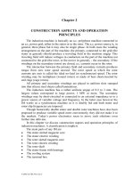
Another implicit problem with convergence is that the objective function
may have multiple maxima (minima) and the optimization method gets trapped
in a local rather than the global optimum (Figure 18.2).
It is only intuitive that, in order to reduce the computation time and increase
the probability of reaching a global optimum, the search in the subspace of
design variables has to be thorough.
global optimum
local optima

Figure 18.2 Multiple maxima objective function for 2 design variables
This process gets simplified if the number of design variables is reduced.
This may be done by intelligently using the constraints in the process. In other
words, the analysis model has to be wisely manipulated to reduce the number of
variables.
It is also possible to start the optimization design with a few different sets of
design variable vectors, within their existence domain. If the final objective
function value is the same for the same final design variables and constraint
violation rate, then the optimization method is able to find the global optimum.
But there is no guarantee that such a happy ending will take place for other
IM with different specifications, investigated with same optimization method.
These challenges have led to numerous optimization method proposals for
the design of electrical machines, IMs in particular.
© 2002 by CRC Press LLC
Author: Ion Boldea, S.A.Nasar………… ………




18.2. ESSENTIAL OPTIMIZATION DESIGN METHODS
Most optimization design techniques employ nonlinear programing (NLP)
methods. A typical form for a uni-objective NLP problem can be expressed in
the form

()
xFminimize
(18.1)

()

ej
1 mj ;0xg
: tosubject
==
(18.2)

(
)
m, ,1mj ;0xg
ej
+=≥
(18.3)

highlow
XXX ≤≤
(18.4)
where
{
}
n11
x, ,x,xX =
(18.5)
is the design variable vector, F(x) is the objective function and g
j
(x) are the
equality and inequality constraints. The design variable vector X is bounded by
lower (X
low
) and upper (X
high

) limits.
The nonlinear programming (NLP) problems may be solved by direct
methods (DM) and indirect methods (IDM). The DM deals directly with the
constraints problem into a simpler, unconstrained problem by integrating the
constraints into an augmented objective function.
Among the direct methods, the complex method [2] stands out as an
extension of the simplex method. [3] It is basically a stochastic approach. From
the numerous indirect methods, we mention first the sequential quadratic
programming (SQP). [4,5] In essence, the optimum is sought by successively
solving quadratic programming (QP) subproblems which are produced by
quadratic approximations of the Lagrangian function.
The QP is used to find the search direction as part of a line search
procedure. Under the name of “augmented Lagrangian multiplies method”
(ALMM) [6], it has been adopted for inequality constraints. Objective function
and constraints gradients must be calculated.
The Hooke–Jeeves [7,8] direct search method may be applied in
conjunction with SUMT (segmented unconstrained minimization technique) [8]
or without it. No gradients are required. Given the large number of design
variables, the problem nonlinearity, the multitude of constraints has ruled out
many other general optimization techniques such as grid search, mapping
linearization, simulated annealing, when optimization design of the IM is
concerned.
Among the stochastic (evolutionary) practical methods for IM optimization
design the genetic algorithms (GA) method [9] and the Montecarlo approach
[10] have gained most attention.
© 2002 by CRC Press LLC
Author: Ion Boldea, S.A.Nasar………… ………

Finally, a fuzzy artificial experience-based approach to optimization design
of double cage IM is mentioned here. [11]
Evolutionary methods start with a few vectors of design variables (initial
population) and use genetics inspired operations such as selection
(reproduction) crossover and mutation to approach the highest fitness
chromosomes by the survival of the fittest principle.
Such optimization approaches tend to find the global optimum but for a
larger computation time (slower convergence). They do not need the
computation of the gradients of the fitness function and constraints. Nor do they
require an already good initial design variable set as most nongradient
deterministic methods do.
No single optimization method has gained absolute dominance so far and
stochastic and deterministic methods have complimentary merits. So it seems
that the combination of the two is the way of the future. First, the GA is used to
yield in a few generations a rough global optimization. After that, ALMM or
Hooke–Jeeves methods may be used to secure faster convergence and larger
precision in constraints meeting.
The direct method called the complex (random search) method is also
claimed to produce good results. [12] A feasible initial set of design variables is
necessary, but no penalty (wall) functions are required as the stochastic search
principle is used. The method is less probable to land on a local optimum due to
the random search approach applied.
18.3. THE AUGMENTED LAGRANGIAN MULTIPLIER METHOD
(ALMM)
To account for constraints, in ALMM, the augmented objective function
L(x,r,h) takes the form

( ) () ()
()

[]
∑
=
++=
m
1i
2
ii
r/hXg,0minrXFh,r,XL
(18.6)
where X is the design variable vector, g
i
(s) is the constraint vector (18.2)–
(18.3), h
(i)
is the multiplier vector having components for all m constraints; r is
the penalty factor with an adjustable value along the optimization cycle.
An initial value of design variables set (vector X
0
) and of penalty factor r
are required. The initial values of the multiplier vector h
0
components are all
considered as zero.
As the process advances, r is increased.

42C ;rCr
k1k
÷=⋅=
+

(18.7)
Also a large initial value of the maximum constraint error is set. With these
initial settings, based on an optimization method, a new vector of design
variables X
k
which minimizes L(X,r,h) is found. A maximum constraint error δ
k

is found for the most negative constraint function g
i
(X).
© 2002 by CRC Press LLC
Author: Ion Boldea, S.A.Nasar………… ………





()
[]
ki
mi1
k
Xg,0minmax
≤≤
=δ
(18.8)
The large value of δ
0
was chosen such that δ

1
< δ
0
. With the same value of
the multiplier, h
(i)k
is set to

()
(
)
()
[
]
1kikik
mi1
ki
hXgr,0minh
−
≤≤
+=
(18.9)
to obtain h
i(1)
. The minimization process is then repeated.
The multiplier vector is reset as long as the iterative process yields a 4/1
reduction of the error δ
k
. If δ
k

fails to decrease the penalty factor, r
k
is increased.
It is claimed that ALMM converges well and that even an infeasible initial X
0
is
acceptable. Several starting (initial) X
0
sets are to be used to check the reaching
of the global (and not a local) optimum.
18.4. SEQUENTIAL UNCONSTRAINED MINIMIZATION
In general, the induction motor design contains not only real but also integer
(slot number, conductor/coil) variables. The problem can be treated as a
multivariable nonlinear programming problem if the integer variables are taken
as continuously variable quantities. At the end of the optimization process, they
are rounded off to their closest integer feasible values. Sequential quadratic
programming (SQP) is a gradient method. [4, 5] In SQP, SQ subproblems are
successively solved based on quadratic approximations of Lagrangian function.
Thus, a search direction (for one variable) is found as part of the line search
procedure. SQP has some distinctive merits.
• It does not require a feasible initial design variable vector
•
Analytical expressions for the gradients of the objective functions or
constraints are not needed. The quadratic approximations of the Lagrangian
function along each variable direction provides for easy gradient
calculations.

To terminate the optimization process there are quite a few procedures:
• Limited changes in the objective function with successive iterations;
• Maximum acceptable constraint violation;

• Limited change in design variables with successive iterations;
• A given maximum number of iterations is specified.

One or more of them may in fact be applied to terminate the optimization
process.
The objective function is also augmented to include the constraints as

() () ()
∑
=
><γ+=
m
1i
2
i
XgXfX'f
(18.10)
where γ is again the penalty factor and
© 2002 by CRC Press LLC
Author: Ion Boldea, S.A.Nasar………… ………





()
() ()
()




<
≥
>=<
0Xg if 0
0Xg if Xg
Xg
i
ii
i
(18.11)
As in (18.7), the penalty factor increases when the iterative process
advances.
The minimizing point of f’(X) may be found by using the univariate method
of minimizing steps. [13] The design variables change in each iteration as:

jjj1j
SXX α+=
+
(18.12)
where S
j
are unit vectors with one nonzero element. S
1
= (1, 0, …,0); S
2
= (0, 1,
…,0) etc.
The coefficient α
j

is chosen such that

(
)
(
)
j1j
XfX'f <
+
(18.13)
To find the best
α,
we may use a quadratic equation in each point.

(
)
(
)
2
cbaHX'f α+α+=α=α+
(18.14)
H(α) is calculated for three values of α,

arbitrary) is (d ,d2 ,d ,0
321
=α=α=α


(
)

()
()
2
3
2
2
1
cd4bd2atd2H
cdbdatdH
at0H
++==
++==
==
(18.15)
From (18.15), a, b, c are calculated. But from

c2
b
;0
H
opt
−
=α=
α∂
∂
(18.16)

d
t2t3t4
tt3t4

132
312
opt
−−
−−
=α
(18.17)
To be sure that the extreme is a minimum,

d2t t;0c
H
13
2
2
>+>=
α∂
∂
(18.18)
These simple calculations have to be done for each iteration and along each
design variable direction.



© 2002 by CRC Press LLC
Author: Ion Boldea, S.A.Nasar………… ………




18.5. A MODIFIED HOOKE–JEEVES METHOD

A direct search method may be used in conjunction with the pattern search
of Hooke-Jeeves. [7] Pattern search relies on evaluating the objective function
for a sequence of points (within the feasible region). By comparisons, the
optimum value is chosen. A point in a pattern search is accepted as a new point
if the objective function has a better value than in the previous point.
Let us denote

()
()
()
move)pattern (after thepoint atternpX
pointy explorator base urrentcX
point base previousX
1k
k
1k
−
−
−
+
−

The process includes exploratory and pattern moves. In an exploratory
move, for a given step size (which may vary during the search), the exploration
starts from X
(k-1)
along each coordinate (variable) direction.
Both positive and negative directions are explored. From these three points,
the best X
(k)

is chosen. When all n variables (coordinates) are explored, the
exploratory move is completed. The resulting point is called the current base
point X
(k)
.
A pattern move refers to a move along the direction from the previous to the
current base point. A new pattern point is calculated

( ) () () ( )
()
1kkk1k
XXaXX
−+
−+=
(18.19)
a is an accelerating factor.
A second pattern move is initiated.

() () () ()
()
k1k1k2k
XXaXX −+=
+++
(18.20)
The success of this second pattern move X
(k+2)
is checked. If the result of
this pattern move is better than that of point X
(k+1)
, then X

(k+2)
is accepted as the
new base point. If not, then X
(k+1)
constitutes the new current base point.
A new exploratory-pattern cycle begins but with a smaller step search and
the process stops when the step size becomes sufficiently small.
The search algorithm may be summarized as
Step 1: Define the starting point X
(k-1)
in the feasible region and start with a
large step size;
Step 2: Perform exploratory moves in all coordinates to find the current base
point X
(k)
;
Step 3: Perform a pattern move:
( ) () () ( )
()
1kkk1k
XXaXX
−+
−+=
with a < 1;
Step 4: Set X
(k-1)
= X
(k)
;
Step 5: Perform tests to check if an improvement took place. Is X

(k+1)
a better
point?
If “YES”, set X
(k)
= X
(k+1)
and go to step 3.
If “NO”, continue;
© 2002 by CRC Press LLC
Author: Ion Boldea, S.A.Nasar………… ………




Step 6: Is the current step size the smallest?
If “YES”, stop with X
(k)
as the optimal vector of variables.
If “NO”, reduce the step size and go to step 2.
To account for the constraints, the augmented objective function f’(X),
(8.10 – 8.11) – is used. This way the optimization problem becomes an
unconstraint one. In all nonevolutionary methods presented so far, it is
necessary to do a few runs for different initial variable vectors to make sure that
a global optimum is obtained. It is necessary to have a feasible initial variable
vector. This requires some experience from the designer. Comparisons between
the above methods reveal that the sequential unconstrained minimization
method (Han & Powell) is a very powerful but time consuming tool while the
modified Hooke–Jeeves method is much less time consuming. [14, 15, 16]
18.6. GENETIC ALGORITHMS

Genetic algorithms (GA) are computational models which emulate
biological evolutionary theories to solve optimization problems. The design
variables are grouped in finite length strings called chromosomes. GA maps the
problem to a set of strings (chromosomes) called population. An initial
population is adopted by way of a number of chromosomes. Each string
(chromosome) may constitute a potential solution to the optimization problem.
The string (chromosome) can be constituted with an orderly alignment of
binary or real coded variables of the system. The chromosome−the set of design
variables – is composed of genes which may take a number of values called
alleles. The choice of the coding type, binary or real, depends on the number
and type of variables (real or integer) and the required precision. Each design
variable (gene) is allowed a range of feasible values called search space. In GA,
the objective function is called fitness value. Each string (chromosome) of
population of generation i, is characterised by a fitness value.
The GA manipulates upon the population of strings in each generation to
help the fittest survive and thus, in a limited number of generations, obtain the
optimal solution (string or set of design variables). This genetic manipulation
involves copying the fittest string (elitism) and swapping genes in some other
strings of variables (genes).
Simplicity of operation and the power of effect are the essential merits of
GA. On top of that, they do not need any calculation of gradients (of fitness
function) and provide more probably the global rather than a local optimum.
They do so because they start with a random population–a number of
strings of variables–and not only with a single set of variables as
nonevolutionary methods do.
However their convergence tends to be slow and their precision is
moderate. Handling the constraints may be done as for nonevolutionary
methods through an augmented fitness function.
Finally, multi-objective optimization may be handled mainly by defining a
comprehensive fitness function incorporating as linear combinations (for

example) the individual fitness functions.
© 2002 by CRC Press LLC
Author: Ion Boldea, S.A.Nasar………… ………




Though the original GAs make use of binary coding of variables, real coded
variables seem more practical for induction motor optimization as most
variables are continuous. Also, in a hybrid optimization method, mixing GAs
with a nonevolutionary method for better convergence, precision, and less
computation time, requires real coded variables.
For simplicity, we will refer here to binary coding of variables. That is, we
describe first a basic GA algorithm.
A simple GA uses three genetic operations:
• Reproduction (evolution and selection)
• Crossover
• Mutation
18.6.1. Reproduction (evolution and selection)
Reproduction is a process in which individual strings (chromosomes) are
copied into a new generation according to their fitness (or scaled fitness) value.
Again, the fitness function is the objective function (value).
Strings with higher fitness value have a higher probability of contributing
one or more offsprings in the new generation. As expected, the reproduction
rate of strings may be established, many ways.
A typical method emulates the biased roulette wheel where each string has a
roulette slot size proportional to its fitness value.
Let us consider as an example 4 five binary digit numbers whose fitness
value is the decimal number value (Table 18.1).
Table 18.1.

String number String Fitness value % of total fitness
value
1 01000 64 5.5
2 01101 469 14.4
3 10011 361 30.9
4 11000 576 49.2
Total 1170 100

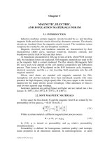
The percentage in Table 18.1 may be used to draw the corresponding biased
roulette wheel (Figure 18.2).
Each time a new offspring is required, a simple spin of the biased roulette
produces the reproduction candidate. Once a string has been selected for
reproduction, an exact replica is made and introduced into the mating pool for
the purpose of creating a new population (generation) of strings with better
performance.

© 2002 by CRC Press LLC
Author: Ion Boldea, S.A.Nasar………… ………




30.9%
14.4%
5.5%
49.2%

Figure 18.3 The biased roulette wheel
The biased roulette rule of reproduction might not be fair enough in
reproducing strings with very high fitness value. This is why other methods of

selection may be used. The selection by the arrangement method for example,
takes into consideration the diversity of individuals (strings) in a population
(generation). First, the m individuals are arranged in the decreasing order of
their fitness in m rows.
Then the probability of selection ρ
i
as offspring of one individual situated in
row i is [1]

(
)
(
)
(
)
[]
m
1m/221r
i
i
−−φ−−φ
=ρ
(18.21)
φ – pressure of selection φ = (1 – 2);
m – population size (number of strings);
r
i
– row of i
th
individual (there are m rows);

ρ
i
– probability of selection of i
th
row (individual).
Figure 18.4 shows the average number of offspring versus the row of
individuals. The pressure of selection φ is the average number of offspring of
best individual. For the worst, it will be 2 – φ. As expected, an integer number
of offspring is adopted.
123 m-1m
2-
φ
1
φ
ρ

Figure 18.4 Selection by arrangement
© 2002 by CRC Press LLC
Author: Ion Boldea, S.A.Nasar………… ………




By the pressure of selection φ value, the survival chance of best individuals
may be increased as desired.
18.6.2. Crossover
After the reproduction process is done crossover may proceed. A simple
crossover contains two steps:
•
Choosing randomly two individuals (strings) for mating

• Mating by selection of a crossover point K along the chromosome length l.
Two new strings are created by swapping all characters in positions K + 1
to l (Figure 18.5).
Besides simple (random) crossover, at the other end of scale, completely
continued crossover may be used. Let us consider two individuals of the t
th

generation A(t) and B(t), whose genes are real variables a
1
, …, a
n
and b
1
, …, b
n
,

()
[]
n21
a, ,a,atA =
(18.22)

()
[]
n21
b, ,b,btB =
(18.23)
The two new offspring A(t+1) and B(t+1) may be produced by linear
combination of parents A(t) and B(t).

crossover point
0
1
1
0
1
1
1
0
0
0
Two old
chromosomes
crossover
0
1
1
0
0
no1'
1
1
0
0
1
no2'
Two new
chromosomes
no1 no2

Figure 18.5 Simple crossover operation

() ( ) ( )
[]
nnnn1111
b1a, ,b1a1tA ρ−+ρρ−+ρ=+
(18.24)

() ( ) ( )
[]
nnnn1111
a1b, ,a1b1tB ρ−+ρρ−+ρ=+
(18.25)
where ρ
1
, …, ρ
n
∈ [0,1] are random values (uniform probability distribution).
18.6.3. Mutation
Mutation is required because reproduction and crossover tend to become
overzealous and thus lose some potentially good “genetic material”.
In simple GAs, mutation is a low probability (occasional) random alteration
of one or more genes in one or more offspring chromosomes. In binary coding
© 2002 by CRC Press LLC
Author: Ion Boldea, S.A.Nasar………… ………




GAs, a zero is changed to a 1. The mutation plays a secondary role and its

frequency is really low.
Table 18.2 gives a summary of simple GAs.
Table 18.2. GA stages
Stage Chromosomes Fitness value
Initial population:
(size 3, with 8
genes and its fitness values)
P
1
: 11010110
P
2
: 10010111
P
3
: 01001001
F(P
1
) = 6%
F(P
2
) = 60%
F(P
3
) = 30%
Reproduction:
based on fitness
value a number of chromosomes
survive. There will be two P
2

and
one P
3
.
P
2
: 10010111
P
2
: 10010111
←
|
→

P
3
: 01001001
no need to recalculate fitness as
P
2
and P
3
will mate
Crossover:
some portion of P
2
and
P
3
will be swapped

P
2
: 10010111
P
2
’: 10010001
P
3
’: 01001111
no need of it here
Mutation:
some binary genes of
some chromosomes are inverted
P
2
: 10010111
P
2
”: 1001
1
001
P
3
’: 01001111
A new generation of individuals
has been formed; a new cycle
starts

In real coded GAs, the mutation changes the parameters of selected
individuals by a random change in predefined zones. If A(t) is an individual of

t
th
generation, subject to mutation, each gene will undergo important changes in
first generations. Gradually, the rate of change diminishes. For the t
th

generation, let us define two numbers (p) and (r) which are randomly used with
equal probabilities.

ondistributi uniform [0,1]r
alteration negative -1p
alteration positive 1p
−∈
−=
−+=
(18.26)
The factor r selected for uniform distribution determines the amplitude of
change. The mutated (K
th
) parameter (gene) is given by [18]

()
()
1pfor ;r1aaa'a
1pfor ;r1aaa'a
5
5
T
t
1

kminkkk
T
t
1
kkmaxkk
−=










−−−=
+=










−−+=







−






−
(18.27)
a
kmax
and a
kmin
are the maximum and minimum feasible values of a
k
parameter
(gene).
T is the generation index when mutation is cancelled. Figure 18.6 shows the
mutation relative amplitude for various generations (t/T varies) as a function of
the random number r, based on (18.27).
© 2002 by CRC Press LLC
Author: Ion Boldea, S.A.Nasar………… ………

1
0.5
0.5 1
t/T=0
t/T=0.25
t/T=0.5
random r
(1-r )
(1-t/T)
5

Figure 18.6 Mutation amplitude for various generations (t/T)
18.6.4. GA performance indices
As expected, GAs are supposed to produce a global optimum with a limited
number (%) of all feasible chromosomes (variable sets) searched. It is not easy
to assess the minimum number of generations (T) or the population size (m)
required to secure a sound optimal selection. The problem is still open but a few
attempts to solve it have been made.
A schema, as defined by Holland, is a similarity template describing a
subset of strings with similarities at certain string positions.
If to a binary alphabet {0,1} we add a new symbol * which may be
indifferent, a ternary alphabet is created {1,0,*}.
A subset of 4 members of a schema like *111* is shown in (18.28).

{}
1100,01111,0111111,1111
(18.28)
The length of the string n
1

= 5 and thus the number of possible schemata is
3
5
. In general, if the ordinality of the alphabet is K (K = 2 in our case), there are
(K + 1)
n
schemata.
The exact number of unique schemata in a given population is not countable
because we do not know all the strings in this particular population. But a bound
for this is feasible.
A particular binary string contains
1
n
2
schemata as each position may take
its value or * thus a population of size m contains between
1
n
2
and m⋅
1
n
2

schemata. How many of them are usefully processed in a GA? To answer this
question, let us introduce two concepts.
• The order o of a schema H (δ(H)): the number of fixed positions in the
template. For 011**1**, the order o(H) is 4.
• The length of a schema H, (δ(H)): the distance between the first and the last
specified string position. In 011**1**, δ(H) = 6 – 1 = 5.

© 2002 by CRC Press LLC
Author: Ion Boldea, S.A.Nasar………… ………




The key issue now is to estimate the effect of reproduction, crossover and
mutation on the number of schemata processed in a simple GA.
It has been shown [9] that short, low order, above-average fitness schemata
receive exponentially increasing chances of survival in subsequent generations.
This is the fundamental theorem of GAs.
Despite the disruption of long, high-order schemata by crossover and
mutation, the GA implicitly process a large number of schemata (%n
1
3
) while in
fact they explicitly process a relatively small number of strings (m in each
population). So, despite the processing n
1
of structures, each generation GAs
process approximately n
1
3
schemata in parallel with no memory of bookkeeping.
This property is called implicit parallelism of computation power in GAs.
To be efficient, GAs must find solutions by exploring only a few
combinations in the variable search space. Those solutions must be found with a
better probability of success than with random search algorithms. The traditional
performance criterion of GA is the evolution of average fitness of the
population through subsequent generations.

It is almost evident that such a criterion is not complete as it may
concentrate the point around a local, rather than global optimum.
A more complete performance criterion could be the ratio between the
number of success runs per total given number of runs (1000 for example, [19],
P
ag
(A)):

()
1000
runs success ofnumber
AP
ag
= (18.29)
For a pure random search algorithm, it may be proved that the theoretical
probability to find p optima in a searching space of M possible combinations,
after making A% calls of the objective functions, is [19]

()
∑
=
−
⋅=






−=

K
1i
1i
rand
1000
M
K
A ;
M
p
1
M
p
AP
(18.30)
The initial population size M in GA is generally M > 50.
We should note that when the searching space is discretised the number of
optima may be different than the case of continuous searching space.
In general, the crossover probability P
c
= 0.7 and the mutation probability
P
m
≤ 0.005 in practical GAs. For a good GA algorithm, searching less than A =
10% of the total searching space should produce a probability of success P
ag
(A)
> P
rand
(A) with P

ag
(A) > 0.8 for A = 10% and P
ag
(A) > 0.98 for A = 20%.
Special selection mechanisms, different from the biased roulette wheel
selection are required. Stochastic remainder techniques [17] assign offsprings to
strings based on the integer part of the expected number of offspring. Even such
solutions are not capable to produce performance as stated above.
However if the elitist strategy is used to make sure that the best strings
(chromosomes) survive intact in the next generation, together with selection by
© 2002 by CRC Press LLC
Author: Ion Boldea, S.A.Nasar………… ………




stochastic remainder technique and real coding, the probability of success may
be drastically increased. [19]
Recently the GAs and some deterministic optimization methods have been
compared in IM design [20−23]. Mixed conclusions have resulted. They are
summarized below.
18.7. SUMMARY
• GAs offer some advantages over deterministic methods.
• GAs reduce the risk of being trapped in local optima.
• GAs do not need a good starting point as they start with a population of
possible solutions. However a good initial population reduces the
computation time.
• GAs are more time consuming though using real coding, elitist strategy and
stochastic remainder selection techniques increases the probability of
success to more than 90% with only 10% of searching space investigated.

• GAs do not need to calculate the gradient of the fitness function; the
constraints may be introduced in an augmented fitness function as penalty
function as done with deterministic methods. Many deterministic methods
do not require computation of gradients.
• GAs show in general lower precision and slower convergence than
deterministic methods.
• Other refinements such as scaling the fitness function might help in the
selection process of GAs and thus reduce the computation time for
convergence.
• It seems that hybrid approaches which start with GAs (with real coding), to
avoid trapping in local optima and continue with deterministic (even
gradient) methods for fast and accurate convergence, might become the
way of the future.
•
If a good initial design is available, optimization methods produce only
incremental improvements; however, for new designs (high speed IMs for
example), they may prove indispensable.
• Once optimization design is performed based on nonlinear analytical IM
models, with frequency effects approximately considered, the final solution
(design) performance may be calculated more precisely by FEM as
explained in previous chapters.
• For IM with involved rotor slot configurations – deep bars, closed slots,
double-cage – it is also possible to leave the stator unchanged after
optimization and change only the main rotor slot dimensions (variables) and
explore by FEM their effect on performance and constraints (starting
torque, starting current) until a practical optimum is reached.
• Any optimization approach may be suited to match the FEM. In [14], a
successful attempt with Fuzzy Logic optimiser and FEM assistance is
presented for a double-cage IM. Only a few tens of 2DFEM runs are used
and thus the computation time remains practical.

© 2002 by CRC Press LLC
Author: Ion Boldea, S.A.Nasar………… ………




• Notable advances in matching FEM with optimization design methods are
expected as the processing power of PCs is continuously increasing.
18.8. REFERENCES
1. U. Sinha, A Design and Optimization Assistant for Induction Motors and
Generators, Ph.D. Thesis, MIT, June 1998.
2. M.Box, A New Method of Constrained Optimization and a Comparison
With Other Methods, Computer Journal, Vol.8, 1965, pp.42–52.
3. J. Helder, R. Mead, A Simplex Method for Function Minimization,
Computer Journal, Vol.7, 1964, pp.308 – 313.
4. S.P. Han, A Globally Convergent Method for Nonlinear Programming,
Journal of optimization theory and applications”, Vol22., 1977, pp.297 –
309.
5. M.J.D. Powell, A Fast Algorithm for Nonlinearly Constrained Optimization
Calculation, Numerical Analysis, Editor: D.A.Watson, Lecture notes in
mathematics, Springer Verlag, 630, 1978, pp.144 – 157.
6. R. Rockafeller, Augmented Lagrange Multiplier Functions and Duality in
Convex Programming, SIAM, J.Control, Vol.12, 1994, pp.268 – 285.
7. R. Hooke, T.A. Jeeves, Direct Search Solution of Numerical and Statistical
Problem, Journal of ACM, Vol.8, 1961, pp.212.
8. R. Ramarathnam, B.G. Desa, V.S. Rao, A Comparative Study of
Minimization Techniques for Optimization of IM Design, IEEE Trans.
Vol.PAS – 92, 1973, pp.1448 – 1454.
9. D.E. Goldberg, Genetic Algorithms in Search Optimization and Machine
Learning, Addison Wesley Longman Inc., 1989.

10. U. Sinha, A Design Assistant for Induction Motors, S.M.Thesis,
Department of Mechanical Engineering, MIT, August, 1993.
11. N. Bianchi, S. Bolognani, M. Zigliotto, Optimised Design of a Double Cage
Induction Motor by Fuzzy Artificial Experience and Finite Element
Analysis, Record of ICEM – 1998, Vol.1/3.
12. Q. Changtoo, Wu Yaguang, Optimization Design of Electrical Machines by
Random Search Approach, Record of ICEM – 1994, Paris, session D16,
pp.225 – 229.
13. A.V. Fiacco, G.P. McCormick, Nonlinear Programming Sequential
Unconstrained Minimization Techniques, John Wiley, 1969.
14. J. Appelbaum, E.F. Fuchs, J.C. White, I.A. Kahn, Optimization of Three
Phase Induction Motor Design, Part I + II, IEEE Trans. Vol. EC – 2, No.3,
1987, pp.407 – 422.
15. Ch. Li, A. Rahman, Three–phase Induction Motor Design Optimization
Using The Modified Hooke–Jeeves Method, EMPS Vol.18, No.1, 1990,
pp.1 – 12.
16. C. Singh, D. Sarkas, Practical Considerations in the Optimization of
Induction Motor Design, Proc.IEE, Vol.B – 149, No.4, 1992, pp.365 – 373.
17. J.E. Baker, Adaptive Selection Methods of Genetic Algorithms, Proc. of the
first International Conference on Genetic Algorithms, 1998, pp.101 – 111.
© 2002 by CRC Press LLC
Author: Ion Boldea, S.A.Nasar………… ………




18. C.Z. Janikov, Z. Michaleewiez, An Experimental Comparison of Binary
and Floating Point Representation in Genetic Algorithms, Proc. of Fourth
International Conference on Genetic Algorithms, 1991, pp.31 – 36.
19. F. Wurtz, M. Richomme, J. Bigeon, J.C. Sabonnadiere, A few Results for

Using Genetic Algorithms in the Design of Electrical Machines, IEEE
Trans., Vol.MAG – 33, No.2, 1997, pp.1892 – 1895.
20. M. Srinivas, L.M. Patniak, Genetic Algorithms: A Survey, in Computer, an
IEEE review, June 1994, pp.17 – 26.
21. S. Hamarat, K. Leblebicioglu, H.B. Ertan, Comparison of Deterministic and
Nondeterministic Optimization Algorithms for Design Optimization of
Electrical Machines, Record of ICEM – 1998, pp.1477 – 1481.
22. Ö. Göl, J.P. Wieczorek, A Comparison of Deterministic and Stochastic
Optimization Methods in Induction Motor Design, IBID, pp.1472 – 1476.
23. S.H. Shahalami, S. Saadate, Genetic Algorithm Approach in the
Identification of Squirrel Cage Induction Motor’s Parameters, Record of
ICEM – 1998, pp.908 – 913.

© 2002 by CRC Press LLC