variable speed generatorsch (13)
Bạn đang xem bản rút gọn của tài liệu. Xem và tải ngay bản đầy đủ của tài liệu tại đây (7.35 MB, 40 trang )
© 2006 by Taylor & Francis Group, LLC
12-1
12
Linear Motion
Alternators (LMAs)
12.1 Introduction 12-1
12.2 LMA Principle of Operation
12-2
The Motion Equation
12.3 PM-LMA with Coil Mover 12-6
12.4 Multipole LMA with Coil Plus Iron Mover
12-7
12.5 PM-Mover LMAs
12-13
12.6 The Tubular Homopolar PM Mover
Single-Coil LMA
12-16
12.7 The Flux Reversal LMA with Mover
PM Flux Concentration
12-20
12.8 PM-LMAs with Iron Mover
12-27
12.9 The Flux Reversal PM-LMA Tubular
Configuration
12-27
The Analytical Model
12.10 Control of PM-LMAs 12-32
Electrical Control • The Spark-Ignited Gasoline Linear
Engine Model • Note on Stirling Engine LMA Stability
12.11 Progressive-Motion LMAs for Maglevs
with Active Guideway
12-35
Note on Magnetohydrodynamic (MHD) Linear
Generators
12.12 Summary 12-39
References
12-40
12.1 Introduction
This chapter deals mainly with linear oscillatory motion electric generators. The linear excursion is within
a few centimeters. As prime movers, free piston Stirling engines (SEs), linear internal combustion single-
piston engines, and direct wave energy engines (with meter range excursions) are proposed.
So far, the Stirling engine [1] has been used for spacecraft and for residential electric energy generation
electric vehicles.
While rotary motion electric generators are multiphase machines, in general, the linear motion alter-
nators (LMAs) tend to be single-phase machines, because the linear oscillatory motion imposes a change
of phase sequence for change in the direction of motion. A three-phase LMA may be built of three single-
phase LMAs.
(Figure 12.1) [1]. The linear internal combustion engine (ICE) was recently proposed for series hybrid
© 2006 by Taylor & Francis Group, LLC
12-2 Variable Speed Generators
Though at first LMAs with electromagnetic excitation were proposed as single-phase synchronous
generators (SGs), more recently, permanent magnet (PM) excitation took over, and most competitive
LMAs now rely on PMs.
A brief classification into three categories may be useful:
• With coil mover (and stator PMs)
• With PM mover
• With iron mover (and stator PMs)
One configuration in each category is treated separately in terms of principle and performance equations.
The dynamics and control will be treated once for all configurations. A special kind of linear motion
generator with progressive motion to provide on-board energy on maglev (magnetically levitated) vehi-
cles with active guideway is also briefly discussed.
12.2 LMA Principle of Operation
PM-LMAs with oscillatory motion are, generally, single-phase machines with harmonic motion:
(12.1)
The electromagnetic force (emf) is, in general,
(12.2)
where is the PM flux linkage in the phase coils.
With Equation 12.1 in Equation 12.2,
(12.3)
To obtain a sinusoidal emf waveform, Equation 12.3 yields the following:
(12.4)
FIGURE 12.1 Stirling engine — linear alternator.
Heater
Regenerator
Cooler
Alternator
Piston
Cold space
Displacer rod (area A
d
)
Gas spring
(pressure P
d
)
Bounce space
Displacer
Hot space
Cylinder (area A)
P
0
x
p
x
d
V
c
V
c
T
c
p
P
1
T
hr
xx t
mr
= sin
ω
et
x
dx
dt
PM
()=−
∂
∂
Ψ
Ψ
PM
et
x
xt
PM
mr r
() sin=−
∂
∂
Ψ
ωω
∂
∂
=
Ψ
PM
e
x
C
© 2006 by Taylor & Francis Group, LLC
Linear Motion Alternators (LMAs) 12-3
This means that the PM flux linkage in the phase coils has to vary linearly with mover position. Flux
reversal is most adequate for the scope (Figure 12.2a and Figure 12.2b).
The excursion length is 2
x
m
but x varies sinusoidally between x
m
and −x
m
.
The ideal harmonic linear motion and PM flux linkage linear variation with mover position are met
only approximately in practice.
In essence, the (
x) flattens toward excursion ends (Figure 12.2b), which leads to the presence of
third, fifth, and seventh harmonics in Also, mainly due to magnetic saturation variation with
instantaneous current and mover position, even harmonics (second and fourth) may occur in
Through finite element method (FEM), the emf harmonics content for harmonic motion may be fully
elucidated. The electromagnetic force is as follows:
(12.5)
Ideally, with the trust varies as the current does.
The highest interaction electromagnetic force per given current occurs (Equation 12.5) when the
and are in phase with each other.
For constant, from Equation 12.4, it follows that
e(t) is in phase with the linear speed. So,
for highest trust/current, the current has to also be in phase with the linear speed.
The above rationale is valid if the phase inductance is independent of mover position, that is, if the
reluctance trust is zero.
In the presence of PMs, a cogging force, occurs for zero current. This force, if existent, should be
zero for the mover in the middle position and maximum at excursion ends, in order to behave like a
“magnetic spring” and, thus, be useful in the energy conversion
For the ideal LMA, with harmonic motion,
(provided by the regulated prime mover), and perfectly linear cogging force characteristic, under steady
state, the voltage equation is, in complex variables,
(12.6)
with
(12.7)
The phase voltage of the power grid is phase shifted by the voltage power angle with respect to
the emf
FIGURE 12.2 Permanent magnet (PM) flux linkage vs. mover position: (a) ideal and (b) real.
Extreme
left
Extreme
right
(a) (b)
X(position)
X
m
−X
m
Ψ
PMax
Ψ
PM
−Ψ
PMax
X(position)
X
m
−X
m
Ψ
PM
Ψ
PM
et().
et().
Ft
e
()
Ft
et it
x
it
e
dx
dt
PM
()
() ()
()=
⋅
=−
∂
∂
Ψ
d
dx
e
PM
C
Ψ
= ,
et() it()
ddx
PM
Ψ / =
L
s
F
r
F
cog
,
()FK
cog cog
≈−
Lconst
s
= , et E t
mr
() cos ,=
ω
ECx
memr
=⋅⋅
ω
xx t
mr
= sin
ω
VRjLIE
srs
1
11
=− + +()
ω
EEe VVe
m
jw
r
t
jt
rv
1
1
1
2==
−()
ωδ
V
1
δ
V
E
1
.
⋅x(Figure 12.3).
© 2006 by Taylor & Francis Group, LLC
12-4 Variable Speed Generators
The phasor diagram of Equation 12.6 and Equation 12.7 is shown in Figure 12.4 for the general case
when is not in phase in The operation is similar to that for an SG, although a single-phase one.
The delivered power is as follows:
(12.8)
The delivered active average power is
(12.9)
To deliver power to a power grid of voltage (root mean squared [RMS] value), the RMS value of
emf should be considerably larger than the former:
(12.10)
due to the inductance and resistance voltage drop. A series capacitor may be used to compensate
for these voltage drops, at least partially. The power pulsates with double-source frequency as for
any single-phase source.
We considered from the start that the frequency of the power grid voltage is the same, as that
of the emf, given by the harmonic motion (Equation 12.1 through Equation 12.3).
FIGURE 12.3 The prime mover and linear motion alternator (LMA) system.
FIGURE 12.4 Phasor diagram of linear motion alternator (LMA).
Prime mover
LMA stator
LMA mover
Mechanical spring
I
1
E
1
.
S
SVI PjQ=⋅
()
=+
∗
1
1
11
P
1
PalVI
E
IRI
m
s1
1
1
11 1
2
2
=⋅
()
=−
∗
Re cos
δ
V
1
E
m
/ 2
EV
m
>
1
2
L
s
R
s
2
ω
r
,
V
1
ω
r
,
Ψ
PM
d
i
d
V
jw
1
L
s
I
1
j
1
E
1
V
1
− R
s
I
1
I
1
© 2006 by Taylor & Francis Group, LLC
Linear Motion Alternators (LMAs) 12-5
The synchronization process would be similar to the case of rotary synchronous machines, but we
have to regulate the motion amplitude and frequency so as to fulfill the condition of equal frequency
and Subsequently, to load the generator, the motion amplitude has to be increased in order to
increase the delivered power.
The frequency remains constant, as the power grid is considered much stronger than the LMA.
Alternatively, the stand-alone operation of LMA is not constrained in frequency, but the output is
increased by increasing the motion amplitude, below the maximum limit
x
max
.
12.2.1 The Motion Equation
The equation of motion is, essentially, as follows:
(12.11)
The mechanical openings force is
(12.12)
with equal to the total moving mass:
(12.13)
(12.14)
For stead-state harmonic motion, the prime mover should ideally cover only the electromagnetic force
:
(12.15)
Then, to fulfill Equation 12.11, we also need to know that
(12.16)
as it follows that
(12.17)
and finally,
(12.18)
Equation 12.18 spells out the mechanical resonance condition. So, the electrical frequency (equal to the
mechanical one) should be equal to the spring proper frequency.
In this case, the prime mover has to provide only the useful electromagnetic power, while the mechan-
ical springs do the conversion of electrical to kinetic (and back) power at excursion ends, securing the
best efficiency conditions.
If linear, the cogging spring-type force helps the mechanical springs. In reality, the cogging force drops
notably at excursion ends, leading to the nonlinear spring characteristic that limits the maximum stable
motion amplitude to (0.80 to 0.95)
x
m
; x
m
is the ideal maximum motion amplitude (where the flux
linkage is maximum).
Now that the basic principles are elucidated, we may proceed to the first category of LMAs — that
with coil movers and stator PMs.
EV
1
1
= .
m
dx
dt
FFFF
tmececogspring
⋅=−++
2
2
F
spring
FKx
spring
=− ⋅
m
t
FCx
cog cog
=− ⋅
Ft C it
ee
() ()=⋅
F
e
Ft F t
emec
() ()=
m
dx
dt
KC x
tcog
2
2
0++ =()
xx t
mr
= sin ,
ω
−++
(
)
=mx K C x t
tm r cog m r
ωω
2
0()sin
ω
r
cog
t
KC
m
=
+()
Ψ
PM
© 2006 by Taylor & Francis Group, LLC
12-6 Variable Speed Generators
12.3 PM-LMA with Coil Mover
The PM-LMA with coil mover stems from the microphone (and loud speaker) principle (Figure 12.5).
The ring-shaped permanent magnet is placed within a cylindrical space in the airgap. The airgap is
partially filled with the coil mover. The coil mover is made of ring-shaped turns placed in an electrical
insulation keeper that is mechanically rugged enough to withstand large forces. As the coil moves back
and forth axially, the PM field induces an emf in the coil that is proportional to the linear speed the
flux density the average length of the turn, and the number of active turns per PM length
(12.19)
The total number of turns per coil corresponds to the total coil length, which surpasses the PM
length by the stroke length
(12.20)
This means that only part of the coil is active in terms of emf, while the whole coil intervenes with its
resistance and inductance. Alternatively, the PMs may be longer than the coil by the stroke length.
As the motion is considered harmonic, the emf e(t) is sinusoidal, unless magnetic saturation on load
or PM flux fringing influences making it slightly dependent on the mover position.
It should also be noticed that the homopolar character of the PM magnetic field leads to a large
magnetic core of the stator, while the placement of mechanical springs is not an easy task either.
The mechanical rigidity of the coil mover with flexible electrical terminals is not high. On the good
side, the mover weight tends to be low, and the copper use and heat transfer surface are large, allowing
for large current densities and, thus, lower mover size, at the price of larger copper losses.
The average linear speed in LMA is rather low. For example, for speed at = 60 Hz and = 10 mm,
the maximum speed = 0.01 ⋅ 2
π
⋅ 60 = 3.76 m/sec. The average speed = 4 ⋅ 0.01⋅
2
π
⋅ 60 m/sec. For given electromagnetic power, say W, it would mean an average electromag-
netic force = 1200/2.4 = 500 N.
The total magnetic airgap which includes the two mechanical gaps plus the coil radial
height and the PM height is as follows:
(12.21)
FIGURE 12.5 Homopolar linear motion alternator (LMA) with coil mover.
Mechanical
springs
Prime
mover
piston
S
S
a
A
1
stroke
= 2x
m
×××××
Coil-mover
Mild ferrite or magnetic
powder stator core
Ring shape coil in
insulation-keeper mover
Stator ring-shape PM
Α
Ring shape
PM
Stator magnetic
core
A-A
1
PM
N
N
dx dt/ ,
B
gPM
,
′
n
c
l
PM
:
et
dx
dt
nl B
cav PM
av
()=− ⋅
′
⋅⋅
n
c
l
PM
lx
stroke
= 2
max
:
nn
ll
l
cc
stroke PM
PM
=
′
+()
B
PMav
,
f
1
x
m
Ux
mrmax
=
ω
Uxf
av m
= 4
1
P
elm
=1200
FPU
eelmav
av
=
/
h
M
,
g,
h
coil
, h
PM
hh h g h
MPMcoil PM
=++<−2222(.)
© 2006 by Taylor & Francis Group, LLC
Linear Motion Alternators (LMAs) 12-7
The condition in Equation 12.21 preserves large enough PM flux density levels in the airgap with a good
use of PMs.
For larger powers (forces), heteropolar LMA, with multiple coils connected in counter-series or in
antiparallel, may be conceived as multipolar structures (Figure 12.6). As visible in Figure 12.6, the mover
now contains a magnetic core that makes it more rugged, but it adds weight. The rather small pole pitch
of the PM placing makes, however, the thickness of the mover core rather small, in general,
As the actual PM flux density is below and only half of the PM pole flux flows through the back
core, the mover core thickness is, in general, even for T. The larger the , the
better copper utilization will be, but this comes at the price of additional iron in the back cores. An
optimum situation in terms of efficiency, another in terms of costs, and yet another in terms of mover
weight is felt to exist when such a coil mover LMA is designed.
Note that the increase in mover weight poses severe limitations on the frequency of stable oscillatory
of motion by the prime-mover control.
As the homopolar LMA is treated in detail elsewhere [1], we will concentrate here on the multipolar
(heteropolar) LMA with coil plus iron mover.
12.4 Multipole LMA with Coil Plus Iron Mover
mover, is suitable for high-force applications, because as the force increases, both the mover external
diameter and the number of poles
1
may be increased. This is not the case with the homopolar
needed. Also, the force at zero current (cogging force ) and the reluctance force are both zero.
The PM flux distribution and force production may be calculated with precision by two-dimensional
(2D) FEM.
The stator core may be made of solid mild iron, while the mover core below the coils has to be fabricated
from magnetic powders or from ring-shaped thin laminations with a filling factor of 0.95 or more to
allow for large enough PM flux density in the airgap.
Magnetic saturation may be considered a second-order effect, as the coils are placed in air to reduce
the mover weight and also to reduce machine inductance.
An approximate analytical model is always useful for a preliminary investigation. Let us pursue it here.
FIGURE 12.6 Heteropolar (multipolar) permanent magnet linear motion alternator (PM-LMA) with coil mover
in extreme left position.
1
stroke
1
PM
1
PM
/2
Ring shape
multipolar coil
End springs
Solid (or magnetic powder)
cylindrical stator back core
Ring shape PMs
Magnetic powder
mover core
End springs
S
NS
h
er
NSN
NSNS
1
PM
/2
×××× ×××××××××××××
××××××××××××××××××
ll
PM stroke
≈−().12
B
r
/2,
hl
cr PM
≤
/
4, B
r
=12. ll
PM stroke
/
2p
F
cog
()F
r
The tubular configuration in Figure 12.5 that constitutes the multipole LMA with coil plus iron
configuration (Figure 12.3), where only the mover diameter may be increased when more force is
The detailed pole (section) geometry is as shown in Figure 12.7.
© 2006 by Taylor & Francis Group, LLC
12-8 Variable Speed Generators
The airgap PM flux density in the airgap is
, (12.22)
where is the fringing factor that accounts for the PM flux leaking through the airgap and between
neighboring PMs, axially.
The fringing coefficient depends on and on besides the magnetic
saturation in the mover and in the stator back cores.
Though approximate analytical expressions for may be derived, FEM should be used to obtain
reliable information in this matter.
In general, however, for a good design, takes care of magnetic saturation and is
generally less than 0.05 to 0.15 in a well-designed machine.
The emf in the
1
coils in series, E, is as follows:
(12.23)
In Equation 12.23, only the part of the coils under the direct influence of PMs is considered to produce
force, while the total number of turns/coil is is the average coil-turn diameter.
The electromagnetic force is as follows:
(12.24)
The machine inductance and resistance are
(12.25)
FIGURE 12.7 Geometrical details of multipole permanent magnet linear motion alternator (PM-LMA) with coil
plus iron mover.
1
stroke
= 2x
m
1
PM
g
h
PM
h
coil
D
cr
D
cs
h
cs
Fringing flux
Main flux
h
cm
B
gPM
B
Bh
hgh k
gPM
rPM rec
PM coil rec fri
≈
⋅⋅
++ ⋅
⋅
+
µ
µ
()(
1
1
nnge s
K)( )⋅+1
k
fringe
k
fringe
(( ) )1++gh h
coil PM
/ lh
stroke PM
/
,
k
fringe
k
fringe
<−03 05 K
s
2p
Et B Ut D pn
l
ll
gPM avc c
PM
PM stroke
() ()=⋅⋅⋅⋅⋅⋅
+
π
2
nD
cav
;
F
e
Ft B n
l
ll
D
egPMc
PM
PM stroke
avc
()=⋅⋅
+
⋅⋅
π
⋅⋅ ⋅2pit()
L
s
R
s
LpnD
ll
hgh
scavc
PM stroke
PM co
≈⋅ ⋅ ⋅⋅⋅
+
++
1
8
2
0
2
µπ
(
iil
sco avc
c
In
j
RD
np
nc
con
)
()
=⋅⋅ ⋅
⋅
′
ρπ
2
2
© 2006 by Taylor & Francis Group, LLC
Linear Motion Alternators (LMAs) 12-9
where
is the RMS value of rated current
is the rated current density in the design
For forced air cooling, A/mm
2
; otherwise, it is 4 to 6 A/mm
2
. The factor 1/8 comes from
the linear variation of current-produced field with position. The core losses occur mainly in the mover
core, but, at least for electrical frequencies Hz, they are likely to be only a fraction (10 to 15%
at most) of copper losses.
The machine behaves like a single-phase nonsalient-pole PM alternator, and thus, under steady state,
the voltage equation in complex variables is as known (Equation 12.6 and Equation 12.7):
(12.26)
As the stator and mover cores handle half the pole flux, the core depths and are as follows:
(12.27)
The influence of circularity was considered in the mover, because when the mover diameter gets smaller,
the latter has a notable influence.
The coefficient accounts for the increase in flux density due to coil current for the case
when the equals in amplitude This corresponds approximately to a power factor of
(Figure 12.4), which is considered a good compromise between force density and energy conversion
performance:
(12.28)
Example 12.1
Consider a multipolar PM-LMA with coil iron mover and the following specifications:
• Electrical output: kW at V
ac
(RMS)
• Efficiency:
• Load power factor: unity
• Frequency: 60 Hz
• Stroke length (imposed by the prime mover): mm
• Harmonic motion
The task is to design the machine and calculate its performance.
Solution
We shall remember that a good design requires mechanical springs attached to the mover, sized at
resonance where is the spring coefficient, and m
t
is the total mover mass.
There are two ways to handle the unity power factor load: with or without a capacitor (in series
with the machine phase).
In order to provide the largest stroke length for lower copper losses, not only are resonant conditions
required, but also, emf and current should be in phase.
I
n
j
con
j
con
=−610
f
1
50 60≤ ()
VRjLIE
ss
1
1
11
=− + +()
ω
h
cs
h
cr
h
BKl
B
DD h
cs
gPM load PM
cs
cr cr cm
≈
+⋅
⋅−−
()
;
(
12
2
2
/
π
))
()
()
2
4
2
2
1
()
⋅=
⋅⋅ −
⋅+ ×B
BDh
kl
cr
gPM cr PM
load PM
π
K
load
=−03 05
E IL
s
ω
1
. cos .
ϕ
1
0 707=
tan
ϕ
ω
1
11
1=≈
IL
E
s
P
n
= 22 5. V
n1
220=
η
> 092.
f
1
=
l
stroke
= 30
xft
l
stroke
=⋅⋅
2
1
2sin
π
2
1
π
fKm
t
=
/
, K
E
1
I
1
The general phasor diagram in Figure 12.4 remains valid.
© 2006 by Taylor & Francis Group, LLC
12-10 Variable Speed Generators
In this case, the power factor is mandatory lagging. Consequently, a compensating capacitor is necessary:
(12.29)
with
(12.30)
(12.31)
The compensating capacitor makes the alternator behave like a direct current (DC) generator in
the sense that only the resistive voltage drop counts. The short-circuit has to be avoided.
Once these fundamental design aspects are elucidated, we may proceed to dimensioning.
• The electromagnetic force is
(12.32)
or
m/s
N
• The mover core external diameter may be obtained based on a given specific force for a
given number of poles
(12.33)
The PM pole length is not yet known, and a value should be adopted in relation to the stroke
length Let us consider and the number of poles with N/cm
2
.
• The PM airgap flux density (Equation 12.22; for neodymium–iron–boron [NdFeB] PMs
with T and 1.07 to 4.3) has to first be assigned an approximate value to be adjusted
later, as is shown in what follows.
• Let us consider and h
PM
µ
rec
/(h
PM
µ
rec
+ g + h
coil
) = 1/2.
B
gPM
≈ 1.2 ⋅ = 0.4762 T.
From the force equation (Equation 12.24), the ampere-turns per coil is obtained ( =
2⋅30 = 60 mm):
(12.34)
For sinusoidal current (corresponding to harmonic motion),
I
n
− RMS value (12.35)
VRjL
C
IE
ss
s
1
1
1
11
1
=− + −
+
ω
ω
ω
ω
1
1
1
L
C
s
s
=
VERI
s11 1
=−
C
s
F
en
F
P
U
Ulf
en
n
nave
ave stroke
=
⋅
=⋅ ⋅
η
;2
1
U
ave
=⋅ × ⋅ =
−
230 10 60 36
3
.
F
en
=
×
×
=
22 5 10
092 36
6793 5
3
.
.
D
cr
f
tn
,
2
1
p :
π
⋅=
⋅⋅
D
F
fpl
cr
en
tn PM
2
1
l
PM
l
stroke
. ll
PM stroke
/
= 2, 24p = , f
tn
= 4
B
gPM
B
r
=12.
µ
re
=
KK
fringe s
==02 00
5
., .
1
2
1
1021005
⋅
++(.)(.)
nI
ca
v
ll
PM stack
= 2
FB
l
ll
DpnI
eav gPM
PM
PM stack
avc c av
=
+
⋅⋅ ⋅ ⋅ ⋅
π
2
II
av n
=⋅2
2
π
,
© 2006 by Taylor & Francis Group, LLC
Linear Motion Alternators (LMAs) 12-11
The average turn diameter is not known exactly, but if we consider instead of the compu-
tation renders conservative results, as obtained from Equation 12.34:
Aturns per coil. (There are coils.)
• These coil ampere-turns spread over a length l
PM
+ l
stroke
= 60 + 30 = 90 mm. The filling factor K
fill
for the coil, in a premade such coil, could be up to 0.6. Consequently, the height of the coil h
coil
is
(12.36)
• The total airgap g = 2 × 1.5 mm = 3 mm. With = 1.07 from the adopted ratio
1
/
2
,
(12.37)
we obtain h
PM
≈ 44 mm.
Both the coil height h
coil
and the PM height h
PM
seem to be reasonable for the force and power involved.
• To size the capacitor C
s
, the machine inductance is calculated from Equation 12.25:
The stator resistance R
s
(Equation 12.25) is as follows:
(12.38)
The electrical time constant T
e
is
sec
• The copper losses P
con
are, simply,
KW
As can be seen, P
con
are much larger than 10% of output; thus, the efficiency target is too large.
The current density j
con
may be decreased to increase efficiency, but in this case, the size of the coil
height (h
coil
) and, consequently, the PM height have to be increased also. This is feasible for the case in point.
• There are many ways to continue this design toward optimization, based on minimum materials
costs, or on
η
⋅ cosϕ, etc., separately or combined.
D
cr
D
avc
,
6793 5 0 4762
1
1
0 2313
22
1
2
.=⋅
+
⋅⋅ ⋅ ⋅
π
π
nI
cn
nI
cn
= 8201 24
1
p =
h
nI
jKl
coil
cn
con fill PM
==
⋅××
=
8201
910 06 006
3
6
88mm
µ
rec
h
hgh
PM
PM coil rec
++
=
()
/µ
1
2
LpnD
ll
hg
scavc
PM stroke
PM
≈⋅ ⋅ ⋅ ⋅⋅ ⋅
+
+
1
8
2
10
2
µπ
()
(
+++
=× × ⋅⋅
+
−
hK
coil s
)( )
.
.
1
1
2
4 1 256 10
0 2313
6
π
22 0 0380 06 0 03
0 044 0 003 0 038
055
2
⋅+
++
=⋅
.
.n
c
110
62−
⋅n
c
H
R
Dn p
sCO
avc c
In
j
c
con
=
⋅⋅⋅
=
××
⋅
−
ρ
π
2
1
8
2
23 10.
ππ
××⋅
=×⋅
⋅
−
0 2693 4
8 5374 10
2
8201
910
52
6
.
.
n
n
c
c
T
L
R
n
n
e
s
s
c
c
==
×⋅
××⋅
=
−
−
055 10
15 569 10
000
62
52
.
.6644
PRI
con s n
= =⋅⋅⋅ =
−252
1 5 5 69 10 8201 5 74 .
© 2006 by Taylor & Francis Group, LLC
12-12 Variable Speed Generators
• Here, we verify the power factor angle
ϕ
1
first (Equation 12.28), with E
1
from
(12.39)
So,
and
This is an almost practical design value.
We may compensate the whole reactive power of L
s
through a capacitor C
s
:
(12.40)
The reactive power in the capacitor Q
Cs
is
KVAR (12.41)
If the machine works in the presence of series capacitor C
s
, then the voltage equation (Equation 12.31)
applies:
(12.42)
The number of turns ≈ 77 turns/coil.
The wire diameter d
Cco
is
m (12.43)
This is way too large a value; thus, quite a few conductors in parallel are required, as the current
= 8201/77 = 106.50 A.
Alternatively, a copper sheet may be used, as the conductor area required A
co
is as follows:
mm
2
(12.44)
Building the coils 1.183 mm thick, may make 10 mm wide rectangular conductors feasible.
• As the power factor is large enough, it is possible to give up the capacitor. In the absence of a
capacitor, the full voltage equation (Equation 12.29), with current and emf in phase and C
s
= ∞,
is to be used to calculate the number of turns per coil. A value larger than 77 will be found. At
the same n
c
I
n
and voltage V
1
, less power will be delivered, though.
Note on Performance Characteristics
Once the machine parameters are known, the voltage and force equations may be applied to calculate
steady-state performance, as in any synchronous machine.
E
FU
I
Cn
en
n
Ec1
1
2
==⋅
()
max
/
C
FU
nI
e
en
cn
=
⋅
⋅⋅
=
×⋅⋅
⋅
=
max
2
6793 5 0 03 60
2 8201
3
π
3 2
tan
.
.
.
ϕ
ωω
1
1
1
1
62
05510
332
05==
⋅⋅ ⋅ ⋅
⋅
=
−
IL
E
In
n
sc
c
112
ϕ
1
27 11=°.,cos .
ϕ
1
089=
C
Lnn
s
scc
=
⋅
=
⋅⋅
=
110
260 055
12 806
1
2
6
222
ωπ
().
.
F
Q
I
C
nI
Cs
n
s
cn
==
⋅⋅
=
2
1
2
225
2 60 12 806
13 93
ωπ
().
.
.
VRIE nnI
nsn ccn
==−+=−⋅⋅⋅⋅ +
−
220 5691510 3
1
5
().332n
c
n
c
d
In
jn
co
nc
con c
=
⋅⋅
⋅⋅
=
×
⋅× ×
=
4
4 8201
910 77
3 929
6
π
π
. ××
−
10
3
InIn
ncnc
=/
A
I
j
co
n
con
==
×
=
106 50
910
11 83
6
.
.
© 2006 by Taylor & Francis Group, LLC
Linear Motion Alternators (LMAs) 12-13
A few remarks on the coil plus iron mover PM-LMA are in order:
• As all LMAs, the coil plus iron mover LMA, with coils in an insulation keeper, is a low-speed
machine for which it is advisable to work at mechanical resonance frequency; that is, electrical
frequency is equal to mechanical resonance frequency.
• The coil layer provides an extra airgap; thus, the inductance of the machine is reasonably low.
Consequently, the power factor is good for a specific force f
t
= 4 N/cm
2
in the 22.5 kW, 3.6 (average)
m/sec at 60 Hz, design example.
• The reluctance and cogging forces are theoretically zero.
• The main reliability disadvantage is the presence of flexible electrical terminals to extract the
electric power from the mover. As the speed is small, even copper ring brushes may be used instead.
• The copper losses are large, as each coil has to cover not only a PM pole span, but also the full
stroke length. It is feasible to make the PMs longer than the coils at the price of additional PM costs.
• To make the machine more rugged, we may let the PM part move and the coils be at standstill,
while putting the PM part inside the coil. But then, a PM-mover-type configuration is obtained.
12.5 PM-Mover LMAs
contains, basically, a single ring-shaped stator coil surrounded by a U-laminated (or magnetic powder)
core and a two-pole cylindrical mover with surface PMs enclosed in an insulation retainer.
The interior stator may also be made of U-shaped laminations or of magnetic powder. The magnetic
powder makes the machine more manufacturable, but it essentially reduces the force, for the same PM
weight and geometry, by about 30% (for = 500 in magnetic powder).
As the mover advances from the extreme left position by half the PM pole pitch
τ
/2, the PM flux
linkage in the coil switches polarity. So, we may call the configuration a flux reversal machine [3], though
The fragility of the mover and the leakage flux of the PM half-poles are, together with the manufac-
turing difficulties, the main liabilities of this otherwise moderate force density, good efficiency LMA.
maximum) but retains the manufacturability liabilities of the configuration in Figure 12.8. Additionally,
it has a smaller usage of coils with flux linkage that switches from maximum to minimum without
changing polarity.
the number of coils larger than the number of PM poles by one, in general.
This type of LMA behaves basically as the one in the previous paragraph in all ways, but the placement
of the air coils on the stator removes the necessity of flexible electrical terminals.
FIGURE 12.8 Linear motion alternator (LMA) with radial airgap and tubular permanent magnet (PM) mover.
µ
re
Nonoriented grain
steel
Coil
Multimagnet plunger
S
N
SN
S
N
A few PM-mover LMAs are shown in Figure 12.8 through Figure 12.11. The configuration in Figure 12.8
The axial airgap PM-mover tubular LMA in Figure 12.9 is good for small stroke length (up to 10 mm
The tubular configuration in Figure 12.10 is a typical multipole PM mover air multicoil stator, with
it was proposed earlier than the flux reversal machines (see Reference 1).
© 2006 by Taylor & Francis Group, LLC
12-14 Variable Speed Generators
FIGURE 12.9 Linear motion alternator (LMA) with axial airgap and permanent magnet (PM) mover.
FIGURE 12.10 Linear motion alternator (LMA) with permanent magnet (PM) multipolar mover and air core
stator winding.
FIGURE 12.11 Flux reversal linear motion alternator (FR-LMA) with flat permanent magnet (PM) flux
concentration.
Coil A
Coil B
Airgap A
Core
Moving magnet
Airgap B
C
L
C
L
N
S
N
S
Intake port
Piston
Coil
Backiron
Te et h
Intake port
Exhaust port
Permanent
magnet
Shaft
Exhaust port
Translator
Stator 2
Stator 1
Mover
PM
S
S
N
N
N
N
N
N
N
N
N
N
N
N
S
S
S
S
S
S
S
S
SS
S
N
Coil
© 2006 by Taylor & Francis Group, LLC
Linear Motion Alternators (LMAs) 12-15
All configurations above do not take advantage of PM flux concentration, but, instead, they show a
reasonably small machine inductance.
In an attempt to increase the force density at the cost of larger inductance, the flat-mover PM flux
are two or four concentrated coils (Figure 12.11) in this machine.
The concept of flux reversal is used [4] but with a PM mover. The two stators are shifted by a PM
pole pitch (or one stroke length). As the mover moves from the extreme left to the extreme right position,
the PM flux linkage in the coils reverses polarity with the contribution of all PMs all the time.
Alternatively, the mover PM flux could be closed in a plane transverse to the motion direction when
the concept of rotary transverse flux PM machine is applied (Figure 12.12a and Figure 12.12b), with or
without PM flux concentration [5,6].
The transverse flux linear motion alternator (TF-LMA) configuration with PM flux concentration
(Figure 12.12a) works as does the flux reversal linear motion alternator FR-LMA (Figure 12.11) but requires
a special frame to hold the U-shaped stator cores and the stator coils. In the FR-LMA, the stator cores,
premade of axial laminations and assembled in one rugged stack (which does not need spacers, etc.),
make it essentially more manufacturable. At the price of additional stator core weights, though.
FIGURE 12.12 Generic permanent magnet (PM) mover transverse flux linear motion alternators (TF-LMAs): (a)
with PM flux concentration and (b) without PM flux concentration.
A
A
A-A
U shape
laminated cores
(a)
(b)
PMs on
the mover
Solid iron
mover rod
Stator coil
Nonmagnetic
PM-mover keeper
concentration concept was matched with a multiple teeth (Figure 12.11) variable reluctance stator. There
© 2006 by Taylor & Francis Group, LLC
12-16 Variable Speed Generators
inductance that leads to a reasonable power factor, but at a lower force density than for the configuration
with PM flux concentration.
Double-sided flat configurations were chosen for both TF-LMAs and FR-LMAs to secure ideal zero
mover to stator total normal (attraction) force.
We will deal in the following paragraphs with the theory and design of the tubular PM mover single-
The TF-LMA with PM flux concentration works similarly to the FR-LMA with flux concentration
and, thus, is not pursued further in this chapter.
12.6 The Tubular Homopolar PM Mover Single-Coil LMA
The basic configuration for this type of LMA (Figure 12.8) has a long fragile mover with external PM
half-poles that produce, through their time-variable leakage flux, eddy current losses in the machine
frame. Additional frame is needed to reduce the eddy currents by placing the conducting frame parts
away from the PM leakage fields. Alternatively, those fields may be magnetically contained without causing
additional forces or losses.
This is why a single PM pole rotor may be preferred, at the price of halving the airgap PM flux density
(Figure 12.13). A large diameter short-length aspect ratio should be aimed for, as the active length is just
two stroke lengths (2l
stroke
), to keep the mover mechanically rugged rigid enough. Also, a large outer stator
bore diameter allows for an interior stator coil for better volume utilization.
The homopolar PM mover exhibits a dynamically unstable central position. The mechanical springs
are responsible for holding the mover in the central position when the machine is turned off.
As the total length of iron in front of a PM (radially) is the same, irrespective of mover position, the
cogging force is small and does not have to be considered for preliminary designs.
Also, the machine inductance is independent of mover position: L
s
= constant.
The influence of magnetic saturation is small due to the large magnetic airgap.
Applying Ampere’s and Gauss’s laws, we may find the average airgap PM flux density in the airgap
(12.45)
Thick magnets are required (h
PM
>> 4g) to provide a reasonable average PM flux density.
FIGURE 12.13 Unipolar permanent magnet (PM) rotor linear motion alternator (LMA) (extreme right position).
BB
h
hghK
gPM r
PM
PM rec PM fringe
≈⋅
++
⋅
++
µ
()()(4
1
11KK
s
)
Ring shape
stator coil
U-shape laminated stator
cores
N
S
b
so
1
stroke
h
sso
b
si
h
ssi
h
si
D
o
D
i
h
so
Ring shape
stator coil
PM-mover
U-shape laminated cores
In contrast, the surface PM mover TF-LMA (Figure 12.12b) makes poor usage of PMs. It has a smaller
coil LMA (Figure 12.8) and the FR-LMA with flux concentration (Figure 12.11).
above the PM in the extreme right position (Figure 12.14):
© 2006 by Taylor & Francis Group, LLC
Linear Motion Alternators (LMAs) 12-17
Adopting harmonic motion and a linear variation of PM flux linkage in the coils from Ψ
PMax
to −Ψ
PMax
,
the emf varies sinusoidally in time:
(12.46)
where
D
mav
is the mover average diameter
N
o
, N
i
are the outer and inner coil number of turns
The machine inductance has two components, L
l
,
L
m
, corresponding to slot leakage flux and main flux path:
(12.47)
(12.48)
where D
i
and D
o
are inner and outer coil average diameters; all the other dimensions are as shown in
For harmonic motion,
(12.49)
the instantaneous speed u(t) is
(12.50)
For linear flux/position dependence, E(t) is in counter-phase to the linear speed u(t), which explains the
negative sign (−) in Equation 12.46.
For sinusoidal current, instantaneous force F
e
(t) is as follows:
(12.51)
FIGURE 12.14 Permanent magnet (PM) flux paths.
Fringing flux paths
Main flux paths
g
h
PM
g
N
S
Et fB l D N N ft
gPM stack mav o i
() ( )cos( )=− +22
11
ππ π
LN
h
b
h
b
DN
h
li
si
si
ssi
si
io
so
=+
+
µπµ
0
2
0
2
3 33b
h
b
D
so
sso
so
o
+
π
L
DNNl
Kgh
m
mav o i stack
sPMre
≈
+
+++
µπ
µ
0
2
14 1
()
()( (
cc
))
x
l
ft
stack
=
2
2
1
sin( )
π
ut
dx
dt
l
fft
stack
() cos( )==
2
22
11
ππ
Ft
Et it
ut
Bl DN
e
gPM stack mav o
()
() ()
()
(
=
⋅
=−
⋅⋅⋅ +
π
NN
Ift
i
l
stack
)
cos( )
2
1
22⋅
π
Figure 12.13.
© 2006 by Taylor & Francis Group, LLC
12-18 Variable Speed Generators
Again, the largest force/ampere occurs for the current in phase with emf. The emf, current, speed, and
position variations in time for γ
1
= 0 and harmonic motion are shown in Figure 12.15.
In reality, toward the end of excursion, the flux rise with position slows, and basically, a third harmonic
occurs in the emf in addition to the fundamental.
Due to magnetic saturation, even harmonics may occur in the emf, with the force being asymmetric
with respect to the middle mover position. Through FEM, such aspects could be treated with reasonable
accuracy.
Note that the voltage equation and steady-state performance for various values of stroke length for
autonomous or constant voltage power grid loads are as in the previous paragraph dedicated to prime
coil mover PM-LMA. A numerical design example follows.
Example 12.2
Consider a homopolar PM mover LMA with outer and inner coils and the following data:
• Mean diameter of inner coil D
i
= 0.3 m
• Stroke length l
stroke
= 30 mm
• Mechanical airgap g = 1 mm
• PM radial thickness h
PM
= 10 mm
• Outer and inner slot dimensions as follows: b
so
= b
si
= 30 mm, h
so
= 45 mm, h
si
= 15 mm,
h
sso
= h
ssi
= 3 mm, B
r
= 1.2 T,
µ
rec
= 1.05
Calculate the following:
• The rated current for j
con
= 6 A/mm
2
and a slot filling factor k
fill
= 0.5
• The emf RMS value at f
1
= 60 Hz and full stroke length
• The machine inductance and resistance L
s
, R
s
• For rated current and emf in phase with the current, determine the terminal voltage and active
and reactive rated powers P
n
, Q
n
at 60 Hz
Solution
• The useful window area for the coils A
t
= (A
o
+ A
i
) is as follows:
With a filling factor K
fill
= 0.5, the total RMS magnetomotive force (mmf) F
o
+ F
i
is
FIGURE 12.15 Position (x), speed (u), electromagnetic field (emf) (e), and current i(t) for harmonic motion ideal
condition (linear permanent magnet [PM] flux/position dependence).
x
e(t)
i(t)
u(t)
2πf
1
t
2ππ
l
stroke
2
Ahbhb
tsososisi
=+= +=30 45 15 1650
2
() mm
FF N NI AKj
oi o in tfillcon
+= + = = × ×=() .1650 0 5 6 4950 Aturns
© 2006 by Taylor & Francis Group, LLC
Linear Motion Alternators (LMAs) 12-19
Finally,
• The mean mover diameter D
mav
is
Simply, the mean diameter of outer stator coils D
o
is
To calculate the emf, we also need the airgap PM average flux density B
gPM
(Equation 12.45):
The fringing factor K
fringe
= 0.4 and the magnetic saturation factor K
s
= 0.05 are conservative
values in the equation above.
It should be noticed that the flux density is rather small, despite the use of good PMs (B
r
=
1.2 T). Fringing plays an important role, together with the homopolar magnet configuration,
in this notable reduction in performance.
The emf is now as follows (Equation 12.46):
• The machine inductance components L
m
, L
l
are straightforward (Equation 12.47 and Equation
12.48):
H
The total resistance R
s
is
INNINN
noinoi
=+ += +=()()()//4950 40 15 90 A
DDhhgh
mav i si ssi PM
=++ ++ = ++×+×+=2 2 300 15 2 3 2 1 10 3333 mm
DD h h gh
o mav so sso PM
=++++=+×++×+=2 2 333 2 1 10 2 3 40 3391 mm
BB
h
hghKK
gPM r
PM
PM rec PM fringe
=
++
⋅
++
µ
()()(4
1
11
ss
)
.
.( )( .)(
=⋅
+×+
⋅
+
12
10
10 1 05 4 1 10
1
104
11005
0 3305
+
=
.)
. T
Ermsvalue
f
Bl D NN
gPM stroke mav o
() (=⋅⋅⋅⋅+
2
2
1
π
π
ii
)
.().=
⋅
×××××+=
260
2
0 3305 0 03 0 333 40 15 152
π
π
3376 V
L
DNNl
Kgh
m
mav i stroke
sPM
=
⋅⋅ ⋅ + ⋅
+⋅+
µπ
00
2
14
()
()( (())
().
1
1 256 10 0 333 40 15 0 03
62
+
=
×⋅⋅ ×+×
−
µ
π
rec
((.)( (.))
.
1 0 05 4 1 10 1 1 05 10
4 633 10
3
3
+⋅×++
=×
−
−
H
LN
h
b
h
b
DN
h
li
si
si
ssi
si
io
so
=+
+
µπµ
0
2
0
2
3 33
1 25610 6 40
4
2
b
h
b
D
so
sso
so
o
+
=−
π
.
00
330
3
30
0 333 15
15
330
3
30
2
⋅
⋅
×+
⋅
⋅
×.00 391 1 229 10
3
=×
−
H
LL L
sml
=+= + = ×
−−
(. . ) .4 633 1 229 10 5 8626 10
33
R
DN DN I
I
j
sco
ii oon
n
con
=
+
=⋅ ⋅
−
ρ
ππ
π
()
.(.2310 033
8
33 15 0 381 40 6 10 0 09742
6
×+ × ×× =.) .Ω
© 2006 by Taylor & Francis Group, LLC
12-20 Variable Speed Generators
The rated copper losses
• To calculate the terminal voltage, the phasor diagram is required (Figure 12.16):
From Figure 12.16,
This is a moderately low power factor. The machine is absorbing considerable reactive power.
The terminal voltage V
1
is, simply,
The delivered active power P
n
is
The copper losses are about 6% of rated output power.
The absorbed reactive power Q
n
is
A 17.88 kVAR series capacitor has to be added to compensate for this reactive power and thus
make the LMA work with resistive voltage regulation.
12.7 The Flux Reversal LMA with Mover PM Flux
Concentration
flux concentration (FR-LMA–FC). It is reproduced here in its cross-sectional form to assist in perfor-
FIGURE 12.16 Phasor diagram for
1
,
1
in phase.
E
1
−jω
1
L
s
I
1
V
1
I
1
Ψ
PM
d
V
−R
s
I
1
E I
PRI
con s n
== ×=
22
0 09742 90 780. W.
VIRjLE
ss
1
1
1
1
=− + +()
ω
−=−=
−
=
⋅
−−
ϕδ
ω
π
1
1
11
11
1
2
v
s
s
LI
ERI
tan tan
660 5 8620 10 90
152 376 1 09742 90
3
×⋅ × ⋅
−⋅
=
−
ttan ( . ) .
cos .
−
=°
=
1
1
1 384 54 15
0 5856
ϕ
V
ERI
sn
1
1
1
152 376 0 09742 90
0 5856
=
−
=
−⋅
≈
()
cos
.
ϕ
2245 2. V
PVI
nn
==××=
11
245 2 90 0 5856 12 924cos . . .
ϕ
kW
QVI
nn
==××−°=−
11
2452 90 5415 1788sin . sin( . ) .
ϕ
kVVAR
The flat double-sided configuration in Figure 12.11 represents the flux reversal LMA with mover PM
mance computation (Figure 12.17).
© 2006 by Taylor & Francis Group, LLC
Linear Motion Alternators (LMAs) 12-21
It should be noted first that the two identical stators are shifted by the maximum stroke length: l
stroke
.
The maximum stroke length is equal to PM pitch
τ
PM
and to half the small flat pitch t
s
in the stator poles:
τ
PM
=
τ
s
/2 = l
stroke
.
To make the best use of copper in the coils, the coil turn geometry should be close to a quadrangle
(which is closest to a circle). The PM flux linkage in the coils switches polarity from the extreme left
position to the extreme right position by l
stroke
.
All PMs are active all the time, but again, flux fringing is a severe limiting factor in performance.
The mechanical airgap should be small, to reduce fringing, but not too small, as the machine induc-
tances increase too much. In principle, the machine inductance varies with mover position.
PM flux concentration is obtained as the h
PM
/l
stroke
ratio becomes greater than unity.
To overcome the natural increase in inductance, which is maximum in axis q (when the PM flux
cover for large fringing.
Example 12.3
Let us consider an FR-LMA–FC with the following specifications:
• P
n
= 1 kW
•
η
n
≈ 0.93
• U
n
= 120 V
• f
1
= 60 Hz
• Stroke length: l
stroke
= 12 mm
The task is to do preliminary sizing of such a machine.
Solution
First, we have to calculate the average airgap PM flux density under stator tooth for the mover
position of maximum flux linkage in the stator coils:
(12.52)
FIGURE 12.17 The flux reversal linear motion alternator (FR-LMA) with mover permanent magnet (PM) flux
S
1
stack
B
Bl
K
g
B
Hh B
gPM PM
mPM
fringe
gPM
mPM m
τ
µ
=
+
+=
2
1
20
0
()
==+BH
rmrec
µ
concentration (see also Figure 12.14).
linkage in the coils is zero; Figure 12.15), the flux concentration has to be substantial, as it also has to
© 2006 by Taylor & Francis Group, LLC
12-22 Variable Speed Generators
From Equation 12.52, after B
m
and H
m
are eliminated,
(12.53)
with = 5, K
fringe
= 0.5, g = 10
−3
m, h
PM
= 4 × 10
−3
:
The maximum flux in a coil Φ
max
is as follows:
The average force F
e
is
(12.54)
Also, the total force has the following expression:
(12.55)
The stack length l
stack
has to be determined based on the force density concept (f
tn
= 4 N/cm
2
in our case):
(12.56)
Fortunately, l
stack
is close to 5 = 60 mm.
From Equation 12.55, the ampere-turns per coil n
c
I
n
can be calculated:
(12.57)
For a large slot filling factor, K
fill
= 0.55 (premade coils), the window area A
w
is as follows:
(12.58)
With the window width W
s
= 2
τ
PM
= 24 mm, the large slot height h
s
= A
w
/W
s
= 371.8/24 = 15.49
mm. This small value is good for reducing the slot leakage inductance.
The emf is computable from the following:
(12.59)
B
Br l
K
gPM
PM PM
fringe
gl
rec
PM
=
⋅
++⋅
⋅
2
11
0
4
/
τ
µ
µτ
()
PPM PM
h⋅
(
)
2
PM
l
PM
/
τ
B
gPM
=
×
++
(
)
=
×⋅ ×
×
−
−
12 5
1051
105 410 25
410
3
3
.
(.)
11 103. T
Φ
max
=⋅ ⋅ ⋅ =× × ×25 25 1103 0Bl l
gPM stack PM stack
τ
.012 0 033=⋅l
stack
F
P
U
e
n
nav
=
⋅
=
×× ×
=
η
2000
0 93 2 0 012 60
746 7
. N
FnI
e
PM
PMax c n
=⋅ ⋅ ⋅ ⋅4
21
2
τ
Φ ()
Ff l
l
etnstackPM
stack
=⋅ ⋅
=
⋅× ××
45
746 7
44 10 5 0
4
τ
.
.
0012
0 078= .m
nI
F
l
cn
ePM
stack
=
⋅⋅
×× ⋅
=
××
τ
2
2 4 0 033
746 7 0 012 2
.
00 264 0 078
613 54
.
×
= Ampere-turns coil/
A
nI
jK
w
cn
con fill
=
⋅
⋅
=
×
××
=
2
2 613 54
610 055
371
6
.
.
.88mm
2
E
FU
I
Kn
eav
n
ec
=
⋅
=⋅
© 2006 by Taylor & Francis Group, LLC
Linear Motion Alternators (LMAs) 12-23
or
Further on, the machine inductance L
s
is obtained from its two components L
m
and L
l
:
(12.60)
(12.61)
The turn end connection, length, l
end
, is as follows:
The factor 0.33 represents the usual approximation used for single coils in induction machinery:
The total resistance R
s
with all coils in series R
s
is as follows:
The coil length l
coil
is
Let us consider that a series capacitor fully compensates the inductance L
s
and, thus,
Finally, R
s
= 1.6837 Ω.
The rated current
K
e
=
×
=
746 7 1 44
613 54
1 752
.
.
Ln
l
g
K
h
mc
PM stack
fringe
PM PM
≈⋅× ⋅+ ×
−
4
3
1
0
2
µ
τ
τ
()
(
))
.
(.
τ
PM
=⋅ × ×
××
×
+
−
−
4 1 256 10
3 0 012 0 078
110
10
6
3
55
2
3
1 3966 10
252
).××= ×
−
nn
cc
Lnl
h
W
l
lcstack
s
s
end
≈+⋅
4
3
033
0
2
µ
.
ll W
end stack PM s
≈+ + = +× +×10 3 2 0 078 10 0 012 3
τ
/ 0.0024 2 m/=0 234.
L
l
=× × ×
×
+×
−
4 1 256 10 0 078
15 49
324
027 033
6
.
=×
−
nn
cc
262
0 532 10.
R
ln
sco
coil c
In
j
nc
con
=
⋅
=
⋅× ⋅ ⋅
⋅
−
4
4 2 3 10 0 324
28
ρ
nn
n
c
c
26
42
610
613 54
2 915 10
××
=×
−
.
.
ll
W
coil stack PM
s
≈+ +×=×+×+210 4
2
2 0 078 10 0 012
τ
44
0 024
2
0 324×≈
.
.m
VRIE
nnI
sn
ccn
11
4
120 2 915 10 1 75
=− ⋅ +
=− ⋅ ⋅ ⋅ ⋅ +
−
.().22
613 54
76
⋅
⋅=
=
n
nI
n
c
cn
c
With Aturns.
turns co/ iil
I
n
nI
n
cn
c
== =
⋅
613 54
76
8 0723
.
. .A
© 2006 by Taylor & Francis Group, LLC
12-24 Variable Speed Generators
The machine maximum inductance, on axis q, is
The copper losses P
con
are as follows:
It is now visible that, with this design, the efficiency target of 0.93 may not be reached, as the copper
losses are already 10% of the output of about 1 kW: Reducing the
current density will result in increased efficiency.
It is important now to calculate the power factor angle
ϕ
1
in the machine for rated output:
Note that the power factor is rather poor, as expected. So, we will need a sizable capacitor to
compensate for it:
(!)
However, the machine size for 1 kW is acceptable with a total weight of less than 8 kg. What made
it possible was heavy PM flux concentration with full use of PMs all the time.
FEM Analysis
For a similar prototype but with a 100 mm stack length, a detailed FEM analysis was performed [4].
It is apparent that the flux is not quite zero in the middle position, as ideally it should be (Figure 12.18a
and Figure 12.18b).
It is clear that the force decreases toward the excursion ends and is not fully symmetrical with respect
to the middle position. Then, when the current is sinusoidal and in antiphase with the speed (in phase
FIGURE 12.18 Flux paths (at zero current) for (a) extreme right and (b) middle position.
LL L
sml
=+= × + × × =
−−
(. . ) .1 3966 10 0 532 10 76 0 082
562
663 H
PRI
con s n
=⋅= × =
22
1 6537 8 0723 109 7 .W
PIV
nnn
=⋅= ⋅ ≈8 073 120 968. W.
ϕ
ω
π
1
1
1
1
1
8 0723 2 60 0 082
≈=
⋅⋅⋅
−−
tan
()
tan
(. .
IL
E
ns
003
1 752 76
188 62 047
1
1
)
.
tan ( . ) ; cos .
×
==°≈
−
ϕ
QQ LI
cLs sn
=≈⋅⋅=⋅× × =
ωπ
1
22
2 60 0 08263 8 0723 2 02 .99 kVAR
(a) (b)
The flux paths for the extreme right and middle positions are shown in Figure 12.17.
The static forces vs. position for constant DC ampere-turns per coils is shown in Figure 12.19.
with the emf), the force vs. position looks as shown in Figure 12.20.
© 2006 by Taylor & Francis Group, LLC
Linear Motion Alternators (LMAs) 12-25
The presence of reluctance force due to mild magnetic saliency is evident in Figure 12.19, and it also
current.
The PM airgap flux density distribution for the extreme left position of the mover is apparent in
gPM
≈ 1.1 T under the stator teeth is actually
obtained. So, the analytical predictions were realistic (K
fringe
= 0.5).
magnetic force of 746 N. It is not zero exactly in the middle position, but it is monotonous (as in a
spring) over almost 11 mm out of the 12 mm maximum stroke length. With strong springs to cover for
this cogging force nonlinearity toward stroke ends, the operation is expected to be stable over the
maximum stroke length of
τ
PM
= 12 mm. The cogging force saves some of the otherwise larger required
mechanical spring material.
It may be stated that the above analytical and FEM investigations corroborate well enough to be a
solid base for refined designs, optimization, transients, and control.
FIGURE 12.19 Static force vs. position for constant coil magnetomotive force (mmf) (RMS).
FIGURE 12.20 Thrust vs. position for sinusoidal current.
2000
1500
1000
−685 A
−643 A
−524 A
−342.5 A
342.5 A
685 A
643.68 A
−118.94 A
118.94 A
500
0
814
Fx (N)
500
1000
1500
2000
Displacement (mm)
524.74 A
0 2 4 6 10 12
800
600
400
200
0 0.005 0.01 0.015 0.02 0.025
Time (s)
0.03 0.035 0.04 0.045 0.05
0
Fx (N)
−200
−400
−600
−800
−1000
appears in Figure 12.20. Figure 12.21 illustrates inductance vs. position (for one turn per coil) and rated
Figure 12.22. It is clearly visible that the average design B
Finally, the peak cogging force in Figure 12.23 of about 270 N, is about 35% of the average electro-