on the utility of gpu accelerated high order methods for unsteady flow simulations a comparison with industry standard tools
Bạn đang xem bản rút gọn của tài liệu. Xem và tải ngay bản đầy đủ của tài liệu tại đây (9.86 MB, 41 trang )
Accepted Manuscript
On the utility of GPU accelerated high-order methods for unsteady flow simulations: A
comparison with industry-standard tools
B.C. Vermeire, F.D. Witherden, P.E. Vincent
PII:
DOI:
Reference:
S0021-9991(16)30713-6
/>YJCPH 7051
To appear in:
Journal of Computational Physics
Received date:
Revised date:
Accepted date:
29 April 2016
27 October 2016
26 December 2016
Please cite this article in press as: B.C. Vermeire et al., On the utility of GPU accelerated high-order methods for unsteady flow
simulations: A comparison with industry-standard tools, J. Comput. Phys. (2017), />
This is a PDF file of an unedited manuscript that has been accepted for publication. As a service to our customers we are providing
this early version of the manuscript. The manuscript will undergo copyediting, typesetting, and review of the resulting proof before it is
published in its final form. Please note that during the production process errors may be discovered which could affect the content, and all
legal disclaimers that apply to the journal pertain.
On the Utility of GPU Accelerated High-Order
Methods for Unsteady Flow Simulations: A
Comparison with Industry-Standard Tools
B. C. Vermeire∗, F. D. Witherden, and P. E. Vincent
Department of Aeronautics, Imperial College London, SW7 2AZ
January 4, 2017
Abstract
First- and second-order accurate numerical methods, implemented for
CPUs, underpin the majority of industrial CFD solvers. Whilst this technology has proven very successful at solving steady-state problems via a
Reynolds Averaged Navier-Stokes approach, its utility for undertaking scaleresolving simulations of unsteady flows is less clear. High-order methods for
unstructured grids and GPU accelerators have been proposed as an enabling
technology for unsteady scale-resolving simulations of flow over complex
geometries. In this study we systematically compare accuracy and cost of
the high-order Flux Reconstruction solver PyFR running on GPUs and the
industry-standard solver STAR-CCM+ running on CPUs when applied to a
range of unsteady flow problems. Specifically, we perform comparisons of
accuracy and cost for isentropic vortex advection (EV), decay of the TaylorGreen vortex (TGV), turbulent flow over a circular cylinder, and turbulent flow
over an SD7003 aerofoil. We consider two configurations of STAR-CCM+: a
second-order configuration, and a third-order configuration, where the latter
was recommended by CD-Adapco for more effective computation of unsteady
flow problems. Results from both PyFR and Star-CCM+ demonstrate that
third-order schemes can be more accurate than second-order schemes for a
given cost e.g. going from second- to third-order, the PyFR simulations of the
EV and TGV achieve 75x and 3x error reduction respectively for the same or
reduced cost, and STAR-CCM+ simulations of the cylinder recovered wake
statistics significantly more accurately for only twice the cost. Moreover,
advancing to higher-order schemes on GPUs with PyFR was found to offer
even further accuracy vs. cost benefits relative to industry-standard tools.
∗
Corresponding author; e-mail
1
1
Introduction
Industrial computational fluid dynamics (CFD) applications require numerical
methods that are concurrently accurate and low-cost for a wide range of applications.
These methods must be flexible enough to handle complex geometries, which is
usually achieved via unstructured mixed element meshes. Conventional unstructured
CFD solvers typically employ second-order accurate spatial discretizations. These
second-order schemes were developed primarily in the 1970s to 1990s to improve
upon the observed accuracy limitations of first-order methods [1]. While secondorder schemes have been successful for steady state solutions, such as using the
Reynolds Averaged Navier-Stokes (RANS) approach, there is evidence that higherorder schemes can be more accurate for scale-resolving simulations of unsteady
flows [1]. Recently, there has been a surge in the development of high-order
unstructured schemes that are at least third-order accurate in space. Such methods
have been the focus of ongoing research, since there is evidence they can provide
improved accuracy at reduced computational cost for a range of applications, when
compared to conventional second-order schemes [1]. Such high-order unstructured
schemes include the discontinuous Galerkin (DG) [2, 3], spectral volume (SV) [4],
and spectral difference (SD) [5, 6] methods, amongst others. One particular highorder unstructured method is the flux reconstruction (FR), or correction procedure
via reconstruction (CPR), scheme first introduced by Huynh [7]. This scheme
is particularly appealing as it unifies several high-order unstructured numerical
methods within a common framework. Depending on the choice of correction
function one can recover the collocation based nodal DG, SV, or SD methods,
at least for the case of linear equations [7, 8]. In fact, a wide range of schemes
can be generated that are provably stable for all orders of accuracy [9]. The FR
scheme was subsequently extended to mixed element types by Wang and Gao [8],
three-dimensional problems by Haga and Wang [10], and tetrahedra by Williams
and Jameson [11]. These extensions have allowed the FR scheme to be used
successfully for the simulation of transitional and turbulent flows via scale resolving
simulations, such as large eddy simulation (LES) and direct numerical simulation
(DNS) [12, 13, 14].
Along with recent advancements in numerical methods, there have been significant changes in the types of hardware available for scientific computing. Conventional CFD solvers have been written to run on large-scale shared and distributed
memory clusters of central processing units (CPUs), each with a small number
of scalar computing cores per device. However, the introduction of accelerator
hardware, such as graphical processing units (GPUs), has led to extreme levels of
parallelism with several thousand compute “cores” per device. One advantage of
GPU computing is that, due to such high levels of parallelism, GPUs are typically
capable of achieving much higher theoretical peak performance than CPUs at similar
price points. This makes GPUs appealing for performing CFD simulations, which
often require large financial investments in computing hardware and associated
infrastructure.
2
The objective of the current work is to quantify the cost and accuracy benefits
that can be expected from using high-order unstructured schemes deployed on GPUs
for scale-resolving simulations of unsteady flows. This will be performed via a
comparison of the high-order accurate open-source solver PyFR [15] running on
GPUs with the industry-standard solver STAR-CCM+ [16] running on CPUs for
four relevant unsteady flow problems. PyFR was developed to leverage synergies
between high-order accurate FR schemes and GPU hardware [15]. We consider two
configurations of STAR-CCM+: a second-order configuration, and a third-order
configuration, where the latter was recommended by CD-Adapco for more effective
computation of unsteady flow problems. Full configurations for all STAR-CCM+
simulations are provided as electronic supplementary material. We will compare
these configurations on a set of test cases including a benchmark isentropic vortex
problem and three cases designed to test the solvers for scale resolving simulations
of turbulent flows. These are the types of problems that current industry-standard
tools are known to find challenging [17], and for which high-order schemes have
shown particular promise [1]. The utility of high-order methods in other flowregimes, such as those involving shocks or discontinuities, is still an open research
topic. In this study we are interested in quantifying the relative cost of each solver in
terms of total resource utilization on equivalent era hardware, as well as quantitative
accuracy measurements based on suitable error metrics, for the types of problems
that high-order methods have shown promise.
The paper is structured as follows. In section 2 we will briefly discuss the
the software packages being compared. In section 3 we will discuss the hardware
configurations each solver is being run on, including a comparison of monetary
cost and theoretical performance statistics. In section 4 we will discuss possible
performance metrics for comparison and, in particular, the resource utilization
metric used in this study. In section 5 we will present several test cases and results
obtained with both PyFR and STAR-CCM+. In particular, we are interested in
isentropic vortex advection, Taylor-Green vortex breakdown, turbulent flow over a
circular cylinder, and turbulent flow over an SD7003 aerofoil. Finally, in section 6
we will present conclusions based on these comparisons and discuss implications
for the adoption of high-order unstructured schemes on GPUs for industrial CFD.
2
2.1
Solvers
PyFR
PyFR [15] ( is an open-source Python-based framework for
solving advection-diffusion type problems on streaming architectures using the flux
reconstruction (FR) scheme of Huynh [7]. PyFR is platform portable via the use
of a domain specific language based on Mako templates. This means PyFR can
run on AMD or NVIDIA GPUs, as well as traditional CPUs. A brief summary
of the functionality of PyFR is given in Table 1, which includes mixed-element
unstructured meshes with arbitrary order schemes. Since PyFR is platform portable,
3
it can run on CPUs using OpenCL or C/OpenMP, NVIDIA GPUs using CUDA
or OpenCL, AMD GPUs using OpenCL, or heterogeneous systems consisting of
a mixture of these hardware types [18]. For the current study we are running
PyFR version 0.3.0 on NVIDIA GPUs using the CUDA backend, which utilizes
cuBLAS for matrix multiplications. We will also use an experimental version of
PyFR 0.3.0 that utilizes the open source linear algebra package GiMMiK [19]. A
patch to go from PyFR v0.3.0 to this experimental version has been provided as
electronic supplementary material. GiMMiK generates bespoke kernels, i.e. written
specifically for each particular operator matrix, at compile time to accelerate matrix
multiplication routines. The cost of PyFR 0.3.0 with GiMMiK will be compared
against the release version of PyFR 0.3.0 to evaluate its advantages for sparse
operator matrices.
Table 1. Functionality summary of PyFR v0.3.0
Systems
Dimensionality
Element Types
Platforms
Spatial Discretization
Temporal Discretization
Precision
2.2
Compressible Euler, Navier Stokes
2D, 3D
Triangles, Quadrilaterals, Hexahedra,
Prisms, Tetrahedra, Pyramids
CPU , GPU (Nvidia and AMD)
Flux Reconstruction
Explicit
Single, Double
STAR-CCM+
STAR-CCM+ [16] is a CFD and multiphysics solution package based on the finite
volume method. It includes a CAD package for generating geometry, meshing
routines for generating various mesh types including tetrahedral and polyhedral, and
a multiphysics flow solver. A short summary of the functionality of STAR-CCM+
is given in Table 2. It supports first, second, and third-order schemes in space. In
addition to an explicit method, STAR-CCM+ includes support for implicit temporal
schemes. Implicit schemes allow for larger global time-steps at the expense of
additional inner sweeps to converge the unsteady residual. For the current study we
use the double precision version STAR-CCM+9.06.011-R8. This version is used
since PyFR also runs in full double precision, unlike the mixed precision version of
STAR-CCM+.
4
Table 2. Functionality summary of STAR-CCM+ v9.06
Systems
Dimensionality
Element Types
Platforms
Spatial Discretization
Temporal Discretization
Precision
3
Compressible Euler, Navier Stokes, etc.
2D, 3D
Tetrahedral, Polyhedral, etc.
CPU
Finite Volume
Explicit, Implicit
Mixed, Double
Hardware
PyFR is run on either a single or multi-GPU configuration of the NVIDIA Tesla
K20c. For running STAR-CCM+ we use either a single Intel Xeon E5-2697 v2
CPU, or a cluster consisting of InfiniBand interconnected Intel Xeon X5650 CPUs.
The specifications for these various pieces of hardware are provided in Table 3. The
purchase price of the Tesla K20c and Xeon E5-2697 v2 are similar, however, the
Tesla K20c has a significantly higher peak double precision floating point arithmetic
rate and memory bandwidth. The Xeon X5650, while significantly cheaper than the
Xeon E5-2697 v2, has a similar price to performance ratio when considering both
the theoretical peak arithmetic rate and memory bandwidth.
Table 3. Hardware specifications, approximate prices taken as of date written.
Arithmetic (GFLOPS/s)
Memory Bandwidth (GB/s)
CUDA Cores / Cores
Design Power (W)
Memory (MB)
Base Clock (MHz)
Price
4
Tesla K20c
1170
208
2496
225
5120
706
∼£2000
Xeon E5-2697 v2
280
59.7
12
130
2700
∼£2000
Xeon X5650
64.0
32.0
6
95
2660
∼£700
Cost Metrics
Several different cost metrics could be considered for comparing PyFR and STARCCM+ including hardware price, simulation wall-clock time, and energy consumption. In the recent high-order workshop TauBench was used as a normalization
metric for total simulation runtime [1]. However, there is no GPU version of
5
TauBench available for normalizing the PyFR simulations. Also, this approach does
not take into account the price of different types of hardware. While energy consumption is a relevant performance metric, it relies heavily on system architecture,
peripherals, cooling systems, and other design choices that are beyond the scope of
the current study.
In the current study we introduce a cost metric referred to as resource utilization.
This is measured as the product of the cost of the hardware being used for a
simulation in £, and the amount of time that hardware has been utilized in seconds.
This gives a cost metric with the units £×Seconds. Therefore, resource utilization
incorporates both the price to performance ratio of a given piece of hardware, and
the ability of the solver to use it efficiently to complete a simulation in a given
amount of time. This effectively normalizes the computational cost by the price of
the hardware used.
Two fundamental constraints for CFD applications are the available budget for
purchasing computer hardware and the maximum allowable time for a simulation
to be completed. Depending on application requirements, most groups are limited
by one of these two constraints. When the proposed resource utilization metric is
constrained with a fixed capital expenditure budget it becomes directly correlated
to total simulation time. If constrained by a maximum allowable simulation time,
resource utilization becomes directly correlated to the required capital expenditure.
Therefore, resource utilization is a useful measurement for two of the dominant
constraints for CFD simulations, total upfront cost and total simulation time. Any
solver and hardware combination that completes a simulation with a comparatively
lower resource utilization can be considered faster, if constrained by a hardware
acquisition budget, or cheaper, if constrained by simulation time.
5
Test Cases
5.1
5.1.1
Isentropic Vortex Advection
Background
Isentropic vortex advection is a commonly used test case for assessing the accuracy
of flow solvers for unsteady inviscid flows using the Euler equations [1]. This
problem has an exact analytical solution at all times, which is simply the advection
of the steady vortex with the mean flow. This allows us to easily assess error
introduced by the numerical scheme over long advection periods. The initial flow
6
field for isentropic vortex advection is specified as [1, 15]
S 2 M 2 (γ − 1)e2 f
ρ= 1−
8π2
S ye f
,
u=
2πR
S xe f
v=1−
,
2πR
ργ
,
p=
γM 2
1
γ−1
,
(1)
where ρ is the density, u and v are the velocity components, p is the pressure,
f = (1 − x2 − y2 )/2R2 , S = 13.5 is the strength of the vortex, M = 0.4 is the
free-stream Mach number, R = 1.5 is the radius, and γ = 1.4.
For PyFR we use a K20c GPU running a single partition. We use a 40 × 40
two-dimensional domain with periodic boundary conditions on the upper and lower
edges and Riemann invariant free stream boundaries on the left and right edges.
This allows the vortex to advect indefinitely through the domain, while spurious
waves are able to exit through the lateral boundaries. The simulations are run in
total to t = 2000, which corresponds to 50tc where tc is a domain flow through
time. A five-stage fourth-order adaptive Runge-Kutta scheme [20, 21, 22] is used
for time stepping with maximum and relative error tolerances of 10−8 . We consider
P1 to P5 quadrilateral elements with a nominal 4802 solution points. The number of
elements and solution points for each scheme are shown in Table 4. All but the P4
simulation have the nominal number of degrees of freedom, while the P4 simulation
has slightly more due to constraints on the number of solution points per element.
Solution and flux points are located at Gauss-Legendre points and Rusanov [15]
fluxes are used at the interface between elements.
With STAR-CCM+ we use all 12 cores of the Intel Xeon E5-2697 v2 CPU
with default partitioning. We also use a 40 × 40 two-dimensional domain with
periodic boundary conditions on the upper and lower edges. The left and right
boundaries are specified as free stream, again to let spurious waves exit the domain.
For the second-order configuration we use the coupled energy and flow solver
settings. We use an explicit temporal scheme with an adaptive time step based
on a fixed Courant number of 1.0. We also test the second-order implicit solver
using a fixed time-step ten times greater than the average explicit step size. The
ideal gas law is used as the equation of state with inviscid flow and a second-order
spatial discretization. All other solver settings are left at their default values. For the
third-order configuration a Monotonic Upstream-Centered Scheme for Conservation
Laws (MUSCL) scheme is used with coupled energy and flow equations, the ideal
gas law, and implicit time-stepping with a fixed time-step Δt = 0.025. Once again,
the number of elements and solution points are given in Table 4. We perform one
set of STAR-CCM+ simulations with the same total number of degrees of freedom
as the PyFR results. A second set of simulations were also performed using the
7
second-order configuration on a grid that was uniformly refined by a factor of two
in each direction.
Table 4. Number of elements and solution points for the isentropic vortex advection
simulations.
Solver
STAR 2nd -Order
STAR 2nd -Order
STAR 2nd -Order
STAR 2nd -Order
STAR 3rd -Order
PyFR P1
PyFR P2
PyFR P3
PyFR P4
PyFR P5
Time
Explicit
Implicit
Explicit
Implicit
Implicit
Explicit
Explicit
Explicit
Explicit
Explicit
Elements
4802
4802
9602
9602
4802
2402
1602
1202
1002
802
Solution Points
4802
4802
9602
9602
4802
4802
4802
4802
5002
4802
To evaluate the accuracy of each method, we consider the L2 norm of the density
error in a 4 × 4 region at the center of the domain. This error is calculated each time
the vortex returns to the origin as per Witherden et al. [15]. Therefore, the L2 error
is defined as:
σ(t) =
2
2
−2
−2
(ρδ (x, t) − ρe (x, t))2 dx,
(2)
where ρδ (x, t) is the numerical solution, ρe (x, t) is the exact analytical solution, and
σ(t) is the error as a function of time. For PyFR these errors are extracted after each
advection period. STAR-CCM+ does not allow for the solution to be exported at an
exact time with the explicit flow solver, so the closest point in time is used instead
and the exact solution is shifted to a corresponding spatial location to match. To get
a good approximation of the true L2 error we use a 196 point quadrature rule within
each element.
5.1.2
Results
Contours of density for the PyFR P5 and the 4802 degree of freedom STAR-CCM+
simulations are shown in Figure 1 at t = tc , t = 5tc , t = 10tc , and t = 50tc . It
is evident that all three simulations start with the same initial condition at t = 0.
Some small stepping is apparent in both STAR-CCM+ initial conditions due to the
projection of the smooth initial solution onto the piecewise constant basis used by
the finite volume scheme. For PyFR P5 all results are qualitatively consistent with
the exact initial condition, even after 50 flow through times. The results using the
second-order STAR-CCM+ configuration at t = tc already show some diffusion,
8
which is more pronounced by t = 5tc and asymmetrical in nature. By t = 50tc the
second-order STAR-CCM+ results are not consistent with the exact solution. The
low density vortex core has broken up and been dispersed to the left hand side of the
domain, suggesting a non-linear build up of error at the later stages of the simulation.
The third-order STAR-CCM+ configuration has significantly less dissipation than
the second-order configuration. However, by t = 50tc the vortex has moved up and
to the left of the origin.
Plots of the L2 norm of the density error against resource utilization are shown
in Figure 2 to Figure 4 for t = tc , t = 5tc , and t = 50tc , respectively, for all
simulations. After one flow through of the domain, as shown in Figure 2, all of
the PyFR simulations outperform all of the STAR-CCM+ simulations in terms of
resource utilization by approximately an order of magnitude. The simulations with
GiMMiK outperform them by an even greater margin. The PyFR simulations are
all more accurate, with the P5 scheme ≈ 5 orders of magnitude more accurate than
STAR-CCM+. This trend persists at t = 5tc and t = 50tc , the PyFR simulations
are approximately an order of magnitude cheaper than the 4802 degree of freedom
STAR-CCM+ simulations and are significantly more accurate. Interestingly, the
PyFR P1 to P3 simulations require approximately the same resource utilization,
suggesting greater accuracy can be achieved for no additional computational cost.
Also, we find that the PyFR simulations using GiMMiK are between 20% and 35%
times less costly than the simulations without it, depending on the order of accuracy.
We also observe that simulations using the second-order STAR-CCM+ configuration with implicit time-stepping have significantly more numerical error than the
explicit schemes, but are less expensive due to the increased allowable time-step
size. However, this increase in error is large enough that by t = 5tc the implicit
schemes have saturated to the maximum error level at σ ≈ 1E0. Increasing the mesh
resolution using the implicit scheme has little to no effect on the overall accuracy of
the solver, suggesting that it is dominated by temporal error. Increasing the resolution for the explicit solver does improve the accuracy at all times in the simulation,
however, this incurs at least an order of magnitude increase in total computational
cost. By extrapolating the convergence study using the explicit scheme, we can
conclude that an infeasibly high resource utilization would be required to achieve
the same level of accuracy with the second-order STAR-CCM+ configuration as the
higher-order PyFR simulations.
5.2
5.2.1
DNS of the Taylor Green Vortex
Background
Simulation of the Taylor-Green vortex breakdown using the compressible NavierStokes equations has been undertaken for the comparison of high-order numerical
schemes. It has been a test case for the first, second, and third high-order workshops [1]. It is an appealing test case for comparing numerical methods due to its
simple initial and boundary conditions, as well as the availability of spectral DNS
9
Figure 1. Contours of density at t = 0, t = tc , t = 5tc , t = 50tc for isentropic vortex
advection with explicit PyFR P5 and the second-order explicit and third-order
implicit STAR-CCM+ configurations.
10
101
100
10−1
10−2
σ
10−3
4802
9602
P1
10−4
10−5
10−6
P5
10−7
10−8
104
PyFR
PyFR + GiMMiK
nd
STAR 2 -Order Explicit
STAR 2nd -Order Implicit
STAR 3rd -Order
105
106
107
108
109
Resource Utilization (£×Seconds )
1010
Figure 2. Density error for isentropic vortex advection at t = tc .
101
100
10−1
10−2
σ
10−3
4802
9602
P1
10−4
10−5
10−6
10−7
10−8
104
P5
PyFR
PyFR + GiMMiK
STAR 2nd -Order Explicit
STAR 2nd -Order Implicit
STAR 3rd -Order
105
106
107
108
109
Resource Utilization (£×Seconds )
1010
Figure 3. Density error for isentropic vortex advection at t = 5tc .
101
100
10−1
P1
4802
9602
10−2
σ
10−3
10−4
10−5
10−6
10−7
10−8
104
P5
PyFR
PyFR + GiMMiK
nd
STAR 2 -Order Explicit
STAR 2nd -Order Implicit
STAR 3rd -Order
105
106
107
108
109
Resource Utilization (£×Seconds )
1010
Figure 4. Density error for isentropic vortex advection at t = 50tc .
11
results for comparison from van Rees et al. [23].
The initial flow field for the Taylor-Green vortex is specified as [1]
u = +U0 sin(x/L) cos(y/L) cos(z/L),
v = −U0 cos(x/L) sin(y/L) cos(z/L),
w = 0,
p = P0 +
ρ=
p
,
RT 0
ρo U02
(cos(2x/L) + cos(2y/L)) (cos(2z/L) + 2) ,
16
(3)
where T 0 and U0 are constants specified such that the flow Mach number based on
U0 is Ma = 0.1, effectively incompressible. The domain is a periodic cube with
the dimensions −πL ≤ x, y, z ≤ +πL. For the current study we consider a Reynolds
number Re = 1600 based on the length scale L and velocity scale U0 . The test case
is run to a final non-dimensional time of t = 20tc where tc = L/U0 .
We are interested in the temporal evolution of kinetic energy integrated over the
domain
1
v·v
ρ
dΩ,
(4)
Ek =
ρ0 Ω Ω 2
k
and the dissipation rate of this energy defined as = − dE
dt . We are also interested in
the temporal evolution of enstrophy
ε=
1
ρ0 Ω
Ω
ρ
ω·ω
dΩ,
2
(5)
where ω is the vorticity. For incompressible flows the dissipation rate can be related
to the enstrophy by = 2 ρμo ε [1, 23]. We can also define three different L∞ error
norms. First the error in the observed dissipation rate
1 ∞
=
dEk
dt
−
max
dEk
dt
t,∞
dEk
dt
,
(6)
k
where dE
is the reference spectral DNS dissipation rate [23]. We also consider
dt
the error in the dissipation rate predicted from enstrophy
2 ∞
=
2νε − 2νε
max
t,∞
dEk
dt
,
(7)
and the difference between the measured dissipation and that predicted from enstrophy during a particular simulation
3 ∞
=
dEk
dt
− 2νε
max
12
dEk
dt
t,∞
,
(8)
where
a
t,∞
= max |a|.
∈[0,10]
(9)
These definitions are consistent with the error calculations performed in the highorder workshops [1] and allow us to assess relative errors in the resolved dissipation
mechanisms and actual dissipation.
For PyFR we use P1 to P8 schemes with structured hexahedral elements. Each
mesh is generated to provide ∼ 2563 degrees of freedom, as shown in Table 5,
based on the number of degrees of freedom per element. The interface fluxes are
LDG [24] and Rusanov type [15]. Gauss-Legendre points are used for the solution
point locations within the elements and as flux point locations on the faces of the
elements. A five-stage fourth-order adaptive Runge-Kutta scheme [20, 21, 22] is
used with maximum and relative error tolerances of 10−6 . The simulations are run
on three NVIDIA K20c GPUs with the exception of the P1 simulation, which was
run on six GPUs due to the available memory per card. We perform two sets of
simulations, the first with the release version of PyFR 0.3.0 and the second with the
experimental version of PyFR 0.3.0 including GiMMiK.
For STAR-CCM+ we generate a structured mesh of 2563 hexahedral elements
via the directed meshing algorithm. This gives a total of 2563 degrees of freedom
as shown in Table 5, consistent with the number required for DNS [23]. For the
second-order configuration we use the explicit time-stepping scheme provided
with STAR-CCM+ with a constant CFL number of unity. We use a second-order
spatial discretization with coupled energy and flow equations. We use an ideal gas
formulation and laminar viscosity, since we expect to resolve all length and time
scales in the flow. Periodic boundary conditions are used on all faces and all other
settings are left at their default values. The third-order configuration is similar to
the second-order configuration, however, we use the third-order MUSCL scheme
for spatial discretization and second-order implicit time-stepping with Δt = 0.01tc .
The second-order configuration is run using all 12 cores of the Intel Xeon E5-2697
v2 CPU and the built in domain partitioning provided with STAR-CCM+. Due to
increased memory requirements, the third-order configuration of STAR-CCM+ is
run on five nodes of an Infiniband interconnected cluster of Intel Xeon X5650 CPUs
5.2.2
Results
Isosurfaces of Q-criterion are shown in Figure 5 to Figure 8 at various instants
from simulations using the PyFR P8 scheme and the second-order and third-order
STAR-CCM+ configurations. At the beginning of each simulation up to t = 5tc the
flow is dominated by large scale vortical structures, with length scales proportional
to the wavelength of the initial sinusoidal velocity field. In Figure 6 at t = 10tc we
see that the flow has undergone turbulent transition and contains a large number
of small scale vortical structures. Significant differences are apparent between
PyFR and the results from the second-order STAR-CCM+ configuration at this
time. The PyFR simulation has a much broader range of turbulent scales than the
13
Table 5. Configuration and results for Taylor-Green vortex simulations.
Degree
STAR-CCM+
Order
STAR-CCM+ 3rd Order
PyFR P1
PyFR P2
PyFR P3
PyFR P4
PyFR P5
PyFR P6
PyFR P7
PyFR P8
2nd
Elements
2563
2563
1283
863
643
523
433
373
323
293
DOF
2563
2563
2563
2583
2563
2603
2583
2593
2563
2613
1 ∞
1.97E-01
4.27E-02
1.43E-01
4.17E-02
3.00E-02
1.94E-02
1.99E-02
1.34E-02
1.68E-02
1.60E-02
2 ∞
6.41E-01
2.35E-01
4.38E-01
1.36E-01
3.80E-02
3.42E-02
2.96E-02
1.93E-02
1.98E-02
1.68E-02
3 ∞
5.85E-01
1.94E-01
3.53E-01
1.06E-01
3.49E-02
1.61E-02
1.09E-02
8.45E-03
6.18E-03
5.38E-03
STAR-CCM+ simulation. Also, nearly all of the smallest scale structures have
been dissipated by the second-order STAR-CCM+ configuration. In Figure 7 at
t = 15tc we see that the PyFR simulation has an increasing number of very small
turbulent structures, while the second-order STAR-CCM+ configuration only has
a few intermediate scale structures. Finally, by t = 20tc the turbulent structures
predicted by the second-order STAR-CCM+ configuration have nearly completely
dissipated, while PyFR has preserved them even until the end of the simulation.
However, we see that increasing the order of accuracy of STAR-CCM+ with the
third-order configuration significantly reduces the amount of numerical dissipation.
These third-order results are qualitatively consistent with the high-order PyFR
results, although some over-dissipation of small scale structures is still apparent at
t = 15tc and 20tc .
Plots of the temporal evolution of the kinetic energy dissipation rate are shown
in Figure 9 for both STAR-CCM+ simulations and in Figure 10 for the PyFR P1 to
P8 simulations. The second-order STAR-CCM+ configuration is overly dissipative,
over-predicting the kinetic energy dissipation rate up to tc ≈ 8 when compared to the
spectral DNS results. After the peak dissipation rate the second-order STAR-CCM+
configuration then under-predicts the kinetic energy dissipation rate up until the
end of the simulation. This is consistent with our qualitative observations of the
type and size of turbulent structures in the domain. The second-order STAR-CCM+
configuration quickly dissipates energy from the domain and, as a consequence,
little energy is left to be dissipated during the later stages of decay. By increasing
the order of accuracy with the third-order configuration of STAR-CCM+ we observe
a significant improvement in the predicted dissipation rate. However, there are still
some inaccuracies, particularly around the time of peak dissipation. For PyFR, it is
clear that the kinetic energy dissipation rate rapidly approaches the spectral DNS
results with increasing order of accuracy from P1 through P8 . By P8 there is little
14
difference between the current results and those of the reference spectral simulation,
and it is significantly more accurate than either of the STAR-CCM+ simulations.
Plots of the temporal evolution of enstrophy are shown in Figure 9 for the STARCCM+ simulations and in Figure 11 for the PyFR simulations. The second-order
STAR-CCM+ configuration under-predicts enstrophy throughout the simulation.
Since enstrophy gives a measure of dissipation due to physical flow structures, we
can conclude that a significant portion of the dissipation associated with the secondorder STAR-CCM+ configuration is numerical. We see a significant improvement
in the prediction of the temporal evolution of enstrophy with the third-order configuration of STAR-CCM+. However, there are still significant differences when
compared to the reference spectral DNS data. We also observe that the PyFR
simulations rapidly converge to the spectral DNS results with increasing order of
accuracy. By P8 the results are nearly indistinguishable from the reference solution.
This demonstrates that the higher-order PyFR simulations can accurately predict
the turbulent structures present during the simulation, and that the majority of the
observed kinetic energy dissipation is physical, rather than numerical, in nature.
To quantify the relative accuracy and cost of the STAR-CCM+ and various
PyFR simulations we can compare the three proposed error norms 1 , 2 , and 3
against total resource utilization required for each simulation. The error in the
observed dissipation rate is shown in Figure 12 for all of the simulations plotted
against the resource utilization measured in £×seconds. Our first observation is that
all of the PyFR simulations, from P1 through P8 , are cheaper than simulations using
the second-order STAR-CCM+ configuration. In fact, the P1 to P3 simulations
are nearly an order of magnitude cheaper than the second-order STAR-CCM+
configuration. The third-order STAR-CCM+ configuration also costs significantly
less than the second-order configuration, since it uses an implicit time-stepping
approach. Also, we find that GiMMiK can reduce the cost of the PyFR simulations
by between 20% and 45%, depending on the order of accuracy. Interestingly, the
computational cost of the P1 to P3 schemes are comparable, demonstrating that
PyFR can produce fourth-order accurate results for the same cost as a second-order
scheme. Secondly, we observe that all of the PyFR simulations are more accurate
than the second-order STAR-CCM+ simulations for this, and all other metrics
including the temporal evolution of enstrophy in Figure 13 and the difference
between the observed dissipation rate and that predicted from enstrophy as shown
in Figure 14. When compared to the third-order STAR-CCM+ configuration, PyFR
results with similar error levels are less expensive. Or, conversely, PyFR simulations
of the same computational cost are up to an order of magnitude more accurate.
5.3
5.3.1
Turbulent Flow Over a Circular Cylinder
Background
Flow over a circular cylinder has been the focus of several previous experimental
and numerical studies. Its characteristics are known to be highly dependent on the
15
Figure 5. Isosurfaces of Q-criterion for the Taylor-Green vortex at t = 5tc PyFR P8
(left), STAR-CCM+ second-order (middle), and STAR-CCM+ third-order (right).
Figure 6. Isosurfaces of Q-criterion for the Taylor-Green vortex at t = 10tc PyFR P8
(left), STAR-CCM+ second-order (middle), and STAR-CCM+ third-order (right).
Figure 7. Isosurfaces of Q-criterion for the Taylor-Green vortex at t = 15tc PyFR P8
(left), STAR-CCM+ second-order (middle), and STAR-CCM+ third-order (right).
Figure 8. Isosurfaces of Q-criterion for the Taylor-Green vortex at t = 20tc PyFR
P8 (left), STAR-CCM+ second-order configuration (middle), and STAR-CCM+
third-order configuration (right).
16
0.014
STAR 2nd -Order
STAR 3rd -Order
Spectral DNS
0.01
8
0.008
6
ε
k
− ∂E
tc
0.012
STAR 2nd -Order
STAR 3rd -Order
Spectral DNS
10
0.006
4
0.004
2
0.002
0
0
0
5
10
tc
15
20
0
5
10
tc
15
Figure 9. Dissipation rate (left) and enstrophy (right) from DNS of the Taylor-Green
vortex using STAR-CCM+.
Reynolds number Re, defined as
Re =
ρUD
,
μ
(10)
where U is the free-stream velocity, ρ is the fluid density, D is the cylinder diameter,
and μ is the fluid viscosity. In the current study we consider flow over a circular
cylinder at Re = 3 900, and an effectively incompressible Mach number of 0.2. This
case sits in the shear-layer transition regime identified by Williamson [25] and
contains several complex flow features including separated shear layers, turbulent
transition, and a fully turbulent wake. Recently Lehmkuhl et al. [26] and Witherden
et al. [18] have shown that at this Reynolds number the flow field oscillates at a
low frequency between a low energy mode, referred to as Mode-L, and a high
energy mode, referred to as Mode-H. Previous studies [27, 28, 29, 30, 31, 32] had
only observed one, the other, or some intermediate values between the two in this
Reynolds number regime, since their averaging periods were not of sufficient length
to capture such a low frequency phenomena [26]. The objective of the current study
is to perform long-period averaging using both PyFR and STAR-CCM+ to compare
with the DNS results of Lehmkuhl et al. [26].
We use a computational domain with dimensions [−9D, 25D]; [−9D, 9D]; and
[0, πD] in the stream-wise, cross-wise, and span-wise directions, respectively. The
cylinder is centred at (0, 0, 0). The span-wise extent was chosen based on the results
of Norberg [30], who found no significant influence on statistical data when the
span-wise dimension was doubled from πD to 2πD. Indeed, a span of πD has
been used in the majority of previous numerical studies [27, 28, 29, 30], including
the recent DNS study of Lehmkuhl et al. [26]. The stream-wise and cross-wise
dimensions are also comparable to the experimental and numerical values used by
Parnaudeau et al. [33] and those used for the DNS study of Lehmkuhl et al. [26].
17
20
0.014
0.01
0.01
0.008
0.008
0.006
0.004
0.002
0.002
0
5
0.014
10
tc
20
0
0.01
0.008
0.008
0.004
0.002
0.002
0
5
0.014
10
tc
15
20
0
0.008
0.008
k
− ∂E
tc
0.01
0.004
0.002
0.002
0
5
0.014
10
tc
15
20
0.012
0
0.008
0.008
k
− ∂E
tc
0.01
0.004
0.002
0.002
0
5
10
tc
15
20
15
20
PyFR P6
Spectral DNS
0
5
10
tc
15
20
PyFR P8
Spectral DNS
0.006
0.004
0
10
tc
0.012
0.01
0.006
5
0.014
PyFR P7
Spectral DNS
20
0.006
0.004
0
0
0.012
0.01
0.006
15
PyFR P4
Spectral DNS
0.014
PyFR P5
Spectral DNS
0.012
10
tc
0.006
0.004
0
5
0.012
0.01
0.006
0
0.014
k
− ∂E
tc
k
− ∂E
tc
15
PyFR P3
Spectral DNS
0.012
k
− ∂E
tc
0.006
0.004
0
PyFR P2
Spectral DNS
0.012
k
− ∂E
tc
k
− ∂E
tc
0.012
k
− ∂E
tc
0.014
PyFR P1
Spectral DNS
0
0
5
10
tc
Figure 10. Dissipation rate from DNS of the Taylor-Green vortex using PyFR.
18
15
20
PyFR P1
Spectral DNS
8
8
6
6
4
4
2
2
0
0
5
10
tc
6
6
ε
ε
8
4
4
2
2
0
5
10
tc
15
0
20
PyFR P5
Spectral DNS
10
6
6
ε
8
4
4
2
2
0
5
10
tc
15
0
20
PyFR P7
Spectral DNS
10
6
6
ε
8
4
4
2
2
0
5
10
tc
15
10
tc
20
0
15
20
PyFR P4
Spectral DNS
0
5
10
tc
15
20
PyFR P6
Spectral DNS
0
5
10
tc
15
20
PyFR P8
Spectral DNS
10
8
0
5
10
8
0
0
10
8
0
ε
0
20
PyFR P3
Spectral DNS
10
ε
15
PyFR P2
Spectral DNS
10
ε
ε
10
0
5
10
tc
Figure 11. Temporal evolution of enstrophy from DNS of the Taylor-Green vortex
19
using PyFR.
15
20
100
P1
1
10−1
P8
10−2
10−3
107
PyFR
PyFR+GiMMiK
nd
STAR 2 -Order
STAR 3rd -Order
108
109
Resource Utilization (£×Seconds)
1010
Figure 12. Dissipation rate error for the Taylor-Green vortex simulations.
100
P1
2
10−1
P8
10−2
10−3
107
PyFR
PyFR+GiMMiK
STAR 2nd -Order
STAR 3rd -Order
108
109
Resource Utilization (£×Seconds)
1010
Figure 13. Enstrophy error for the Taylor-Green vortex simulations.
100
P1
3
10−1
10−2
10−3
107
P8
PyFR
PyFR+GiMMiK
nd
STAR 2 -Order
STAR 3rd -Order
108
109
Resource Utilization (£×Seconds)
1010
Figure 14. Error between observed and expected dissipation based on enstrophy.
20
The domain is periodic in the span-wise direction with a no-slip isothermal wall
boundary condition applied at the surface of the cylinder. Both solvers are run using
the compressible Navier-Stokes equations. For PyFR we use Riemann invariant
boundary conditions at the far-field, while for STAR-CCM+ we use a free-stream
condition for the inlet and pressure outlet for the upper, lower, and rear faces of
the domain. We use meshes of similar topology for the PyFR and second-order
STAR-CCM+ configurations, with a well resolved near-wall region composed of
prismatic elements and a refined wake region composed of unstructured tetrahedral
elements. However, we use fewer elements in the PyFR mesh since the FR scheme
has multiple solution points per element. The PyFR mesh, shown in Figure 15,
has a total of 79 344 prismatic elements and 227 298 tetrahedral elements with a
total of ∼ 13.9 million solution points when using P4 elements. The second-order
STAR-CCM+ mesh, shown in Figure 16, has a ∼ 6.0 million prismatic elements
and ∼ 7.2 million tetrahedral elements for a total of ∼ 13.2 million solution points.
For the third-order STAR-CCM+ simulation a structured mesh was used, as shown
in Figure 17, with a similar ∼ 13.5 million solution points.
The PyFR and second-order STAR-CCM+ configurations were started by running an initial 100tc lead in time, where tc = U/D, until the wake became fully
developed. The third-order configuration data, provided by CD-adapco, was initialized from an inviscid solution, then run until it developed into a fully turbulent flow.
All simulations were then run for an additional 1000tc to perform long-period timeaveraging and statistical analysis for comparison with the results of Lehkmuhl et
al. [26]. PyFR was run with a P4 degree polynomial representation of the solution, a
5-stage 4th-order explicit Runge-Kutta time stepping scheme with Δt ≈ (2.4E − 4)tc ,
Rusanov and LDG interface fluxes [15], and as an ILES simulation [12, 13]. The
PyFR simulation was run on an Infiniband interconnected cluster of 12 Nvidia K20c
GPUs, with three cards per node. The second-order STAR-CCM+ configuration was
run with a second-order implicit time stepping scheme with Δt ≈ (5.0E − 3)tc , the
coupled implicit solver, second-order spatial accuracy, and the WALE subgrid scale
model. The third-order STAR-CCM+ configuration was run using the third-order
MUSCL scheme, second-order implicit time-stepping with Δt ≈ (8.5E − 2)tc , and
the WALE subgrid scale model. The computational cost for both STAR-CCM+
simulations was assessed on five nodes of a Infiniband interconnected cluster of
Intel Xeon X5650 CPUs. The implicit solver was chosen for two reasons for both
the second- and third-order STAR-CCM+ configurations. First, there is no available
SGS model for the explicit scheme in STAR-CCM+, which is generally required
for performing LES using finite-volume schemes. Secondly, due to mesh induced
stiffness the explicit time-step size to achieve the recommended CFL ≈ 1.0 was
impractically small. This would have resulted in a total resource utilization of
approximately 3.87E12 £×Seconds for the second-order configuration, which is
infeasible due to computational cost.
21
Figure 15. Circular cylinder mesh for PyFR.
Figure 16. Circular cylinder mesh for the second-order STAR-CCM+ configuration.
Figure 17. Circular cylinder mesh for the third-order STAR-CCM+ configuration.
22
Resource Utilization (£×Seconds)
1013
1012
1011
1010
109
STAR
STAR
STAR
PyFR
5th-Order 2nd-Order 3rd-Order 2nd-Order
Implicit
Implicit
Explicit
Explicit
Figure 18. Resource utilization for circular cylinder simulations.
5.3.2
Results
The PyFR and STAR-CCM+ simulations had similar resource utilizations, PyFR
with an explicit scheme at approximately 3.02E10 £×Seconds, the second-order
STAR-CCM+ configuration at 1.69E10 £×Seconds, and the third-order configuration at 3.46E10 £×Seconds.These are shown in Figure 18, which also includes
the estimated cost of an explicit STAR-CCM+ stimulation. While the PyFR and
STAR-CCM+ implicit time-stepping cases have similar computational costs, it is
clear that explicit time-stepping using STAR-CCM+ is prohibitively expensive for
this case.
Iso-surfaces of density coloured by velocity magnitude are shown in Figure 19
for PyFR and STAR-CCM+ at similar instants in their shedding cycles, respectively.
The PyFR results exhibit more small and intermediate scale turbulent structures
when compared to the second-order STAR-CCM+ configuration. This includes
in the near wake directly behind the cylinder, as well as far downstream towards
the end of the refined wake region of the mesh. These results corroborate earlier
observations, in particular the dissipative behaviour of the second-order STARCCM+ configuration for the previous Taylor-Green vortex test case. As the turbulent
structures are advected downstream they are rapidly dissipated, and by x/D ≈ 5
only the largest scale vortices remain in the flow. The third-order STAR-CCM+
configuration is able to capture more of the turbulent wake features behind the
cylinder. However, the third-order configuration still appears to be qualitatively
more dissipative than the PyFR simulation, particularly in the coarse grid beyond
x/D = 5.
Time-averaged wake profiles in the stream-wise direction for both simulations
are shown in Figure 20 for the PyFR and STAR-CCM+ simulations alongside the
23
DNS results of Lehmkuhl et al. [26]. A first observation is that the current PyFR results show excellent agreement with the reference long-period averaged DNS results
of Lehmkuhl et al. [26]. The two simulations predict nearly identical separation bubble lengths and the peak recirculation bubble strength and corresponding location.
The second-order STAR-CCM+ configuration predicts a much larger separation
bubble that extends well past x/D ≈ 1.5. Both Lehmkuhl et al. [26] and Witherden
et al. [15] demonstrated that this test case should oscillate between Mode-H and
Mode-L type wakes, with the long-period average over both of these models being
somewhere between the two. The second-order STAR-CCM+ configuration was
only able to capture the characteristic Mode-L described by Lehmkuhl et al. [26],
and failed to predict any transitions to Mode-H over the 1000tc simulation time.
Therefore, the long-period average from the second-order STAR-CCM+ configuration is not consistent with previous observations for this test case. However,
the third-order configuration shows significant improvement in the prediction of
the mean wake profile. It has a profile consistent with the expected oscillation between the Mode-H and Mode-L type wakes, although it predicts a slightly stronger
separation bubble.
Time-average wake profiles in the cross-stream direction are shown in Figure
21, Figure 22, and Figure 23 at x/D = 1.06, x/D = 1.54, and x/D = 2.02,
respectively. These plots show both the stream-wise and cross-stream velocity
components normalized by the free-stream velocity, alongside the DNS results of
Lehmkuhl et al. [26]. All plots show that there is excellent agreement between
the current PyFR simulation and the reference DNS data [26]. This includes
both the stream-wise and cross-stream velocity components at all measurement
locations in the wake. The second-order STAR-CCM+ configuration produces a
U-shaped velocity profile at x/D = 1.06, which is characteristic of only the Mode-L
shedding process. It also predicts an increasingly large separation bubble size when
considering the x/D = 1.54 and x/D = 2.02 measurement locations. Both the
stream-wise and cross-stream velocity profiles do not show agreement between
the reference DNS results [26] and results from the second-order STAR-CCM+
configuration. However, the third-order STAR-CCM+ configuration shows good
agreement with the reference dataset. The only significant discrepancy is observed
in the stream-wise velocity component at x/D = 1.54, where STAR-CCM+ predicts
a stronger recirculation bubble.
Time-averaged velocity fluctuations for the stream-wise velocity component are
shown in Figure 20 for both the PyFR and STAR-CCM+ simulations alongside the
DNS results of Lehmkuhl et al. [26]. PyFR predicts a double peak shape profile,
with large velocity fluctuations in the wake directly behind the cylinder. Farther
downstream the velocity fluctuations decrease and then plateau beyond x/D ≈ 3,
consistent with the reference data. The second-order STAR-CCM+ configuration
under-predicts the stream-wise velocity fluctuations throughout the wake profile.
It also predicts less velocity fluctuation than reported by Lehmkuhl et al. [26] for
the Model-L shedding process. This is consistent with qualitative observations
based on the turbulent structures observed in in Figure 19. The third-order STAR24