AN IMPACT EVALUATION OF EDUCATION, HEALTH, AND WATER SUPPLY INVESTMENTS BY THE BOLIVIAN SOCIAL INVESTMENT FUND pptx
Bạn đang xem bản rút gọn của tài liệu. Xem và tải ngay bản đầy đủ của tài liệu tại đây (152.46 KB, 34 trang )
241
© 2002 The International Bank for Reconstruction and Development / THE WORLD BANK
the world bank economic review, vol. 16, no. 2 241–274
An Impact Evaluation of Education, Health,
and Water Supply Investments by the
Bolivian Social Investment Fund
John Newman, Menno Pradhan, Laura B. Rawlings, Geert Ridder,
Ramiro Coa, and Jose Luis Evia
This article reviews the results of an impact evaluation of small-scale rural infrastructure
projects in health, water, and education financed by the Bolivian Social Investment Fund.
The impact evaluation used panel data on project beneficiaries and control or compari-
son groups and applied several evaluation methodologies. An experimental design based
on randomization of the offer to participate in a social fund project was successful in
estimating impact when combined with bounds estimates to address noncompliance issues.
Propensity score matching was applied to baseline data to reduce observable preprogram
differences between treatment and comparison groups. Results for education projects
suggest that although they improved school infrastructure, they had little impact on edu-
cation outcomes. In contrast, interventions in health clinics, perhaps because they went
beyond simply improving infrastructure, raised utilization rates and were associated with
substantial declines in under-age-five mortality. Investments in small community water
systems had no major impact on water quality until combined with community-level train-
ing, though they did increase the access to and the quantity of water. This increase in
quantity appears to have been sufficient to generate declines in under-age-five mortality
similar in size to those associated with the health interventions.
This article provides an overview of the results of an impact evaluation study of
the Bolivian Social Investment Fund (sif) and the methodological choices and
John Newman is Resident Representative with the World Bank in Bolivia; Menno Pradhan is with
the Nutritional Science Department at Cornell University and the Economics Department at the Free
University in Amsterdam; Laura Rawlings is with the Latin America and the Caribbean Region at the
World Bank; Geert Ridder is with the Economics Department at the University of Southern California;
Ramiro Coa is with the Statistics Department at the Pontificia Universidad Catolica de Chile at Universidad
de Belo Horizonte; and Jose Luis Evia is a researcher at the Fundación Milenium. Their e-mail addresses
are , , , ,
, and , respectively. Financial support for the impact evaluation was
provided by the World Bank Research Committee and the development assistance agencies of Germany,
Sweden, Switzerland, and Denmark. Data were collected by the Bolivian National Statistical Institute.
The authors would like to thank Connie Corbett, Amando Godinez, Kye Woo Lee, Lynne Sherburne-
Benz, Jacques van der Gaag, and Julie van Domelen for support and helpful suggestions. Cynthia Lopez
of the World Bank country office in La Paz and staff of the sif, particularly Jose Duran and Rolando
Cadina, provided valuable assistance in carrying out the study. The research was part of a larger cross-
country study in the World Bank, Social Funds 2000.
Impact Evaluation of Social Funds
242 the world bank economic review, vol. 16, no. 2
constraints in designing and implementing the evaluation. The study used each
of the main evaluation designs generally applied to estimate the impact of
projects.
1
These include an experimental design applied to assess the impact of
education projects in Chaco, a poor rural region of Bolivia, where eligibility for
a project financed by the social fund was randomly assigned to communities.
2
Through the results from the randomization of eligibility in this case and those
from statistical matching procedures using propensity scores in others, this article
contributes to the body of empirical evidence on the effectiveness of improving
infrastructure quality in education (Hanushek 1995, Kremer 1995), health (Al-
derman and Lavy 1996, Lavy and others 1996, Mwabu and others 1993), and
drinking water (Brockerhoff and Derose 1996, Lee and others 1997).
The main conclusions of the study are as follows. Although the social fund
improved the quality of school infrastructure (measured some three years after
the intervention), it had little effect on education outcomes. In contrast, the social
fund’s interventions in health clinics, perhaps because they went beyond simply
improving the physical infrastructure, raised utilization rates and were associ-
ated with substantial declines in under-age-five mortality. Its investments in small
community water systems had no major effect on the quality of the water but
did increase the access to and the quantity of water. This increase in quantity
appears to have been sufficient to generate declines in under-age-five mortality
similar in size to those associated with the health interventions. How the study
came to these conclusions is the subject of this article.
I. The Bolivian sif
Bolivia introduced the first social investment fund when it established the Emer-
gency Social Fund in 1986. Program staff and international donors soon recog-
nized the potential of the social fund as a channel for social investments in rural
areas of Bolivia and as an international model for community-led development.
In 1991 a permanent institution, the sif, was created to replace the Emergency
Social Fund, and the social fund began concentrating on delivering social infra-
structure to historically underserved areas, moving away from emergency-driven
employment-generation projects.
The Bolivian social fund proved that social funds could operate to scale, bring-
ing small infrastructure investments to vast areas of rural Bolivia that line min-
istries had been unable to reach because of their weak capacity to execute projects.
1. Impact evaluations of World Bank–financed projects continue to be rare even where knowledge
about development outcomes is at a premium, such as in new initiatives about which little is known or
in projects with large sums of money at stake. A recent study by Subbarao and others (1999) found that
only 5.4 percent of all World Bank projects in fiscal year 1998 included elements necessary for a solid
impact evaluation: outcome indicators, baseline data, and a comparison group.
2. In the evaluation literature the random assignment of potential beneficiaries to treatment and con-
trol groups is widely considered to be the most robust evaluation design because the assignment process
itself ensures comparability (Grossman 1994, Holland 1986, Newman and others 1994).
Newman and others 243
Providing financing to communities rather than implementing projects itself, the
social fund introduced a new way of doing business that rapidly absorbed a large
share of public investment. Between 1994 and 1998 (roughly the period between
the baseline and the follow-up of the impact evaluation study) the sif disbursed
more than US$160 million, primarily for projects in education ($82 million),
health ($23 million), and water and sanitation ($47 million).
The World Bank project that helped finance the sif built in an impact evalu-
ation at the outset. The design for the evaluation was developed in 1992; baseline
data were collected in 1993. The Bolivian social fund is the only one for which
there are both baseline and follow-up data and an experimental evaluation de-
sign, adding robustness to the results not found in other impact evaluations.
3
II. Evaluation Design
Impact evaluations seek to establish whether a particular intervention (in this
case a sif investment) changes outcomes in the beneficiary population. The cen-
tral issue for all impact evaluations is establishing what would have happened to
the beneficiaries had they not received the intervention. Because this counter-
factual state is never actually observed, comparison or control groups are used
as a proxy for the state of the beneficiaries in the absence of the intervention.
Several evaluation designs and statistical procedures have been developed to
obtain the counterfactual, most of which were used in this evaluation. The aver-
age difference between the observed outcome for the beneficiary population and
the counterfactual outcome is called the average treatment effect for the treated.
This effect is the focus of this evaluation study and most others.
The evaluation used different methodologies for different types of projects
(education, health, and water) in two regions, the Chaco region and the Resto
Rural—an amalgamation of rural areas (table 1). The design of the sif projects
motivated the original choice of evaluation designs applied when setting up the
treatment and control or comparison groups during the sample design and
baseline data-collection phase. Similarly, changes in the way projects were imple-
mented affected the choice of evaluation methodologies applied in the impact
assessment stage.
Education: Random Assignment of Eligibility
and Matched Comparison
The education case shows how two different evaluation designs were applied in
the two regions: random assignment of eligibility in the Chaco region and matched
comparison in the Resto Rural. The choice of evaluation design in each region
was conditioned by resource constraints and the timing of the evaluation rela-
tive to the sif investment decisions.
3. The impact evaluation cost about $880,000, equal to 1.4 percent of the World Bank credit to help
finance the sif and 0.5 percent of the amount disbursed by the sif between 1994 and 1998.
244 the world bank economic review, vol. 16, no. 2
Table 1. Evaluation Designs by Type of Project and Region
Education Health Water
Chaco and Resto Chaco and Resto Chaco and Resto
Chaco Rural combined Rural combined Rural combined
Original evaluation design Random assignment of Matched comparison Reflexive comparison Matched comparison
eligibility
Final evaluation design Random assignment of Matched comparison Matched comparison Matched comparison
eligibility
Final control or Nonbeneficiaries randomized Nonbeneficiaries matched Nonbeneficiaries Nonbeneficiaries
comparison group out of eligibility for receiving on observable 1992 statistically matched on from health subsample
project promotion characteristics before the baseline characteristics,
baseline; further statistical after determining which
matching on baseline clinics did not receive
characteristics intervention
Impact analysis Bounds on treatment effect Difference in differences Difference in differences Difference in differences
methodology
a
derived from randomly on matched comparisons on matched comparisons on matched comparisons
assigned eligibility
a
Estimations are of the average effects of the sif interventions on community means, often assessed by aggregating household data.
244
Newman and others 245
Random Assignment of Eligibility. In 1991 the German Institute for Re-
construction and Development earmarked funding for education interventions
in Chaco. But the process for promoting sif interventions in selected communities
had not been initiated, and funding was insufficient to reach all schools in the region.
This situation provided an opportunity to assess schools’ needs and use a random
selection process to determine which of a group of communities with equally eli-
gible schools would receive active promotion of a sif intervention.
To determine which communities would be eligible for active promotion, the
sif used a school quality index.
4
Only schools with an index below a particular
value were considered for sif interventions, and the worst off were automati-
cally designated for active promotion of sif education investments.
5
A total of
200 schools were included in the randomization, of which 86 were randomly
assigned to be eligible for the intervention. Although not all eligible communi-
ties selected for active promotion ended up receiving a sif education project,
and though a few schools originally classified as ineligible did receive a sif in-
tervention, the randomization of eligibility was sufficient to measure all the
impact indicators of interest.
Matched Comparison. In the Resto Rural schools had already been selected
for sif interventions, precluding randomization. Nonetheless, it was possible to
collect baseline data from both the treatment group and a similar comparison
group constructed in 1993 during the evaluation design and sample selection
stage.
In the original evaluation design applied to education projects in the Resto
Rural, treatment schools were randomly sampled from the list of all schools
designated for sif interventions. A comparison group of non-sif schools was
then constructed using a two-step matching process based on observable char-
acteristics of communities (from a recent census) and schools (from administra-
tive data). First, using the 1992 census, the study matched the cantons in which
the treatment schools were located to cantons that were similar in population
(size, age distribution, and gender composition), education level, infant mortal-
ity rate, language, and literacy rate. Second, it selected comparison schools from
those cantons to match the treatment schools using the same school quality index
applied in the Chaco region.
Once follow-up data were collected and the impact analysis conducted, the
study refined the matching, using observed characteristics from the baseline
preintervention data. It matched treatment group observations to comparison
4. This index for the Chaco region assigned each school a score from 0 to 9 based on the sum of five
indicators of school infrastructure and equipment: electric lights (1 if present, 0 if not), sewage system
(2 if present, 0 if not), a water source (4 if present, 0 if not), at least one desk per student (1 if so, 0 if
not), and at least 1.05 m
2
of space per student (1 if so, 0 if not). Schools were ranked according to this
index, with a higher value reflecting more resources.
5. Because the worst-off and best-off schools were excluded from the randomization and the sample,
the study’s findings on the impacts of the sif cannot be generalized to all schools.
246 the world bank economic review, vol. 16, no. 2
group observations on the basis of a constructed propensity score that estimates
the probability of receiving an intervention.
6
Following the approach set forth
in Dehejia and Wahba (1999), the study matched the observations with replace-
ment, meaning that one comparison group observation can be matched to more
than one treatment group observation. This matching was based on variables
measured in the treatment and comparison groups before the intervention.
Preintervention outcome variables as well as other variables that affect outcomes
in the propensity score were included.
In effect, the matching produced a reweighting of the original comparison
group so as to more closely match the distribution of the treatment group before
the intervention. These weights were then applied to the postintervention data
to provide an estimate of the counterfactual—what the value in the treatment
schools would have been in the absence of the intervention. The ability to match
on preintervention values is one of the main advantages of having baseline data.
This analysis combined Chaco and Resto Rural data to yield a larger sample.
Finally, the results were presented using a difference-in-difference estimator,
which assumes that any remaining preintervention differences between the treat-
ment schools and the (reweighted) comparison group schools would have re-
mained constant over time if the sif had not intervened. Thus the selection effect
was corrected for in three rounds: first by constructing a match in the design
stage, then by using propensity score matching, and finally by using a difference-
in-difference estimator.
Health: Reflexive Comparison and Matched Comparison
The health case demonstrates how an evaluation design can evolve between the
baseline and follow-up stages when interventions are not implemented as planned.
It also underscores the value of flexibility and relatively large samples in impact
evaluations.
A reflexive comparison evaluation design based solely on before and after
measures was originally developed for assessing sif-financed health projects. This
type of evaluation design involves comparing values for a population at an ear-
lier period with values observed for the same population in a later period. It is
considered one of the least methodologically rigorous evaluation methods be-
cause isolating the impact of an intervention from the impact of other influences
on observed outcomes is difficult without a comparison or control group that
does not receive the intervention (Grossman 1994). The original evaluation design
was chosen in the expectation that the sif would invest in all the rural health
clinics in the Chaco and Resto Rural.
At the time of the follow-up survey German financing had enabled the sif to
carry out most of its planned health investments in the Chaco region, but finan-
cial constraints had prevented it from investing in all the health centers in the
6. See Baker (2000) for a description of propensity score matching.
Newman and others 247
Resto Rural. This change in implementation allowed the application of a new
evaluation design—matched comparison. The question remained, however,
whether the sif interventions had been assigned to health centers on the basis of
observed variables and time-constant unobserved variables or on the basis of
unobservable variables that changed between the baseline and follow-up surveys.
In discussions with sif management in 1999 it proved impossible to identify the
criteria used to select which health centers that would receive the interventions.
An examination of the baseline data revealed significant differences in char-
acteristics between health centers that received the interventions and those that
did not. To adjust for these differences, a propensity-matching procedure simi-
lar to that used with the education data in the Resto Rural was carried out. The
difference between the distribution of the propensity scores in the treatment and
comparison groups before and after the matching narrowed considerably, pointing
to the effectiveness of the propensity-score-matching method in eliminating ob-
servable differences between the treatment and comparison groups.
Once the propensity score matching was applied to the baseline data, a difference-
in-difference estimation was performed to assess the impact of the sif-financed
health center investments in rural areas. As will be discussed in the section on
results, a series of additional tests were also applied to confirm the robustness of
the results on infant mortality.
Water Supply: Matched Comparison
The water case illustrates how impact evaluation estimates for a particular type of
intervention can be generated by taking advantage of data from a larger evaluation.
At the time of the baseline survey, 18 water projects were planned for the Chaco
and Resto Rural. These projects consisted of water supply investments designed
to benefit all households within each intervention area. Project sites were selected
on the basis of two criteria: whether a water source was available and whether the
beneficiary population would be concentrated enough to allow economies of scale.
No specific comparison group was constructed ex ante. Instead, it was ex-
pected that the comparison group could be constructed from the health subsample
using a matched comparison technique to identify similar nonbeneficiaries. At
the follow-up data collection and analysis stage it was determined that all 18
projects had been carried out as planned and that there were sufficient data
from which to construct a comparison group using the health sample, as origi-
nally expected. Thus the water case is the only one of the three in which the
evaluation design did not change between the baseline and follow-up stages of
the evaluation.
III. Results in Education
sif-financed education projects either repaired existing schools or constructed
new ones and usually also provided new desks, blackboards, and playgrounds.
In many cases new schools were constructed in the same location as the old
248 the world bank economic review, vol. 16, no. 2
schools, which were then used for storage or in some cases adapted to provide
housing for teachers.
Schools that received a sif intervention benefited from significant improve-
ments in infrastructure (the condition of classrooms and an increase in classroom
space per student) and in the availability of bathrooms compared with schools
that did not receive a sif intervention. They also had an increase in textbooks
per student and a reduction in the student-teacher ratio.
7
But the improvements
had little effect on enrollment, attendance, or academic achievement. Among
student-level outcomes, only the dropout rate reflects any significant impact from
the education investments.
Estimates Based on Randomization of Eligibility
The evaluation for the Chaco region was able to take advantage of the randomiza-
tion of active promotion across eligible communities to arrive at reliable estimates
of the average impact of the intervention (table 2). Because of the demand-driven
nature of the sif, not all communities selected for active promotion applied for
and received a sif-financed education project. This does not represent a depar-
ture from the original evaluation design, and randomization of eligibility (rather
than the intervention) is sufficient to estimate all the impacts of interest (see
appendix A).
But the fact that some communities not selected for active promotion never-
theless applied for and received a sif-financed education project does represent
a departure from the original evaluation design. This noncompliance in the con-
trol group (as it is known in the evaluation literature) can be handled by calcu-
lating lower and upper bounds for the estimated effects.
8
Thus the cost of the
noncompliance is a loss of precision in the impact estimate as compared with a
case in which there is full compliance. In the case considered here, the differ-
ences between the lower and upper bounds of the estimates are typically small
and the results are still useful for policy purposes (see table 2 for these bounds
estimates and appendix A for an explanation).
Estimates Based on Matched Comparison
In the Resto Rural schools had already been selected for the sif interventions
and no randomization of eligibility took place, making it impossible to apply an
7. For all education and health results the Wilcoxon-Mann-Whitney nonparametric test was used to
detect departures from the null hypothesis that the treatment and comparison cases came from the same
distribution. The alternative hypothesis is that one distribution is shifted relative to the other by an un-
known shift parameter. The p-values are exact and are derived by permuting the observed data to obtain
the true distribution of the test statistic and then comparing what was actually observed with what might
have been observed. In contrast, asymptotic p-values are obtained by evaluating the tail area of the limiting
distribution. The software used for the exact nonparametric inference is StatXact 4 ().
Although the exact tests take account of potentially small sample bias, in practice there were no major
differences between the exact and asymptotic p-values.
8. This approach of working with bounds follows in the spirit of Manski (1995).
Newman and others 249
experimental design and calculate impact in the same way as in the Chaco re-
gion. Instead, a matching procedure based on propensity scores was used, as
described in the section on evaluation design. This analysis combined the Chaco
and Resto Rural samples. The first-stage probit estimations used to calculate the
propensity scores employed only values for 1993, before the intervention, to
ensure preintervention comparability between the treatment and comparison
groups.
The kernel density estimates of the propensity scores for the treatment and
comparison groups before propensity score matching indicate that differences
Table 2. Average Impact of sif Education Investments in Chaco, with
Estimation Based on Randomization of Eligibility
Mean for
Impact of intervention, 1997
all schools, Lower Upper
Indicator
a
1993 bound p-value bound p-value
School-level outcomes
Blackboards 0.35 1.46 0.17 1.79 0.08**
Blackboards per classroom 0.08 0.40 0.03* 0.43 0.02*
Desks 33.32 9.20 0.70 29.44 0.11
Desks per student 0.52 0.57 0.15 0.65 0.10**
Classrooms in good condition 0.37 1.01 0.42 1.98 0.06**
Fraction of classrooms 0.11 0.34 0.07** 0.41 0.02*
in good condition
Teachers’ tables 0.42 1.12 0.31 1.67 0.11
Teachers’ tables per classroom 0.18 0.54 0.00* 0.59 0.00*
Fraction of schools with 0.39 0.47 0.02* 0.58 0.00*
sanitation facilities
Fraction of schools with electricity 0.06 –0.05 0.75 –0.07 0.69
Fraction of teachers with 0.46 –0.09 0.65 –0.10 0.63
professional degrees
Textbooks 17.47 –25.72 0.64 1.79 0.97
Textbooks per student 0.32 0.41 0.87 0.05 0.98
Students per classroom 22.93 2.12 0.68 0.47 0.93
Students’ education outcomes
Repetition rate (percent) 12.65 –1.75 0.61 –5.45 0.17
Dropout rate based on 9.49 –3.90 0.26 –6.00 0.08**
household data (percent)
Dropout rate based on 10.73 3.01 0.53 3.17 0.50*
administrative data (percent)
Enrollment ratio (ages 5–12) 0.83 0.15 0.14 0.05 0.63
Fraction of days of school 0.93 –0.02 0.38 –0.07 0.11
attended in past week
*Significant at the 5 percent level.
**Significant at the 10 percent level.
a
In 1997 (but not in 1993) achievement tests in language and mathematics were administered
to the treatment and control schools. No significant differences were found.
Source: sif Evaluation Surveys
250 the world bank economic review, vol. 16, no. 2
remained between the groups before the intervention took place (figure 1). The
kernel density estimates of the propensity scores after matching, however, show
that propensity matching does a relatively good job of eliminating preprogram
differences between sif and non-sif schools (figure 2).
Even so, there is a range where the propensity scores do not overlap. In this
range observations in the treatment group have propensity scores exceeding the
highest values in the comparison group. For this group of treatment observa-
tions no comparable comparison group is available. The group consists of only
five observations, however, and can be taken into account by setting bounds on
the possible counterfactual values for these five. In practice, for each treatment
school that cannot be matched to a comparison school, a comparison is con-
structed by matching the school with itself. That is, the comparison is an exact
replica but with the intervention dummy variable set to 0. This is equivalent to
assuming that for these schools the intervention has no effect. (For a discussion
of the upper bound, see appendix A.)
The results of a difference-in-difference estimation (intertemporal change in the
treatment group minus intertemporal change in the comparison group) before and
after the propensity score matching are not dramatically different from those based
on randomization of eligibility (table 3). This indicates that the matching in the
evaluation design stage, before the statistical propensity score matching, was rela-
PROPENSITY SCORE
2 1.1
0
2.4
Comparison
Treatment
P
R
O
P
E
N
S
I
T
Y
D
E
N
S
I
T
Y
Figure 1. Kernel Density Estimates of Treatment and Comparison Schools’
Propensity Scores Before Matching
Source: Authors’ calculations.
Newman and others 251
tively effective. Only for a couple of variables were there preprogram differences,
and these were eliminated with the propensity score matching.
The ability to eliminate the preintervention differences in means between
treatment and comparison groups after matching increases confidence in the
evaluation results, although it is by no means a guarantee that the estimates
are unbiased. But the matching procedure did remove observable differences
between treatment and comparison groups, and the difference-in-difference
estimation also removed the time-constant unobservable differences. In pre-
senting the impact estimates, one has to assume that the matching has also elimi-
nated the preintervention differences in time-varying unobservable variables
that affect outcomes.
Although initial differences in unobservable characteristics cannot be exam-
ined, baseline data make it possible to check whether differences in observable
characteristics between the treatment and comparison groups have been ad-
dressed. Baseline data also make it possible to use difference-in-difference
estimates to eliminate the effect of time-constant unobservables in estimating
program impact. Most evaluations that have only postintervention data on
beneficiaries and nonbeneficiaries rely on some type of statistical matching pro-
cedure to try to generate appropriate comparison groups for those receiving
the intervention (Rosenbaum and Rubin 1983, Heckman and others 1998,
Angrist and Krueger 1999).
Figure 2. Kernel Density Estimates of Propensity Scores for Treatment and
(Reweighted) Comparison Schools After Matching
Source: Authors’ calculations.
2
1.1
0
2.4
Comparison
Treatment
P
R
O
P
E
N
S
I
T
Y
D
E
N
S
I
T
Y
PROPENSITY SCORE
252 the world bank economic review, vol. 16, no. 2
IV. Results in Health
sif-financed health projects repaired existing health centers and constructed new
ones. The sif worked with prototype designs that included a waiting room, a
room for outpatient consultations, a room with several beds for inpatients, a space
for a pharmacy, bathrooms, and a meeting room for presentations on health
topics. The sif also provided health centers with medicines, furniture, and medical
equipment; a motorcycle to allow health personnel to conduct more home visits;
and a radio to call for ambulances and to keep in contact with other health cen-
ters. Where centers lacked electricity, the sif provided solar panels to power lights,
a radio, and a refrigerator for storing medicines and vaccines. Finally, it made
drinking water available and typically installed showers.
As explained, the sif originally intended to make investments in all health clin-
ics in the sample but was unable to do so mainly because of financial constraints.
Thus by the time of the follow-up survey some clinics had received an interven-
Table 3. Difference-in-Difference Estimates of Average Impact of sif
Education Investments in Chaco and Resto Rural
(intertemporal change in the treatment group minus intertemporal change
in the comparison group)
Before matching differences After matching differences
Treatment Comparison Treatment Comparison
Indicator group group p-value group group p-value
School-level outcomes
Fraction of schools 0.152 0.127 0.70 0.152 0.159 0.93
with electricity
Fraction of schools with 0.347 0.082 0.032* 0.341 –0.048 0.016*
sanitation facilities
Textbooks per student 3.78 3.05 0.219 3.78 1.97 0.027*
Square meters per student 1.87 0.47 0.004* 1.87 0.448 0.002*
Students per classroom –7.53 1.22 0.006* –7.53 3.01 0.002*
Fraction of classrooms 0.365 0.064 0.005* 0.365 0.019 0.015*
in good condition
Students per desk –1.30 –0.72 0.97 –1.30 0.30 0.74
Students per teacher –5.05 –1.17 0.176 –5.05 –0.136 0.048*
Students’ education outcomes
Dropout rate –0.028 0.006 0.010* –0.028 –0.003 0.045*
Number of registered 6.4 18.27 0.68 6.4 42.6 0.038*
students per school
Number of students 8.76 17.2 0.68 8.76 3.84 0.042*
attending classes
regularly per school
Number of students –2.36 1.09 0.417 –2.39 38.8 0.40
repeating classes
*Significant at the 5 percent level.
**Significant at the 10 percent level.
Source: Authors’ calculations.
Newman and others 253
tion and some had not. Thanks to the financing from the German bilateral aid
agency, most clinics in the Chaco region received an intervention. Fewer did in
the Resto Rural sample.
Kernel density estimates of the propensity scores for the treatment and compar-
ison groups before matching reveal considerably greater differences than was the
case for education (figure 3). This may reflect the inability to construct a comparison
group before the intervention owing to the initial plans to reach all health clinics.
Despite the initial differences, the matching procedure managed to eliminate virtually
all the observable preprogram differences in the reported variables (figure 4).
Infrastructure and Utilization Estimates
The sif investments in health centers brought about significant improvements
in their physical characteristics and in their utilization. Both the share of women’s
prenatal care and the share of births attended—two important factors affecting
under-age-five mortality—increased significantly (table 4).
Under-Age-Five Mortality Estimates
The impact evaluation drew on sufficiently large samples in the household sur-
veys to allow assessment of the impact of sif-financed investments in health
Figure 3. Kernel Density Estimates of Propensity Scores for Treatment and
Comparison Health Clinics Before Matching
Source: Authors’ calculations.
254 the world bank economic review, vol. 16, no. 2
centers on under-age-five mortality. Using three different methods to assess this
impact, the evaluation found consistent evidence of a significant reduction in
under-age-five mortality in the areas served by health clinics receiving a sif
intervention.
The first method, using propensity score matching, uses recall data from the
household surveys on deaths among children born 10 years before the survey.
The results before propensity score matching show that the proportion of chil-
dren dying was significantly higher in the treatment group than in the compari-
son group before the intervention, but significantly lower in the treatment group
after the intervention (table 5). When matching, the study used the same proce-
dure (and the same implicit weights) as it did when analyzing the effect of sif
investments on the infrastructure and utilization of health clinics. Just as with
the variables for physical characteristics and utilization, the matching eliminates
the preintervention differences. The postintervention differences remain, how-
ever: under-age-five mortality is lower in the treatment group.
The second method draws on life table estimates for the change in mortality
using only the households for which survey data are available for both 1993 and
1997. For this reason the sample is smaller and no matching was done. The under-
age-five mortality rates in this sample, covering the period 1988–93, are close to
the rates reported in the 1994 National Demographic and Health Survey for the
period 1989–94.
Figure 4. Kernel Density Estimates of Propensity Scores of Treatment and
(Reweighted) Comparison Health Clinics After Matching
Source: Authors’ calculations.
2
1.1
0
2.1
Comparison
Treatment
P
R
O
P
E
N
S
I
T
Y
D
E
N
S
I
T
Y
PROPENSITY SCORE
Newman and others 255
Table 4. Difference-in-Difference Estimates of Average Impact of sif Health
Investments in Chaco and Resto Rural
(intertemporal change in the treatment group minus intertemporal change
in the comparison group)
Before matching differences After matching differences
Treatment Comparison Treatment Comparison
Indicator group group p-value group group p-value
Health clinic characteristics
Number of beds 1.400 0.125 0.00* 1.39 0.71 0.003*
Fraction of clinics 0.077 0.050 0.81 0.078 0.098 0.89
with electricity
Fraction of clinics 0.404 0.125 0.66 0.392 0.176 0.042*
with sanitation facilities
Fraction of clinics 0.078 –0.025 0.58 0.08 0 0.64
with water
Number of patient rooms 0.346 –0.205 0.07** 0.33 –0.54 0.00*
Index of availability 0.252 0.109 0.24 0.25 0.22 0.40
of medical equipment
in good condition***
Index of availability 0.332 0.080 0.02* 0.33 0.07 0.00*
of medical supplies***
Intermediate health outcomes
Use of public health 0.002 –0.001 0.18 0.002 0.002 0.60
service (unconditional)
Use of public health 0.011 –0.006 0.96 0.011 0.010 0.49
service (conditional
on illness)
Fraction of women 0.191 0.073 0.068** 0.207 0.007 0.001*
receiving any
prenatal care
Fraction of births attended 0.068 0.020 0.60 0.063 0.050 0.58
by trained personnel
Fraction of cases of 0.006 0.069 0.92 0.006 –0.138 0.23
diarrhea treated
Fraction of cases of 0.030 0.053 0.18 0.031 0.133 0.08**
cough treated
Health outcomes
Incidence of diarrhea –0.030 –0.079 0.17 –0.029 –0.013 0.84
Incidence of cough –0.147 –0.089 0.64 –0.152 –0.178 0.34
*Significant at the 5 percent level.
**Significant at the 10 percent level.
***The index is calculated as the fraction of supplies that were found in a site inspection, relative to
the norms for supplies specified by the Ministry of Health.
Source: Authors’ calculations.
256 the world bank economic review, vol. 16, no. 2
Again, the results show a significant reduction in mortality in the treatment
group from 1993 to 1997 (table 6). In the comparison group mortality does not
decline and, if anything, increases.
The third approach to measuring the change in mortality is based on estima-
tions of a Cox proportional hazard function. The sample is first divided into a
group of clinics that received a sif intervention and a comparison group matched
according to the propensity score, which takes into account characteristics of
the health facility, the community and health outcomes, and characteristics of
the households in the service area (see appendix C). Data on individual house-
holds residing in the service area of the two groups of clinics are used to estimate
a hazard function and, based on the estimated hazard, an under-age-five mortal-
ity rate. The hazard function is written as
(1) l(time; X
j
, i
j
) = l(time)exp(X
j
b + qi
j
)
where X is a vector of characteristics of child j and i denotes whether or not the
clinic in the area received an intervention. The advantage of using a hazard model
is that it allows one to easily deal with right censoring and thus to estimate an
under-age-five mortality rate.
Table 5. Deaths among Children under Age Five among Children Born in
Previous 10 Years in Chaco and Resto Rural, 1993 and 1997
1993 1997
Treatment Comparison Treatment Comparison
Indicator group group group group
Before matching
Percentage of children dying 10.6 8.4 6.1 9.8
(292) (122) (134) (120)
Percentage of children surviving 89.4 91.6 93.9 90.2
(2,469) (1,322) (2,068) (1,107)
Difference between comparison and –2.1 3.7
treatment groups in percentage [0.076]** [0.023]*
of children dying
After matching
Percentage of children dying 10.3 10.2 6.0 10.7
(237) (182) (110) (149)
Percentage of children surviving 89.7 89.8 94.0 89.3
(2,057) (1,595) (1,723) (1,242)
Difference between comparison and –0.08 4.7
treatment groups in percentage [0.96]** [0.07]*
of children dying
*Significant at the 5 percent level.
**Significant at the 10 percent level.
Note: Figures in parentheses are number of deaths and survivors. Figures in square brackets are p-
values. Results corrected for cluster sampling.
Source: Authors’ calculations.
Newman and others 257
The estimated coefficients of b and q in table 7 represent results after match-
ing, using the procedure described. Per capita consumption, age of mother at
child’s birth, and education of mother are expressed as deviations from the mean,
with values of 2,600 (bolivianos), 27 (years), and 3 (years), respectively. The
reported under-age-five mortality rates are derived from the estimated survival
function evaluated at the mean values of X.
The results again show no significant differences in 1993 between the treat-
ment and comparison groups (the intervention variable is not significant), but
significantly lower under-age-five mortality in the treatment group after the in-
tervention. The impact can be derived by using the differences in predicted under-
age-five mortality rates with and without the intervention between the two years.
Selection bias is addressed by using difference in differences.
Thus all three of the approaches show a similar pattern of declining under-
age-five mortality in the treatment group receiving a sif-financed health invest-
ment and no decline in the comparison group. The Cox proportional hazard
estimates, the most accurate, show a decline in under-age-five mortality from
88.5 deaths per 1,000 to 65.8 among children living in the service area of a health
center that received a sif investment.
What are some possible explanations for the finding of lower mortality in the
treatment group? One is that the treatment group might have received interven-
tions not provided by the sif that could have led to lower mortality, such as in
water and sanitation.
Table 6. Life Table Estimates of Infant and Under-Age-Five Mortality Rates
in Chaco and Resto Rural, 1993 and 1997
1993 1997
Treatment Comparison Treatment Comparison
group group group group
Infant mortality rate 61.5 59.8 30.8 67.2
(per 1,000 live births)
Under-five mortality rate (per 1,000) 94.0 92.6 54.6 107.9
Number of observations 838 822 620 596
Cumulative failure at month
10 0.029 0.027 0.016 0.032
11 0.038 0.038 0.020 0.044
13 0.050 0.050 0.025 0.053
16 0.062 0.061 0.031 0.067
12 0.072 0.074 0.040 0.081
24 0.091 0.090 0.055 0.107
60 0.091 0.090 0.055 0.107
Likelihood ratio test for homogeneity 0.007 10.04
Chi2(1) [0.932] [0.002]*
*Significant at the 5 percent level.
Note: Figures in square brackets are p-values.
Source: Authors’ calculations.
258 the world bank economic review, vol. 16, no. 2
Table 7. Cox Proportional Hazard Estimates of Under-Five Mortality in Chaco and Resto
Rural, 1993 and 1997
1993 1997
Standard Standard
Variable Coefficient error p-value Coefficient error p-value
Duration (year of birth–1992) –.029 0.025 0.259 –.039 0.033 0.24
Intervention dummy variable –.009 0.195 0.96 –.55 0.28 0.05*
(= 1 if living in area of
influence of health clinic
with intervention)
Per capita household consumption –.000012 0.00001 0.36 1.45e–07 4.40e–06 0.97
Age of mother at child’s birth .029 0.027 0.28 –.0007 0.01 0.95
Education of mother .022 0.047 0.65 –.011 0.038 0.74
Number of observations 3,881 3,107
Wald Chi2(5) 5.16 8.06
Prob > Chi2 0.40 0.153
Estimated under-age-five mortality rate (per 1,000)
Treatment group 88.5 65.8
Comparison group 89.3 111
*Significant at the 5 percent level.
Source: Authors’ calculations.
258
Newman and others 259
Between the baseline and follow-up surveys the comparison group received
more non-sif water interventions than the treatment group, though there was
no significant difference in the non-sif sanitation projects received (table 8). Al-
though not reported here, regressions of the difference between 1997 and 1993
in availability of piped water, adequacy of water throughout the day and year,
distance to water supply, and adequacy of sanitation facilities on the interven-
tion dummy variable also revealed no significant differences between the treat-
ment and comparison groups.
If the reduction in under-age-five mortality had something to do with the ser-
vices provided in the clinics, greater reductions in mortality would be expected
among those who used the clinics than among those who did not. Data show
that under-age-five mortality among families in which the mother received at
least one prenatal checkup before the last birth was significantly lower in the
treatment group than in the comparison group in 1997 but not in 1993 (table 9).
This result strongly suggests that something associated with the health clinic after
the intervention accounts for the lower mortality observed.
V. Results in Water Supply
sif water supply investments provided financing for small-scale potable water
systems whose design varied depending on the geographic location. Initially, the
investments in infrastructure were not accompanied by adequate training. But
in later years greater effort was made to provide training through the World Bank–
financed Rural Water and Sanitation Project (Prosabar).
Data from before and after the sif water supply investments in Chaco and
the Resto Rural show that the main changes were a reduction in the distance to
Table 8. Non-sif Water and Sanitation Projects Benefiting Treatment
and Comparison Groups in Chaco and Resto Rural, 1993–97
Treatment Comparison
group group
Non- SIF water projects
Percent of households who benefited from 14.5 (656) 32.7 (457)
water projects not financed by the sif
Percent of households who did not benefit 85.5 (3,863) 67.3 (941)
Design-based F 3.28 [0.073]
Non-sif sanitation projects
Percent of households who benefited from 8.5 (384) 6.2 (87)
sanitation projects not financed by the sif
Percent of households who did not benefit 91.5 (4,135) 93.8 (1,311)
Design-based F 0.144 [0.705]
Note: Figures in parentheses are number of observations. Figures in square brackets are p-
values. Results adjusted for cluster sampling.
Source: Authors’ calculations.
260 the world bank economic review, vol. 16, no. 2
the water source and, in the Resto Rural, a substantial improvement in sanita-
tion facilities (table 10). Unfortunately, data on water consumption were col-
lected only for 1997, making it impossible to measure the improvement in this
important indicator.
A laboratory analysis of the quality of water from the old and new sources
showed surprisingly little improvement in the 18 sif water projects in the im-
pact evaluation study.
9
Results indicated fecal contamination in the old system
for 9 of the 15 projects where samples could be taken, and in the new system for
7 of the 14 projects where samples were taken. Samples from both the old and
the new systems showed a complete absence of residual chloride, suggesting that
no chlorination had taken place. Interviews with beneficiaries pointed to the fol-
lowing explanations for the lack of improvement in water quality:
• The personnel designated by each community to maintain the water sys-
tems lacked training in procedures for cleaning the water tanks, repairing
the water tubes, chlorinating the water supply, and managing the proceeds
from user fees.
Table 9. Deaths in Previous Five Years among Children under Age Five in
Families with and without Prenatal Checkups in Chaco and Resto Rural,
1993 and 1997
(percent)
1993 1997
Treatment Comparison Treatment Comparison
group group group group
At least one prenatal checkup before last birth
Percentage of children dying 8.4 8.2 4.8 9.6
(57) (23) (37) (31)
Percentage of children surviving 91.6 91.8 95.2 90.4
(620) (258) (728) (293)
Design-based F 0.015 7.40
[0.90] [0.01]*
No prenatal checkup before last birth
Percentage of children dying 7.8 7.7 9.6 8.4
(62) (39) (31) (31)
Percentage of children surviving 92.2 92.3 90.4 91.6
(732) (467) (293) (338)
Design-based F 0.003 0.267
[0.95] [0.61]
*Significant at the 5 percent level.
Note: Figures in parentheses are number of deaths and survivors. Figures in square brackets are
p-values. Results corrected for cluster sampling.
Source: Authors’ calculations.
9. The testing followed recommended parameters defined by the World Health Organization. For
more details see Coa (1997) and Damiani (2000).
Newman and others 261
• The systems lacked meters for measuring household water consumption,
which would have made it easier to collect user fees adequate for providing
the necessary maintenance of the system.
• In some cases inappropriate materials had been used (such as tubes designed
for oil, not water) and the work was of poor quality (resulting in a rough
finish for the water tanks, which made cleaning more difficult).
When the water quality results were presented to sif representatives, they ac-
knowledged that their initial water projects did have problems, mostly attribut-
able to inadequate training. But they explained that this problem had been solved
with the assistance of Prosabar. To test this explanation, a second water quality
analysis was carried out using the same approach but covering more recent
projects.
The second analysis found significant levels of fecal contamination in 10 of
18 old water sources but in only 2 of 15 new sources. In contrast with the first
sample of projects, in which the beneficiaries received little training, in the sec-
ond sample of projects all communities had received training through Prosabar.
Table 10. Impact of sif Water Investments in Chaco and Resto Rural
Chaco Resto Rural
Indicator 1993 1997 1993 1997
Incidence of diarrhea in past 24 hours 0.11 0.09 0.09 0.09
among children less than 6 years old (0.31) (0.29) (0.29) (0.29)
Duration of diarrhea (days) 3.03 2.95 5.07 3.28
(2.26) (2.71) (5.79) (2.76)
Fraction of diarrhea cases treated 0.34 0.37 0.53 0.36
(0.48) (0.49) (0.26) (0.49)
Fraction of households with piped water 0.49 0.67 0.44 0.54
(0.50) (0.47) (0.50) (0.50)
Fraction of households with sanitation 0.58 0.61 0.27 0.71
facilities (0.49) (0.49) (0.44) (0.45)
Distance from house to principal 211.47 57.95 92.48 41.11
water source (m) (433.23) (207.62) (165.11) (116.81)
Hours a day of water availability 21.95 19.38 18.49 21.15
(5.95) (8.79) (8.61) (6.97)
Fraction of year with adequate water 0.79 0.89 0.87 0.91
(0.40) (0.31) (0.34) (0.29)
Household water consumption (L/day) — 23.73 — 20.51
(13.82) (12.55)
Fraction of households boiling 0.54 0.28 0.61 0.45
water before consumption (0.50) (0.45) (0.49) (0.50)
Fraction of households with knowledge 0.78 0.95 0.74 0.84
of oral rehydration therapy (0.41) (0.21) (0.44) (0.36)
Fraction of households using 0.52 0.55 0.33 0.44
oral rehydration therapy (0.50) (0.50) (0.48) (0.50)
— Not available.
Note: standard deviation in parentheses
Source: Authors’ calculations.
262 the world bank economic review, vol. 16, no. 2
A disturbing finding, however, was that no chlorination was taking place in any
of the more recent projects. This could cause problems down the road if mainte-
nance deteriorates or there is an external source of contamination.
In a review of several studies of the health impact of improvements in water
supply and sanitation facilities, Esrey and others (1990) suggest that such im-
provements can be expected to reduce under-age-five mortality by about 55–60
percent. To maximize the health impacts of water projects, they indicate that
the supply of water should be as close to the home as possible so as to increase
the quantity available for hygiene. They conclude that safe excreta disposal and
proper use of water for personal and domestic hygiene appear to be more im-
portant than the quality of drinking water in achieving broad health impacts.
The results from the sif water and sanitation investments are consistent with
these findings, showing a significant reduction in deaths among children under
age five (table 11). Converting the results to under-age-five mortality rates by
estimating a Cox proportional hazard model (as in the health case) shows a re-
duction from 105 deaths per 1,000 to 61, a decline of 42 percent.
VI. Contribution of the sif to Declines in Dropout Rates
and Under-Age-Five Mortality
The results from the impact evaluation study can be scaled up to suggest the
impact that the sif had in the country as a whole. In Bolivia, as elsewhere, one
of the important features of the social fund model is its ability to operate to scale.
Between 1994 and 1998 the sif financed investments in 1,041 of the roughly
3,900 rural primary schools in the country, benefiting roughly 185,000 students.
The study estimated that these investments led to a reduction in dropout rates
ranging from 3 percentage points (from the propensity score matching) to 3.8
percentage points (the lower bound from the randomization of eligibility). On
the basis of these results it can be estimated that the sif investments led to an
additional 5,550–7,030 students remaining in school over the four-year period
of the study.
10
The average cost of the school interventions was about $60,650.
sif health and water investments accounted for roughly 25 percent of the re-
duction in deaths among children under age five in rural areas between 1994
and 1998. This finding is based on a scaling up of the estimated mortality effects
of the sample of sif investments in the evaluation compared with the change in
the total number of deaths in the under-age-five population, in the five-year pe-
riod before the survey. Data on total deaths are from Demographic and Health
Surveys carried out in 1994 and 1998.
The estimate of the number of deaths averted as a result of the sif health in-
terventions (1,150) was obtained by multiplying the difference in the proportion
of children dying between the treatment and comparison groups (0.04) by the
10. Of course, this says nothing about whether the additional students remaining in school stayed
to graduate. More time and larger samples would be needed to determine how long lasting the effect is.
Newman and others 263
estimated number of children under age five served by the 473 sif-financed health
centers (28,853).
11
The estimate of the number of deaths averted because of the
sif water interventions (2,640) was similarly obtained by multiplying the differ-
ence in the proportion of children dying between the treatment and comparison
groups (again, 0.04) by the estimated number of children under age five served
by the 639 sif-financed water projects (65,945).
Mortality data from the 1994 and 1998 Demographic and Health Surveys
(which cover a period roughly coinciding with that covered by the baseline and
follow-up surveys of the sif evaluation) and rural population estimates from the
National Statistical Institute indicate a decline of some 13,870 deaths between
1994 and 1998.
12
If not for the sif interventions, there would have been a de-
cline of only 10,080 deaths.
It is possible to arrive at a rough estimate of the cost per death averted for
both the health and the water interventions. The average health intervention cost
$47,780, and the average water intervention $62,905. Thus the cost per death
averted was roughly $20,000 for the health interventions and $15,200 for the
water interventions. This estimate refers only to the initial four years of sif in-
vestments. As long as the investments are maintained, they can be expected to
avert more deaths in the coming years. Moreover, the investments lead to bene-
fits beyond the effects on under-age-five mortality.
VII. Conclusions
The main finding of the evaluation is that sif-financed investments in health cen-
ters and water supply systems appear to have resulted in a significant reduction
Table 11. Deaths in Previous Five Years among Children
under Age Five in Households Benefiting from sif Water
Investment in Chaco and Resto Rural, 1993 and 1997
1993 1997
Percentage of children dying
19.74 (167) 5.73 (77)
Percentage of children surviving 90.26 (1,547) 94.27 (1,247)
Pearson design-based F(1,28) 14.715 [0.0007]*
*Significant at the 5 percent level.
Note: Figures in parentheses are number of survivors or deaths. Figure in square
brackets is the p-value.
Source: Authors’ calculations.
11. The mean number of individuals served by health centers was 380, of which 16 percent (61)
were under age five. The mean number of individuals benefiting from water projects was 645.
12. The calculations are based on an estimated under-age-five mortality rate of 115.6 per 1,000 in
1994 and 91.7 per 1,000 in 1998 and an estimated population of children under age five in rural areas
of 505,510 in 1994 (3,008,993 × 0.168 percent) and 485,984 in 1998 (3,018,535 × 0.161 percent). The
estimated number of deaths among children under age five in rural areas was 58,436 in the five-year
period before 1994 and 44,564 in the five-year period before 1998.
264 the world bank economic review, vol. 16, no. 2
in under-age-five mortality. By contrast, investments in school infrastructure led
to little improvement in education outcomes apart from a decline in dropout rates.
But in all three sectors the investments resulted in a demonstrable improvement
in the physical facilities.
Why did the sif investments in health facilities have a greater effect than
those in schools? Part of the reason may be that the health investments went
beyond simply providing infrastructure. They also provided medicines and
medical supplies—and radios and motorcycles supporting outreach to patients
and communication with regional health centers and hospitals. Moreover, the
results suggest a link between an increase in the utilization of health centers—
particularly for prenatal care—and the reduction in under-age-five mortality.
The finding that the investments in school infrastructure are insufficient to
achieve the desired impact on education outcomes has implications as much for
the education sector as it does for the sif. Motivated in part by this finding, shared
with the government of Bolivia in 1999, the sif and the Ministry of Education
have devoted much effort to changing the projects financed through the sif. They
now give more attention to the “software” of education, and where the sif fi-
nances physical infrastructure, it does so as part of an integrated intervention.
The improvements in under-age-five mortality arising from the investments
in water supply were accompanied by significant reductions in the distance of
water sources from households and, in the Resto Rural, a substantial improve-
ment in the adequacy of sanitation facilities but not by improvements in the quality
of water. Water quality did not improve substantially until after training in op-
erations and maintenance was provided to the communities receiving water
projects.
From a methodological standpoint, the three cases highlight the variety of
approaches available to evaluators, the benefit of having baseline data, and the
need for flexibility in the face of changes in the implementation of interven-
tions. Projects often are not carried out as planned, particularly when they are
demand-driven.
Planning ahead for an evaluation and responding creatively to budgetary or
administrative constraints can provide opportunities for randomization. In edu-
cation randomization of eligibility for active promotion of projects was suffi-
cient to obtain all the indicators of interest. This finding is especially useful for
evaluations of demand-driven programs because people’s behavior can often result
in changes to the original evaluation design, as it did for the sif-financed educa-
tion projects in the Chaco region. Noncompliance in the control group can be
handled by working with bounds to estimate a range of impacts in cases where
contamination is not too severe.
Where randomization was not possible, applying propensity score matching
to baseline data was reasonably successful in eliminating preintervention differ-
ences between treatment and comparison groups and allowed difference-in-
difference estimates to measure program impact. The baseline data collected from
comparison and treatment groups were essential to this analysis. Preintervention
Newman and others 265
data can help form better statistical matches and also make it possible to check
whether the statistical matching eliminates preintervention differences. If the
statistical matching produces a treatment group and a comparison group that
do not differ except for the effect of the intervention, there should be no differ-
ences in the average values of key characteristics before the intervention. Fu-
ture impact evaluations should make a greater effort to collect preintervention
data.
Appendix A. Using Randomization of Eligibility to
Estimate the Average Treatment Effect on the
Treated for School Investments in Chaco
This appendix explains how the impact evaluation study derived an average
impact estimate for the communities that received a sif education intervention
(the treated population) by taking advantage of the information that some com-
munities were randomly assigned to be eligible to receive such an intervention.
The evaluation design for school investments in the Chaco region included
two types of schools: those that were eligible to receive the sif intervention and
those that were not. In the implementation stage, however, the demand-driven
nature of the sif, combined with common difficulties in maintaining a planned
evaluation design throughout a project’s implementation, gave rise to four groups:
1. Schools that were eligible to receive a sif intervention and did receive an
intervention (compliers in the treatment group)
2. Schools that were eligible to receive a sif intervention and did not receive
an intervention (noncompliers in the treatment group)
3. Schools that were not eligible to receive a sif intervention and did not re-
ceive an intervention (compliers in the control group)
4. Schools that were not eligible to receive a sif intervention but did receive
an intervention (noncompliers in the control group)
Consider first the situation with full compliance in both the treatment and
the control group. Using a potential outcome notation, let Y
i
(1) denote the
outcome for subject i under treatment and let Y
i
(0) denote the outcome for
subject i without treatment. The average treatment effect on the treated (ATET)
can be written as
(A-1) ATET = E[Y(1) – Y(0)|se = 1] = E[Y(1)|se = 1] – E[Y(0)|se =1]
where se = 1 denotes that treatment was received.
The first expectation in the last expression in equation (A-1) is just the aver-
age outcome for the treated, E(Y | se = 1).
(A-2) E[Y(1)|se = 1] = E[Y(1)|e = 1, se = 1]
where e = 1 denotes that the subject was eligible for the intervention. This ex-
pectation can be estimated by observing the mean outcomes for group 1.