Cancer incidence, mortality and survival by site for 14 regions of the world. pdf
Bạn đang xem bản rút gọn của tài liệu. Xem và tải ngay bản đầy đủ của tài liệu tại đây (473.79 KB, 47 trang )
Cancer incidence, mortality and survival
by site for 14 regions of the world.
Colin D Mathers
Cynthia Boschi-Pinto
Alan D Lopez
Christopher JL Murray
Global Programme on Evidence for Health Policy Discussion Paper No. 13
World Health Organization
2001
3
1. Introduction
Cancer was estimated to account for about 7 million deaths (12% of all deaths) worldwide in
2000 (1), only preceded by cardiovascular diseases (30 % of all deaths), and by infectious and
parasitic diseases (19%). Cancer was also estimated to account for almost 6% of the entire
global burden of disease in that same year (1). More than 70% of all cancer deaths occurred in
low- and middle-income countries and, although the risk of developing/dying from it is still
higher in the developed regions of the world, the control of communicable diseases as well as
the ageing of the population in developing countries, point to an increasing burden of cancer
worldwide. In fact, Pisani et al (2) have projected a 30% increase in the number of cancer
deaths in developed countries, and more than twice this amount (71%), in developing
countries, between 1990 and 2010, due to demographic changes alone. Rising incidence will
only add to this burden.
Attempts have been made to quantify the global burden of cancer, and estimate site-specific
cancer mortality and morbidity (2-6). Such studies are of considerable importance in helping
to better allocate resources towards the prevention and treatment of cancer. In the early
1980’s, Doll & Peto (7) were already calling attention to the evidence about the avoidability
of cancer. According to these authors, approximately 75% of the cases of cancer in most parts
of the US, in 1970, could have been avoided. More recently, Parkin et al (8) have estimated
that there would have been 22.5% fewer cases of cancers in the developing world in 1990, if
infections with hepatitis B virus, hepatitis C virus, human papillomaviruses, EBV, HTLV-I,
HIV, helicobacter pylori, schistossoma, and liver flukes had been prevented. Another estimate
suggests that 230,000 deaths (4.4% of all cancer deaths) from liver cancer could have been
avoided with only immunization against hepatitis B (2). According to Murray & Lopez (3),
cancer of the trachea, bronchus and lung was the 10
th
leading cause of death in the world in
1990, being the third in the developed regions. Smoking was estimated to be responsible for
another 20% of all cancer deaths, all of which are preventable (2). While the need for reliable
estimates of cancer burden is clear, much more work is still needed to improve their
reliability. Parallel to the development of national systems of death registration, there is a need
to develop new methodologies to help improve the accuracy of the current estimates, based on
existing data. In this paper, we outline an approach to measuring cancer mortality and
incidence based on existing sources.
While vital registration of causes of death and national cancer registries are perhaps the best
source of data on cancer disease burden, mortality data are still scarce, poor or even
unavailable for some regions of the world (see Section 2). Innovative methods will thus
continue to be needed to exploit available data. Estimating mortality from morbidity and,
especially, morbidity from mortality was a common practice in the 70’s and 80’s (9;10). More
recently, some authors have also used information on incidence and survival to estimate
cancer death (2;6), but by means of a different methodology. Still others have made use of
vital statistics and cancer incidence data to predict the number of new cancer cases and deaths
for the US in the subsequent year (11).
Globocan 2000 estimates (6) for global cancer incidence and mortality are shown in Table 1.
The mortality estimates are based on vital registration data, where available, and for other
regions, on mortality estimates derived from survival models using estimates of cancer
incidence derived from available cancer registry data in each region. As described in Section
2, the Global Burden of Disease 2000 project has also estimated total global cancer mortality
as part of its detailed analysis of all-cause mortality levels, and cause of death distributions,
for 191 WHO Member States. The GBD 2000 estimate for global cancer deaths is 11% higher
4
than the Globocan 2000 estimates, and is substantially higher for Africa and South East Asia.
It is quite likely that cancer registry data in these regions systematically underestimates both
incidence and mortality. The GBD 2000 deals with this problem by estimating total cancer
mortality for each Member State, starting from an analysis of the overall mortality envelope,
in order to ensure that the cause-specific estimates add to the total all cause mortality by age
and sex, and that there is not systematic underestimation or double counting of deaths (see
Section 2). For countries and regions where information on the distribution of cancer deaths is
not available, a similar approach has been taken to that used in Globocan 2000, of using
available incidence distributions by site, together with estimates of site-specific survival, to
estimate the distribution of cancer deaths by site.
Table 1. Globocan 2000 estimates of global cancer incidence and mortality, 2000
Site Incidence Mortality
Mouth and oropharynx cancers 462,979 250,900
Oesophagus cancer 386,612 350,841
Stomach cancer 950,319 714,452
Colon and rectum cancers 944,677 510,021
Liver cancer 554,344 536,904
Pancreas cancer 201,506 200,865
Trachea, bronchus and lung cancers 1,211,804 1,089,258
Melanoma 131,469 37,654
(a)
Breast cancer 1,017,207 371,680
Cervix uteri cancer 472,387 232,153
Corpus uteri cancer 185,951 44,359
Ovary cancer 188,482 114,488
Prostate cancer 536,279 202,201
Bladder cancer 326,523 131,681
Lymphomas and multiple myeloma 405,995 236,494
Leukaemia 255,932 209,328
Other sites 1,678,413 1,027,317
(b)
Total 9,910,878 6,260,596
Source: GLOBOCAN 2000 (6).
a Does not include other skin cancers
b Includes unknown primary site and Kaposi's sarcoma
In this paper, we present a detailed model to estimate cancer survival in different parts of the
world as a key input to estimate the distribution of cancer deaths by site. Cancer sites for
which survival was calculated were mouth and pharynx (ICD-9 140-149), oesophagus (ICD-9
150), stomach (ICD-9 151), colon and rectum (ICD-9 153, 154), liver (ICD-9 155), pancreas
(ICD-9 157), lung (ICD-9 162), melanoma of skin (ICD-9 172), female breast (ICD-9 174),
cervix uterine (ICD-9 180), corpus uteri (ICD-9 182), ovary (ICD-9 183), prostate (ICD-9
185), bladder (ICD-9 188), lymphomas (ICD-9 200-203), leukemia (ICD-9 204-208), and
other cancer (balance of ICD-9 140-208). On the basis of available published information on
age-, sex-, and site-specific cancer incidence and survival, we developed an algorithm to
estimate region-specific cancer incidence, survival and death distributions, rates and absolute
numbers of cases for the year 2000.
These data have been used to estimate the global burden of cancer as part of the Global
Burden of Disease 2000 project (GD 2000) (12). Version 1 estimates of cancer burden in
DALYs were published in the World Health Report 2001 (1) and more detailed estimates by
5
site, age and sex for GBD 2000 subregions are available in a Discussion Paper (12) and on
the WHO website at www.who.int/evidence. The methods for estimation of disease burden
are described elsewhere (13) and will be revised to take into account new information on
survival, incidence and long-term sequelae for the World Health Report 2002.
Some characteristics of cancer epidemiology and of its natural history, make it relatively
simple to calculate estimates of mortality. Cancer incidence is reasonably stable over time.
However, as procedures of detection vary over time, incidence may rise abruptly, which is
artifactual, due only to increased detection. For some cancer sites, incidence increased in
earlier years and has recently started to decline. An example of this is prostate cancer (14;15).
Increases in the incidence of cancer of the brain have also been the focus of debate in the
literature (16;17), but, as opposed to prostate cancer, its increase seems to be less affected by
artifacts than that of prostate cancer. Survival, which is itself basically dependent on the
development of new techniques of detection as well as of new treatment, changes relatively
slowly.
Sankaranarayanan et al (18) have published detailed data on cancer survival for selected sites
in the late 1980s for nine cancer registries in developing countries (see Table 2). There are
substantial variations in relative 5-year survival (all ages) for some sites; these variations are
even larger, and fluctuate substantially with age, when the age-sex specific survival estimates
are examined. In some cases, survival rates are higher than those reported for developed
countries. This may reflect incomplete follow-up and case finding in some instances, and also
Table 2. Relative 5-year survival (%) by cancer site for registries in some developing regions of the world.
Sex
Site
China
Qidong
China
Shanghai
India
Bangalore
India
Bombay
India
Madras
Philippine
s Rizal
Thailand
Chiang Mai
Thailand
Khon Kaen Cuba
1982-91 1988-91 1982-91 1988-92 1982-96 1987 1983-92 1985-92 1988-91
Males
Oesophagus 4.2 10.5 6.8 2.2 33.0
Stomach 15.1 24.8 7.7 18.3 9.2 14.9
Colorectal 27.6 42.3
i
34.6 33.6 31.1 36.9
Liver 1.8 4.3 13.3 0.0 8.5
Pancreas 5.8 6.9 7.2 4.3 4.5
Lung 3.4 12.1 7.2 7.0 3.0 10.3 10
Melanoma 42.5 43.8 57.4
Prostate 40.1 21.3 42.3 41.1 45.1
Bladder 43.7 64.1 25.2 39.7 61.5
Leukemias 6.1 15.1 20.2 18.8 10.2 22.0 22.3
Females
Oesophagus 4.0 12.7 6.1 6.3 22.5
Stomach 13.0 22.3 9.2 4.9 7.7 23.3
Colorectal 25.3 44.1 31.2 30.1 39.2 41.6
Liver 2.7 4.8 19.0 1.1 8.3
Pancreas 5.1 5.1 0.0 3.0 5.1
Lung 4.1 11.3 10.2 7.9 3.1 9.5 12.6
Melanoma 48.9 44.3 45.3
Breast 55.7 72.0 45.1 55.1 49.5 45.6 63.7 47.1 60.8
Cervix 33.6 51.9 40.4 50.7 60.0 29.0 68.2 57.5 55.9
Corpus uteri 76.8 69.5 78.7 60.9
Ovary 44.2 44.9 35.6 43.3
Bladder 21.3 51.2 15.0 35.2 39.0
Leukemias 3.2 15.8 26.4 23.5 16.3 10.6 19.2 20
6
a Adapted from Sankaranarayanan et al, (18).
the effects of random variation with small numbers of cases. To deal with these issues, and to
ensure that site-specific cancer incidence and mortality estimates vary smoothly and
appropriately across age groups, and to ensure that all available evidence, including historical
trends in survival in developed countries, is taken into account, we have developed an age-
period-cohort survival model which enables us to estimate relative survival by site, age and
sex for all regions of the world.
For regions where detailed data on the distribution of cancer deaths by site is not available, we
have used incidence estimates (drawn to a large extent from the comprehensive estimates
undertaken for Globocan 2000 supplemented by some other incidence studies) together with
cancer survival data from all regions of the world to construct a detailed model to estimate
cancer survival in different parts of the world as a key input to estimate the distribution of
cancer deaths by site. These distributions were then used, where necessary, to distribute total
cancer deaths (estimated as described in Section 2) to various sites. In the following Section 3,
we describe the cancer survival model. The resulting estimates of cancer deaths by site are
compared with the Globocan estimates in Section 4. The use of the survival model to estimate
cancer incidence is then described in Section 5.
2. Global cancer mortality in the year 2000
In this Section, we describe the Global Burden of Disease 2000 approach to the estimation of
global cancer mortality and compare it with the Globocan 2000 estimates made by the
International Agency on Research in Cancer (IARC) (6).
The GBD 2000 study has estimated the all-cause age-specific death rates, by sex, for all 191
WHO Member States for the year 2000 (19). The importance of this approach for disease-
specific mortality estimates cannot be overemphasized. The number of deaths, by age and
sex, provides an essential “envelope” which constrains individual disease and injury estimates
of deaths. Competing claims for the magnitude of deaths from various causes must be
reconciled within this envelope. The sum of deaths from all specific causes for any sex-age
group must sum to the total number of deaths for that age-sex group estimated via the data
sources and methods described below.
Complete or incomplete vital registration data together with sample registration systems now
cover 74% of global mortality in 128 countries. Survey data and indirect demographic
techniques provide information on levels of child and adult mortality for the remaining 26%
of estimated global mortality. The available sources of mortality data for the 14 mortality
subregions of the GBD 2000 are summarised in Table 3. Methods used to estimate global all-
cause mortality from these data are described elsewhere (12).
Causes of death for the WHO subregions and the world have been estimated based on data
from national vital registration systems that capture about 17 million deaths annually. In
addition, information from sample registration systems, population laboratories and
epidemiological analyses of specific conditions have been used to improve estimates of the
cause of death patterns (12). Cause of death data have been carefully analysed to take into
account incomplete coverage of vital registration in countries and the likely differences in
cause of death patterns that would be expected in the uncovered and often poorer sub-
populations. Techniques to undertake this analysis have been developed based on the global
burden of disease study (20) and further refined using a much more extensive database and
more robust modelling techniques (21).
7
Table 3. Mortality data sources (number of Member States with recent deaths coverage) by WHO
subregion for the GBD2000
Subregion
Complete vital
statistics
(coverage of
95%+)
Incomplete
vital statistics
Sample
registration and
surveillance
systems
Surveys and
indirect
demographic
methods No recent data
Total Member
States
Afro D 2 2 0 18 4 26
Afro E 0 2 1 13 4 20
Amro A300003
Amro B17900026
Amro D040116
Emro B4405013
Emro D020529
Euro A26000026
Euro B7900016
Euro C810009
Searo B110103
Searo D022127
Wpro A410005
Wpro B 3 12 1 6 0 22
Total
75 49 4 50 13 191
Source (12)
As a general rule, vital registration data, suitably corrected for ill-defined coding and probable
systematic biases in certifying deaths to non-specific vascular, cancer and injury codes were
used to estimate the cause of death pattern. Vital registration data to do so was available for
65 countries. In a further 28 countries, cause of death models were used to correct vital
registration data by age and sex to yield more plausible patterns across Groups I, II and III.
The distribution of specific causes within groups was then based on the recorded cause of
death patterns from vital registration data. The resulting estimates were then systematically
corrected on the basis of other epidemiological evidence from registries, community studies
and disease surveillance systems.
For China and India, cause patterns of mortality were based on existing mortality registration
systems, namely the Disease Surveillance Points system (DSP) and the Vital Registration
System of the Ministry of Health in China, and the Medical Certificate of Cause of Death
(MCCD) for urban India and the Annual Survey of Causes of Death (SCD)) for rural areas of
India. For all other countries lacking vital registration data, cause of death models were used
to firstly estimate the maximum likelihood distribution of deaths across the broad categories
of communicable, non-communicable and injuries, based on estimated total mortality rates
and income (21). A regional model pattern of specific causes of death was then constructed
based on local vital registration and verbal autopsy data and this proportionate distribution
was then applied within each broad cause group. Finally, the resulting estimates were then
adjusted based on other epidemiological evidence from specific disease studies.
Table 4 shows the resulting regional estimates of total cancer mortality (all sites) for the GBD
2000 and compares it with regional estimates from Globocan 2000 (6). The Globocan
estimates have been adjusted to exclude Karposi's sarcoma deaths and the proportion of NHL
due to HIV/AIDS (see Section 4). These two sets of estimates are also compared in Figure 1.
Overall, the GBD 2000 estimate for global cancer deaths is 11% higher than the GLOBOCAN
2000 estimate. This difference is predominantly due to the very large difference in the AFRO
8
region (GBD estimate is almost double that of GLOBOCAN) and the SEARO region (where
the GBD estimate is one third higher than the GLOBOCAN estimate).
The Globocan estimates shown in Table 4 have been adjusted to exclude cancer deaths
attributable to HIV/AIDS (included under HIV/AIDS deaths in the GBD 2000) but they have
not been adjusted to include a proportion of deaths coded to ill-defined causes in vital
registration data. The GBD 2000 redistributes these deaths pro-rata among Group 1 and
Group 2 causes (communicable, maternal, perinatal, and non-communicable diseases). For
this reason, we would expect GBD estimates of cancer deaths to be higher than GLOBOCAN
estimates in regions with good vital registration data. In other regions, a more fundamental
reason for the differences between the two sets of estimates relates to the methods used. The
GLOBOCAN estimates are based on either cancer incidence data from cancer registries in the
region (with a survival model used to estimate deaths) or on mortality data collected by
regional cancer registries or other sources. Both these sources of data are likely to be
incomplete and to result in underestimation of cancer deaths.
Table 4. GBD 2000 total cancer deaths by WHO region and comparison with GLOBOCAN 2000
estimated cancer deaths
a
by WHO region.
Estimated cancer deaths (’000)
AFRO AMRO
EMRO EURO SEARO WPRO World
GBD 2000 533 1,074 242 1,882 1,103 2,096 6,930
GLOBOCAN 2000 278 1,089 253 1,811 831 1,954 6,216
% difference (GBD – GLOBOCAN) 92 -1 -4 4 33 7 11
a Globocan estimates have been adjusted to exclude Karposi’s sarcoma deaths and the proportion of NHL due to HIV/AIDS.
0
500
1000
1500
2000
2500
AFRO AMRO EMRO EURO SEARO WPRO
WHO Region
Total cancer deaths ('000)
GLOBOCAN 2000
GBD 2000 Version 1
Figure 1. Total cancer deaths by WHO region, GBD 2000 and GLOBOCAN 2000 estimates
9
On the other hand, the GBD 2000 starts with data on the level of all-cause mortality, and uses
available cause of death data and cause of death models, where such data is not available, to
estimate the distribution of major cause groups, including malignant neoplasms (cancers). It is
possible that these methods result in an overestimate of total cancer deaths in some regions,
and work is underway to obtain additional data from these regions in order to check the
validity of these estimates, and where appropriate, to improve them.
3. The cancer survival model
3.1 Data Sources
The data sources used to develop the cancer survival model were the National Cancer Institute
Surveillance, Epidemiology, and End Results (SEER) statistical program (SEER*Stat), the
Connecticut survival data from Cancer in Connecticut – Survival Experience, 1935-1962
(22;23) and the US vital statistics.
The SEER program is considered as the standard for quality among cancer registries around
the world, being the most authoritative source of information on cancer incidence and survival
in the United States. It includes data from population-based cancer registries, which collect
cancer data on a routine basis, and covers approximately 14% of the US population (22).
SEER*Stat was created for the analysis of SEER and other cancer databases, and produces
frequencies, rates, and survival statistics. We obtained cancer incidence and survival data
from SEER*Stat to build our survival model.
The Connecticut State Department of Health published Cancer in Connecticut – Survival
Experience (23), which focused on the survival experience of patients from Connecticut only.
Its data were based on the Connecticut Tumor Registry, which collects information on all
cases of cancer diagnosed in the state of Connecticut since 1935, and carries out a lifetime
follow-up of each of these patients in order to access survival. Relative survival rates for 1- 3-,
5-, and 10-year were available for some selected sites for the periods 1935-44, 1945-54, and
1955-63. We have used this source of data to obtain the relative survival data for the 30’s,
40’s, and 50’s.
3.2 Multiplicative model for the relative interval survival.
In order to estimate cancer death distribution for the regions where no mortality data is
available, we made use of incidence and survival data – component measures of our outcome.
We will define survival here as it is done in SEER*Stat: observed interval survival rate
(OIS ), expected interval survival rates ( EIS ), and relative interval survival rates (RIS ).OIS
is “the probability of surviving a specified time interval as calculated from the cohort of
cancer cases”. EIS is “the probability of surviving the specified time interval in the general
US population. It has been generated from the US population and matched to the cohort cases
by race, sex, age, and date at which age was coded”.
RIS is “the observed survival probability
for the specified time interval adjusted for the expected survival. Such adjustment accounts
for the general survival rate of the US population for race, sex, age, and date at which the age
was coded”. Cumulative survival rates (CS ) can be obtained by simply multiplying
consecutive interval survival rates.
Cancer patients are at risk of dying from both cancer and other causes of death, and the
observed survival (
OIS ) is influenced by both. Expected survival ( EIS ) is the survival
10
experience of a comparable group of individuals who are at risk of death from causes other
than the cancer under study. Because the relative survival is adjusted for the expected
survival, based on the general mortality experience of the population, the relative interval
survival ( RIS ) was chosen to be modelled. Mathematically, it can be defined as: RIS =OIS /
EIS . RIS was directly obtained from the SEER database within SEER*Stat for every age
group, sex, and cancer site.
The basic model was developed as a three-dimension age-period-cohort model, separately for
each cancer site. To simplify notation below, we suppress the subscript s for cancer site on all
quantities, but the model description should be read as referring to a specific cancer site. To
incorporate all three time dimensions, we have taken into account the relative survival for
every 5-year age group from 0 up to 85+ years of age, for time since cancer diagnosis
(survival time) from 1- up to 15-year survival, and for calendar year (cohort) from 1981 to
1995. Because the SEER data do not provide survival beyond the 10
th
year, we calculated
RIS from the 11
th
to the 15
th
year of survival by means of a linear regression model, using
survival data from year 1 to 10, as follows:
t
bk
t
*+=Y
where
t
Y is the estimated RIS for time t since diagnosis (in years),
k and
b
are the regression coefficients, and
t
= time since diagnosis (in years)
After obtaining the time-specific survival data, we have then further indexed all the age, time,
and calendar year survival information to the first year interval survival for each sex, and
cancer site. The first year of survival was chosen because, for most if not all cancer sites, it is
the most critical year concerning cancer survival experience. After the first year of survival,
the relative survival curve usually increases and then flattens smoothly. Indexing was done by
dividing each of the time-specific RIS by the survival at 1-year interval. The age-time-
dimension was estimated for each age by assuming that the same RIS of the 5-year age group
applied for each single age year.
We then obtained SRI
¢
– our model estimated relative interval survival – from the following
basic multiplicative three-dimensional time survival model (age-, time-, and calendar year-
specific RIS ), by calculating:
(
)
tata
YTARIS11SRI
t1,t,
*** =
¢
where
ta ,t,
SRI
¢
is the estimated relative interval survival for age a,
calendar year t across the interval t-1 to t where t is time
since diagnosis in years
1,951973,1
RIS1RIS
-×
-=
is the relative probability of death after 1 year for all ages,
averaged across the calendar years 1975 to 1995
1
1,951973,
RIS1
RIS1
A
-
-
=
-a
a
is the ratio of the relative probability of death after 1 year
at age a to the relative probability of death after 1 year for
all ages, averaged across the calendar years 1975 to 1995
11
1
1,t,
t
RIS1
RIS1
T
-
-
=
×
is the ratio of the relative probability of death after 1 year
for all ages in calendar year t to the relative probability of
death after 1 year for all ages, averaged across the
calendar years 1975 to 1995
1
,951973,
RIS1
RIS1
Y
-
-
=
-× t
t
is the ratio of the relative probability of death after t years
for all ages, averaged across the calendar years 1975 to
1995, to the relative probability of death after 1 year for
all ages, averaged across the calendar years 1975 to 1995
Calculations were performed for 18 age groups (a = 1 to 18), from 0-4 to 85+ years of age; for
23 calendar years (t = 1 to 23), from 1973 to 1995; and for 15 years of survival (t = 1 to 15).
3.3 Cancer death distribution.
The modelled cancer death distributions were calculated from SEER’s age-specific incidence
data from 1981 to 1995, and from the described modelled
ta ,t,
SRI
¢
. We assumed that
incidence was constant for every single year of age within its corresponding 5-year age group.
Based on each cohort age- and year- survival experience, from 1981 up to 1995, we calculated
ta ,
SRI
¢¢
=
ta ,1995,
SRI
¢
for t = 1995, the 15
th
year of survival. The double quotes are used to
indicate calendar year 1995 in the following equations to simplify notation.
To obtain the number of deaths and, from them, our final outcome of interest – cancer death
distribution, we needed to estimate the number of individuals who survived up to 1995 by age
and time of survival as well as their corresponding probability of death during this year.
The number of surviving individuals at age a in 1995 was calculated by multiplying incidence
at age a in year 1995- t by
ta ,
SOI
¢¢
, the observed interval survival for t years since diagnosis
for individuals aged a in 1995, and summing over t. We first estimated the relative
cumulative survival (
ta ,
SRC
¢¢
) for every single age (a = 0 to 89) and year of survival (t = 1 to
15) for 1995 to enable us to estimate
ta ,
SOI
¢¢
.
ta ,
SRC
¢¢
was calculated by multiplying
ta ,
SRI
¢¢
over the years of survival. Next, by using a standard life table, and age- and time-specific
ta ,
SRC
¢¢
, we estimated
ta ,
SOI
¢¢
for 1995 by single age and time of survival:
(
)
11,,
llSRCSOI
+-+
*
¢¢
=
¢¢
taatata
where
x
l is the number of individuals surviving at exact age x in the life table.
For ease of calculation in a spreadsheet, and to facilitate calculation of the probability of
dying, this equation can be rewritten:
()
÷
÷
ø
ö
ç
ç
è
æ
÷
÷
ø
ö
ç
ç
è
æ
+
¢¢
=
¢¢
å
+-=
a
ta
tata
1x
x,,
hSRClnexpSOI
where
(
)
x1xx
lllnh
+
=
a is single year of age (0 to 89), and
t
is time since diagnosis (1 to 15)
12
The number of individuals
ta ,
S
¢¢
who had survived up to 1995 was then estimated, for every
year of age a and time of survival t, by multiplying incidence and observed interval survival
for the corresponding year of age and survival time:
tattata ,1995,,
SOIIncS
¢¢
*=
¢¢
where
t,
Inc
a
is the incidence at age a in calendar year t
For example, the number of individuals who were 7 years of age (a = 7) in 1995, and who had
survived cancer for 4 years (t = 4) in 1995 was calculated by multiplying the incidence of
cancer for the cohort of individuals who were 3 years of age (a-t = 3) in 1991 (=1995-t)
(year of diagnosis) by the
ta ,
SOI
¢¢
calculated for a 7 year old person who had survived 4 years
since cancer diagnosis.
The probability of dying in 1995, due to cancer hazard, for each single age, and year of
survival was calculated as follows:
(
)
(
)
(
)
(
)
(
)
(
)
(
)
(
)
atataatata
hSRIlnSRIlnhSRIlnexp1DP
,,,,
+
¢¢
-
¢¢
-*+
¢¢
=
¢¢
In order to obtain the number of cancer deaths estimated to occur in 1995 among those
individuals aged a years, and who had survived cancer for t years, we multiplied the number
of survivors
ta ,
S
¢¢
by the relevant probability of dying in 1995 due to cancer hazard
ta ,
DP
¢¢
:
tatata ,,,
DPSD
¢¢
*
¢¢
=
¢¢
and then, to obtain total cancer deaths in 1995 at age a years, we summed over all survival
times t:
å
=
¢¢
*
¢¢
=
¢¢
),15(Min
0
,,
DPSD
a
t
tataa
3.4 Model Validation.
In order to check the performance of the model, we have graphically compared our estimated
ta ,t,
SRI
¢
for t = 1 to 10 years individuals diagnosed with cancer in 1986 with the SEER
ta ,t,
RIS
for t = 1 to 10 years for the same cohort of individuals. We show the results obtained for
males and females 55-59 years old, and for every cancer site in Figure 2. From these figures,
we can observe that the model predicts very well the relative interval survivals.
For those cancer sites with greater number of cases, such as colon, lung, breast, corpus uteri,
and prostate cancer, the model fits very well. For those with smaller numbers, the estimated
SRI
¢
smoothes the curves for the observed RIS , also showing a very good fit.
13
Figure 2: Comparison between predicted and observed relative interval survival for 55-59 year olds
with year of diagnosis, 15 cancer sites, by sex, 1986.
0.0
0.2
0.4
0.6
0.8
1. 0
1. 2
0246810
t - time since diagnosis (years)
Estimated
Observed
All sites - male
0.0
0.2
0.4
0.6
0.8
1. 0
1. 2
0246810
t - time since diagnosis (years)
Observed
Observed
All sites - female
0.0
0.2
0.4
0.6
0.8
1. 0
1. 2
02 46 810
t - time since diagnosis (years)
Estimated
Observed
Oral - male
0.0
0.2
0.4
0.6
0.8
1. 0
1. 2
02 46 810
t - time since diagnosis (years)
Estimated
Observed
Oral - female
0.0
0.2
0.4
0.6
0.8
1. 0
1. 2
02 46 810
t - time since diagnosis (years)
Estimated
Observed
Oesophagus - male
0.0
0.2
0.4
0.6
0.8
1. 0
1. 2
02 46 810
t - time since diagnosis (years)
Estimated
Observed
Oesophagus - female
0.0
0.2
0.4
0.6
0.8
1. 0
1. 2
02 46 810
t - time since diagnosis (years)
Estimated
Observed
Stomach - male
0.0
0.2
0.4
0.6
0.8
1. 0
1. 2
02 46 810
t - time since diagnosis (years)
Estimated
Observed
Stomach - female
0.0
0.2
0.4
0.6
0.8
1. 0
1. 2
02 46 810
t - time since diagnosis (years)
Estimated
Observed
Colorectal - m ale
0.0
0.2
0.4
0.6
0.8
1. 0
1. 2
02 46 810
t - time since diagnosis (years)
Estimated
Observed
Colorectal - female
14
Figure 2 (continued): Comparison between predicted and observed relative interval survival for 55-
59 year olds with year of diagnosis, 15 cancer sites, by sex, 1986.
0.0
0.2
0.4
0.6
0.8
1. 0
1. 2
02 46 810
t - time since diagnosis (years)
Estimated
Observed
Liver - male
0.0
0.2
0.4
0.6
0.8
1. 0
1. 2
02 46 810
t - time since diagnosis (years)
Estimated
Observed
Liver - female
0.0
0.2
0.4
0.6
0.8
1. 0
1. 2
02 46 810
t - time since diagnosis (years)
Estimated
Observed
Pancreas - m ale
0.0
0.2
0.4
0.6
0.8
1. 0
1. 2
02 46 810
t - time since diagnosis (years)
Estimated
Observed
Pancreas - female
0.0
0.2
0.4
0.6
0.8
1. 0
1. 2
02 46 810
t - time since diagnosis (years)
Estimated
Observed
Lung - male
0.0
0.2
0.4
0.6
0.8
1. 0
1. 2
02 46 810
t - time since diagnosis (years)
Estimated
Observed
Lung - female
0.0
0.2
0.4
0.6
0.8
1. 0
1. 2
02 46 810
t - time since diagnosis (years)
Estimated
Observed
Melanoma - male
0.0
0.2
0.4
0.6
0.8
1. 0
1. 2
02 46 810
t - time since diagnosis (years)
Estimated
Observed
Melanoma - female
0.0
0.2
0.4
0.6
0.8
1. 0
1. 2
02 46 810
t - time since diagnosis (years)
Estimated
Observed
Prostate - male
0.0
0.2
0.4
0.6
0.8
1. 0
1. 2
02 46 810
t - time since diagnosis (years)
Estimated
Observed
Breast - female
15
Figure 2 (continued): Comparison between predicted and observed relative interval survival for 55-
59 year olds with year of diagnosis, 15 cancer sites, by sex, 1986.
0.0
0.2
0.4
0.6
0.8
1. 0
1. 2
02 46 810
t - time since diagnosis (years)
Estimated
Observed
Cervix - female 65-59
0.0
0.2
0.4
0.6
0.8
1. 0
1. 2
02 46 810
t - time since diagnosis (years)
Estimated
Observed
Cervix - female 55-69
0.0
0.2
0.4
0.6
0.8
1. 0
1. 2
02 46 810
t - time since diagnosis (years)
Estimated
Observed
Uterus - female
0.0
0.2
0.4
0.6
0.8
1. 0
1. 2
02 46 810
t - time since diagnosis (years)
Estimated
Observed
Ovary - female
0.0
0.2
0.4
0.6
0.8
1. 0
1. 2
02 46 810
t - time since diagnosis (years)
Estimated
Observed
Bladd e r - m ale
0.0
0.2
0.4
0.6
0.8
1. 0
1. 2
02 46 810
t - time since diagnosis (years)
Estimated
Observed
Bladder - female
0.0
0.2
0.4
0.6
0.8
1. 0
1. 2
02 46 810
t - time since diagnosis (years)
Estimated
Observed
Lymphomas - male
0.0
0.2
0.4
0.6
0.8
1. 0
1. 2
02 46 810
t - time since diagnosis (years)
Estimated
Observed
Lymphomas - female
0.0
0.2
0.4
0.6
0.8
1. 0
1. 2
02 46 810
t - time since diagnosis (years)
Estimated
Observed
Leukemias - m ale
0.0
0.2
0.4
0.6
0.8
1. 0
1. 2
02 46 810
t - time since diagnosis (years)
Estimated
Observed
Leukemias - female
16
Table 5: Cancer death ratios SEER / US vital statistics by site, age groups, and sex. 1990-1995.
All cancers Oral Oesophagus Stomach Colorectal
Age Male Female Male Female Male Female Male Female Male Female
0-4 1.41 1.48 1.00 1.00 1.00 1.00 1.00 1.00 1.00 1.00
5-9 1.24 1.45 1.00 1.00 1.00 1.00 1.00 1.00 1.00 1.00
10-14 1.48 1.57 1.00 1.00 1.00 1.00 1.00 1.00 1.00 1.00
15-19 1.16 1.32 1.00 1.00 1.00 1.00 1.00 1.00 1.21 0.28
20-24 1.08 1.26 1.61 1.00 1.00 1.00 1.27 0.12 0.79 0.77
25-29 2.34 1.03 4.72 0.70 1.00 0.72 0.85 1.41 1.37 1.05
30-34 1.68 1.07 4.72 1.36 0.50 1.00 5.21 1.19 1.42 0.76
35-39 1.82 0.90 4.02 6.21 2.04 0.70 1.83 1.16 1.40 0.92
40-44 1.53 0.99 3.65 1.17 0.67 2.63 1.74 0.88 0.96 0.86
45-49 1.46 1.06 3.16 1.89 1.56 1.06 1.41 0.86 1.23 1.25
50-54 1.44 1.13 1.84 1.80 1.44 1.41 1.54 1.09 0.97 1.08
55-59 1.39 1.16 2.17 1.66 1.08 1.32 1.28 1.24 0.98 1.06
60-64 1.28 1.11 2.32 1.92 0.83 2.00 1.28 1.19 0.96 1.00
65-69 1.27 1.12 2.54 2.36 1.00 1.13 1.39 1.68 0.99 1.11
70-74 1.17 1.14 2.58 2.60 0.77 1.47 1.28 1.05 1.00 1.18
75-79 1.10 1.15 2.31 2.05 0.90 0.94 1.48 1.15 1.27 1.23
80-84 0.97 1.14 2.30 1.82 0.67 0.93 1.04 1.13 1.27 1.22
85+ 0.75 1.01 1.50 1.65 0.70 0.74 0.92 0.99 1.14 1.10
Liver Pancreas Lung Bladder Lymphoma
Age Male Female Male Female Male Female Male Female Male Female
0-4 1.00 0.67 1.00 1.00 1.00 1.00 1.00 1.00 0.51 1.00
5-9 1.00 1.00 1.00 1.00 1.00 1.00 1.00 1.00 3.52 1.00
10-14 1.00 1.00 1.00 1.00 1.00 1.00 1.00 1.00 2.99 2.85
15-19 0.08 1.00 1.00 1.00 1.00 1.00 1.00 1.00 1.24 0.78
20-24 0.91 1.00 1.00 1.00 1.00 1.00 1.00 1.00 1.51 1.92
25-29 0.37 1.55 1.00 1.57 1.00 0.46 1.00 1.00 2.34 2.28
30-34 4.55 0.83 1.70 1.25 1.41 1.82 1.00 1.00 1.67 2.19
35-39 1.16 1.26 1.15 0.73 1.74 1.21 0.29 1.67 2.92 1.18
40-44 1.49 1.50 0.97 1.19 1.34 1.15 1.68 3.20 2.18 1.29
45-49 1.11 0.90 0.90 1.00 1.10 1.06 1.21 2.23 2.20 1.31
50-54 1.22 0.99 1.30 1.15 1.18 1.12 2.67 1.58 2.05 1.16
55-59 1.28 0.99 1.19 1.29 1.18 1.19 1.17 1.08 1.30 1.01
60-64 1.07 0.74 0.95 1.03 1.01 1.15 1.60 1.81 0.97 1.12
65-69 1.13 0.94 0.96 1.21 1.15 1.13 1.20 1.52 0.94 0.92
70-74 0.89 0.95 1.03 1.08 1.09 1.07 1.43 1.84 0.79 1.08
75-79 0.88 0.78 0.99 0.99 1.08 1.13 1.33 1.48 0.88 1.06
80-84 0.59 0.74 0.86 0.93 1.01 1.03 1.68 1.57 0.82 1.09
85+ 0.90 0.67 0.86 0.96 0.84 0.97 1.26 1.06 0.64 1.03
Leukemia Melanoma
Breast Cervix Uterus Ovary Prostate
Age Male Female Male Female Female Female Female Female Male
0-4 1.00 1.00 1.00 1.00 1.00 1.00 1.00 1.00 1.00
5-9 1.00 1.00 1.00 1.00 1.00 1.00 1.00 1.00 1.00
10-14 1.34 1.05 1.00 1.00 1.00 1.00 1.00 1.00 1.00
15-19 2.07 1.59 1.16 1.48 1.00 0.28 1.00 2.50 1.00
20-24 1.21 0.79 0.80 1.19 0.35 1.96 1.00 2.05 1.00
25-29 1.76 1.03 5.94 1.71 0.72 0.60 1.00 5.25 1.00
30-34 1.42 0.76 0.75 2.17 0.67 1.05 1.00 3.49 1.00
35-39 1.85 2.47 1.58 1.88 0.61 1.15 1.85 1.37 1.00
40-44 1.20 1.69 1.24 1.54 0.63 1.05 2.56 1.74 0.27
45-49 2.22 1.67 1.58 1.46 0.75 1.28 1.09 1.05 0.77
50-54 1.25 1.77 1.43 1.71 1.11 1.52 0.82 1.04 0.86
55-59 1.37 1.29 1.16 1.15 1.13 1.40 1.32 0.87 0.66
60-64 1.22 0.87 1.59 1.44 1.13 1.15 1.03 0.95 0.62
65-69 1.10 1.01 1.42 1.78 1.15 1.43 0.94 0.89 0.60
70-74 1.13 0.73 1.18 1.72 1.12 1.42 1.23 0.95 0.55
75-79 1.02 0.83 1.28 1.53 1.18 1.42 1.36 0.95 0.91
80-84 0.92 0.75 1.69 1.09 1.26 1.11 1.28 0.90 0.99
85+ 0.87 0.61 1.18 1.43 1.11 1.26 1.17 0.98 0.62
17
To exemplify this, let us take the case of liver cancer. There were 49 cases of liver cancer in
males, at the start of follow-up. Among them, 37 individuals died during the first year of
follow-up. After that, the numbers became very small in every interval. The observed relative
survival increased from the second year on and went beyond one from the forth year of
survival on, period during which the only two individuals who had survived the forth year,
remained alive. A similar phenomena is seen among females, for whom there were only 15
cases at the start of follow-up, and among those individuals with pancreatic cancer. Of the 83
males diagnosed with pancreatic cancer in 1986, 70 died during the first year of follow-up; all
individuals had died by the end of the seventh year. In such cases, our model has smoothed
the survival curves.
3.5 Application to the US vital statistics data.
We have compared the estimated age-, sex-, and site-specific cancer deaths to those reported
by the US vital statistics for the same areas covered by the SEER program (see Appendix 1).
In order to do so, we calculated the ratios between our estimates and the observed deaths
reported by the US vital statistics by sex and age-group. The data corresponded to deaths
between 1990 and 1995. The ideal situation would be to obtain ratios close to 1, in which
case, deaths estimated by the model would be similar to those reported by the US vital
statistics. These ratios are presented in Table 5. Ratios vary considerably for young ages (up to
25 years old) because there were few or no deaths at these ages for most cancer sites for both
SEER-based estimates and the US vital statistics (exceptions were all cancers, lymphomas,
and leukemia).
We observe that, among those 45 years of age and older - age groups for which cancer
incidence and mortality start to increase and are more stable, the ratios were closer to one
(bounds 0.75 and 1.33), for all cancers (1.01 to 1.16), lymphomas (0.92 to 1.31), and cancers
of the breast (0.75 to 1.26), and of ovary (0.87 to 1.05) among females. In males and females,
such bounds held for cancers of colon and rectum (0.96 to 1.27; 1.00 to 1.25, respectively),
pancreas (0.86 to 1.30; 0.93 to 1.29, respectively), and lung (0.84 to 1.18; 0.97 to 1.19,
respectively).
Ratios did not go beyond 0.50 or 2.00, a somewhat wider range, for all cancers (0.75 to 1.46)
and prostate cancer (0.55 to 0.99) among males, and for leukemias (0.61 to 1.77), cervical
(1.11 to 1.52) and uterine (0.82 to 1.36) cancers for females. For males and females, those
were the bounds for cancer of oesophagus (0.67 to 1.56; 0.74 to 2.00, respectively), stomach
(0.92 to 1.54; 0.86 to 1.68, respectively), liver (0.59 to 1.28; 0.67 to 0.99, respectively), and
melanoma of skin (1.16 to 1.69; 1.09 to 1.78, respectively). Poor consistency (very wide
bounds) was observed for oral and bladder cancer among males and females, and for
lymphomas and leukemias among males.
In the GBD 1990, deaths coded to ICD-9 195–199, (malignant neoplasm of other and
unspecified sites including those whose point of origin cannot be determined, secondary and
unspecified neoplasm) were redistributed pro-rata across all malignant neoplasm categories
within each age–sex group, so that the category ‘Other malignant neoplasms’ includes only
malignant neoplasms of other specified sites. The comparison of the predicted deaths from the
survival model with those reported in US Vital Statistics was used to identify four sites where
there did not appear to be any significant coding of cancer deaths to the ‘garbage codes’ ICD-
9 195–199 (see Table 6). So the cancer garbage code redistribution algorithm was revised for
the GBD 2000 to redistribute cancer garbage code deaths pro-rata across only the included
sites listed on the left side of Table 6.
18
Table 6. Sites included in the redistribution of deaths coded to cancer garbage codes, GBD 2000
Included Excluded
Mouth and oropharynx cancers Liver cancer
Oesophagus cancer Pancreas cancer
Stomach cancer Trachea, bronchus and lung cancers
Colon and rectum cancers Ovary cancer
Melanoma and other skin cancers
Breast cancer
Cervix uteri cancer
Corpus uteri cancer
Ovary cancer
Prostate cancer
Bladder cancer
Lymphomas and multiple myeloma
Leukaemia
Other malignant neoplasms (excluding garbage codes)*
* ICD-9 195-199
4. Estimation of cancer mortality by site and region
We have applied the multiplicative survival model to 7 regions/subregions for which the
mortality data were either scarce or non existent at level of specific cancer sites: AFRO (D
and E), EMRO (B and D), SEARO (B and D), AMRO (B and D), and Wpro B (see Murray et
al (ref) for definitions of the subregions). For doing so, we needed estimates of the period
survival factor T
r
by site for each of the regions r, and estimated incidence distributions by
site for each of these regions/subregions.
4.1 Survival data for developing regions
To estimate survival for developing regions, where little or no data is available, based on the
SEER survival patterns by site, age and sex, we need to estimate the “equivalent” calendar
year survival term T
r
for each region/subregion. T
r
is the ratio of the relative probability of
death after 1 year for all ages in the relevant region to the relative probability of death after 1
year for all ages in the SEER data, averaged across the calendar years 1975 to 1995. In this
way, we obtain a new calendar year survival term for the model.
Equivalent period survival terms were estimated for each region by examining the relationship
between period survival terms and gross domestic product per capita (measured in purchasing
power parity dollars or international dollars) using the following data
(1) SEER survival data for the USA for the years 1973 to 1995 (22)
(2) Connecticut survival data for the years 1950 and 1958 (23)
(3) Survival data for the late 1980s from cancer registries in 5 developing countries (see Table
2) (18),
(4) Survival data for four Eastern European countries (Poland, Estonia, Slovenia, Slovakia)
for the late 1980s (24).
Calendar year survival terms (T
t
) for each cancer site were calculated as described in Section 3
for those years of the series for which SEER survival data were available. For the other data
sources, available survival data were also used to estimate T
t
as follows.
19
Survivorship functions were estimated from the relative survival data by fitting a Weibull
survival distribution function to the all-ages data. To allow for a proportion who are cured and
never die from the cancer, we modify the usual Weibull model as follows:
(
)
(
)
g
laa texp)1()t(S +=
where a is the proportion who never die from the cancer,
l
is the location parameter ( l1 is
the time at which 50% of those will die have died) andg is the shape parameter. We use the
10 year relative survival S
10
as an estimate of the proportion who never die from the cancer.
This is an approximation to avoid the need for iterative solution of an equation which cannot
be solved analytically. Empirical test suggest that this does not introduce significant error in
the mean survival time estimates, but in future revision of these estimates, numerical methods
for obtaining exact solutions will be further explored.
For survival data sets where S
10
is not available, we estimate it from S
5
using the latest SEER
data from the USA on the ratio of 10 to 5 year survival by site, age and sex as follows:
SEER
5
10
510
S
S
SS
÷
÷
ø
ö
ç
ç
è
æ
´=
We use 1, 3 and 5 year relative survival rates to fit the Weibull distribution as follows:
10
101
1
S1
SS
-
-
=s
10
103
3
S1
SS
-
-
=s
3ln
ln
ln
ln
1
3
÷
÷
ø
ö
ç
ç
è
æ
=
s
s
g
[]
g
sl
1
1
ln-=
To check the goodness of fit of the resulting survival curve, we computed S
5
using these
parameters, and compared with the observed S
5
. Good fits were obtained in all cases.
The T factors for all the available survival data were plotted against GDP per capita
(international dollars) for each site and sex as shown in Figure 3, and trend lines fitted. In
each plot, the data points above $17,000 per capita are the SEER survival factors, the two
points between $10,000 and $15,000 per capita are the factors for the 1950 and 1958
Connecticut data, and the other points below $10,000 per capita are for the Eastern European
and developing country data.
Based on the trend lines for each site and sex, and the estimated GDP per capita in
international dollars for each region in 1997, T factors were estimated for each site and sex for
each GBD 2000 region. The results are shown in Table 7. An example is shown for breast
cancer in Table 7: knowing that GDP per capita in AFRO D was $1,536 in 1997, this
corresponded to an indexed calendar year-specific T
t
= 3.231. This was then the value used in
the age-period-cohort survival model for breast cancer in the AFRO D region. A similar
process was applied to the other regions, and for other cancer sites.
The main advantage of this approach to estimating regional survival distributions by cancer
site for developing regions is that it correctly estimates survival and smooths it in regions
where good data are provided, and it ensures that regional survival estimates are consistent
20
with trends in survival across all regions, where the numbers for some cancer sites are small
and, consequently, ‘noisy’ for that region.
0.0
0.5
1.0
1.5
2.0
2.5
3.0
0 5,000 10,000 15,000 20,000 25,000 30,000
GDP per capita (international dollars)
Period parameter T
Males
Females
Male trend
Female trend
Oral cancers
0.0
0.5
1.0
1.5
2.0
2.5
3.0
0 5,000 10,000 15,000 20,000 25,000 30,000
GDP per capita (international dollars)
Period parameter T
Males
Females
Male trend
Female trend
Oesophagus cancers
0.0
0.5
1.0
1.5
2.0
2.5
3.0
0 5,000 10,000 15,000 20,000 25,000 30,000
GDP per capita (international dollars)
Period parameter T
Males
Females
Male tr e nd
Female trend
Stomach cancers
21
Figure 3. Survival T factor versus GDP per capita, USA and developing countries
22
0.0
0.5
1.0
1.5
2.0
2.5
3.0
0 5,000 10,000 15,000 20,000 25,000 30,000
GDP per capita (international dollars)
Period parameter T
Males
Females
Male tr e nd
Female trend
Colorectal cancers
0.0
0.5
1.0
1.5
2.0
2.5
3.0
0 5,000 10,000 15,000 20,000 25,000 30,000
GDP per capita (international dollars)
Period parameter T
Males
Females
Male tr e nd
Female trend
Liver cancers
0.0
0.5
1.0
1.5
2.0
2.5
3.0
0 5,000 10,000 15,000 20,000 25,000 30,000
GDP per capita (international dollars)
Period parameter T
Males
Females
Male tr e nd
Female trend
Pancreas cancers
Figure 3 (continued). Survival T factor versus GDP per capita, USA and developing countries
23
0.0
0.5
1.0
1.5
2.0
2.5
3.0
0 5,000 10,000 15,000 20,000 25,000 30,000
GDP per capita (international dollars)
Period parameter T
Males
Females
Male tr e nd
Female trend
Lung cancers
0.0
1.0
2.0
3.0
4.0
5.0
6.0
0 5,000 10,000 15,000 20,000 25,000 30,000
GDP per capita (international dollars)
Period parameter T
Males
Females
Male tr e nd
Female trend
Melanoma
0.0
1.0
2.0
3.0
4.0
0 5,000 10,000 15,000 20,000 25,000 30,000
GDP per capita (international dollars)
Period parameter T
Females
Female trend
Breast cancers
Figure 3 (continued). Survival T factor versus GDP per capita, USA and developing countries
24
0.0
0.5
1.0
1.5
2.0
2.5
3.0
0 5,000 10,000 15,000 20,000 25,000 30,000
GDP per capita (international dollars)
Period parameter T
Females
Female trend
Cervix cancers
0.0
0.5
1.0
1.5
2.0
2.5
3.0
0 5,000 10,000 15,000 20,000 25,000 30,000
GDP per capita (international dollars)
Period parameter T
Females
Female trend
Ute r us cance r s
0.0
0.5
1.0
1.5
2.0
2.5
3.0
0 5,000 10,000 15,000 20,000 25,000 30,000
GDP per capita (international dollars)
Period parameter T
Females
Male trend
Ovary cancers
Figure 3 (continued). Survival T factor versus GDP per capita, USA and developing countries
25
0.0
1.0
2.0
3.0
4.0
5.0
6.0
7.0
8.0
0 5,000 10,000 15,000 20,000 25,000 30,000
GDP per capita (international dollars)
Period parameter T
Males
Male trend
Prostate cancers
0.0
1.0
2.0
3.0
4.0
5.0
0 5,000 10,000 15,000 20,000 25,000 30,000
GDP per capita (international dollars)
Period parameter T
Males
Females
Male tr e nd
Female trend
Bladder cancers
0.0
0.5
1.0
1.5
2.0
2.5
3.0
0 5,000 10,000 15,000 20,000 25,000 30,000
GDP per capita (international dollars)
Period parameter T
Males
Females
Male trend
Female trend
Lymphomas
Figure 3 (continued). Survival T factor versus GDP per capita, USA and developing countries