The Internationalization of Equity Markets docx
Bạn đang xem bản rút gọn của tài liệu. Xem và tải ngay bản đầy đủ của tài liệu tại đây (450.58 KB, 36 trang )
This PDF is a selection from an out-of-print volume from the National Bureau
of Economic Research
Volume Title: The Internationalization of Equity Markets
Volume Author/Editor: Jeffrey A. Frankel, editor
Volume Publisher: University of Chicago Press
Volume ISBN: 0-226-26001-1
Volume URL: />Conference Date: October 1-2, 1993
Publication Date: January 1994
Chapter Title: Tests of CAPM on an International Portfolio of Bonds and
Stocks
Chapter Author: Charles M. Engel
Chapter URL: />Chapter pages in book: (p. 149 - 183)
3
Tests
of
CAPM
on an
International
Portfolio
of
Bonds and Stocks
Charles
M.
Engel
3.1
Introduction
Portfolio-balance models of international asset markets have enjoyed little
success empirically.' These studies frequently investigate a very limited menu
of assets, and often impose the assumption of a representative investor.2 This
study takes a step toward dealing with those problems by allowing some inves-
tor heterogeneity, and by allowing investors to choose
from
a menu of assets
that includes bonds and stocks in a mean-variance optimizing framework.
The model consists of
U.S.,
German, and Japanese residents who can invest
in equities and bonds from each of these countries. Investors can be different
because they have different degrees of aversion to risk. More important, within
each country nominal prices paid by consumers (denominated in the home
currency) are assumed to be known with certainty. This is the key assumption
in Solnik's
(1974)
capital asset pricing model (CAPM). Investors in each coun-
try
are concerned with maximizing a function of the mean and variance of the
returns on their portfolios, where
the
returns are expressed in the currency of
the investors' residence. Thus,
U.S.
investors hold the portfolio that is efficient
in terms of the mean and variance of dollar returns, Germans in terms of mark
returns, and Japanese in terms of yen returns.
The estimation technique is closely related to the CASE (constrained asset
Charles
M.
Engel is professor of economics at the University of Washington and a research
associate
of
the National Bureau of Economic Research.
Helpful comments were supplied by Geert Bekaert, Bernard Dumas, Jeff Frankel, and Bill
Schwert. The author thanks Anthony Rodrigues
for
preparing the bond data for this paper, and for
many useful discussions. He also thanks John McConnell for excellent research assistance.
1. See Frankel (1988)
or
Glassman and Riddick (1993) for recent surveys.
2. Although, notably, Frankel (1982) does allow heterogeneity
of
investors. Recent papers by
Thomas and Wickens (1993) and Clare, OBrien, Smith, and Thomas (1993) test international
CAPM with stocks and bonds, but with representative investors.
149
150
Charles
M.
Engel
share efficiency) method introduced by Frankel (1982) and elaborated by En-
gel, Frankel, Froot, and Rodrigues (1993). The mean-variance optimizing
model expresses equilibrium asset returns as a function of asset supplies and
the covariance of returns. Hence, there is a constraint relating the mean of
returns and the variance of returns. The CASE method estimates the mean-
variance model imposing this constraint. The covariance of returns is modeled
to follow a multivariate GARCH process.
One of the difficulties in taking such a model to the data is that there
is
scanty time-series evidence on the portfolio holdings of investors in each coun-
try. We do not know, for example, what proportion of Germans’ portfolios is
held in Japanese equities, or U.S. bonds.3 We do have data on the total value
of equities and bonds from each country held in the market, but not a break-
down of who holds these assets. Section 3.2 shows how we can estimate all
the parameters of the equilibrium model using only the data on asset supplies
and data that measure the wealth of residents in the United States relative to
that of Germans and Japanese. The data used in this paper have been available
and have been used in previous studies. The supplies of bonds from each coun-
try are constructed as in Frankel (1982). The supply of nominal dollar assets
from the United States, for example, increases as the government runs budget
deficits. These numbers are adjusted for foreign exchange intervention by cen-
tral banks, and for issues
of
Treasury bonds denominated
in
foreign currencies.
The international equity data have been used in Engel and Rodrigues (1993).
The value of
U.S.
equities is represented by the total capitalization on the ma-
jor stock exchanges as calculated by Morgan Stanley’s
Capital Znternational
Perspectives.
The shares of wealth are calculated as in Frankel (1982)-the
value of financial assets issued in a country, adjusted by the accumulated cur-
rent account balance of the country.
The Solnik model implies that investors’ portfolios differ only in terms
of
their holdings of bonds. If we had data
on
portfolios
from
different countries,
we would undoubtedly reject this implication of the Solnik model. However,
we might still hope that the equilibrium model was useful in explaining risk
premia. In fact, our test
of
the equilibrium model rejects CAPM relative
to
an
alternative that allows diversity in equity as well as bond holdings. Probably
the greatest advantage of the CASE method is that it allows CAPM to be tested
against a variety of plausible alternative models based
on
asset demand func-
tions. Models need only require that asset demands be functions of expected
returns and nest CAPM to serve
as
alternatives. In section
3.6,
CAPM is tested
against several alternatives. CAPM holds up well against alternative models in
which investors’ portfolios differ only in their holdings of bonds. But when we
build an alternative model based on asset demands which differ across coun-
tries in bond and equity shares, CAPM is strongly rejected. While our CAPM
model allows investor heterogeneity, apparently it does not allow enough.
3.
Tesar and Werner (chap.
4
in
this
volume) have a limited collection
of
such
data.
151
Tests
of CAPM
on
an
International
Portfolio of
Bonds
and
Stocks
There are many severe limitations to the study undertaken here, both theo-
retical and empirical. While the estimation undertaken here involves some sig-
nificant advances over previous literature, it still imposes strong restrictions.
On the theory side, the model assumes that investors look only one period into
the future to maximize a function of the mean and variance of their wealth. It
is a partial equilibrium model, in the classification of Dumas
(1993).
Investors
in different countries are assumed to face perfect international capital markets
with no informational asymmetries. The data used in the study
are
crude. The
measurement of bonds and equities entails some leaps of faith, and the supplies
of other assets-real property, consumer durables, etc are not even consid-
ered. Furthermore, there is a high degree of aggregation involved in measuring
both the supplies of assets and their returns.
Section
3.2
describes the theoretical model, and derives a form of the model
that can be estimated. It also contains a brief discussion relating the mean-
variance framework to a more general intertemporal approach. Section
3.3
dis-
cusses the actual empirical implementation of the model. Section
3.4
presents
the results of the estimation, and displays time series of the risk premia implied
for the various assets.
The portfolio balance model is an alternative to the popular model of interest
parity, in which domestic and foreign assets are considered perfect substitutes.
This presents some inherent difficulties of interpretation in the context of our
model with heterogeneous investors, which are discussed in section
3.5.
These
problems are discussed, and some representations of the risk-neutral model
are
derived to serve as null hypotheses against the
CAPM
of risk-averse agents.
Section
3.6
presents the test of
CAPM
against alternative models of asset
demand. The concluding section attempts to summarize what this study ac-
complishes and what would be the most fruitful directions in which to proceed
in future research.
3.2
The
Theoretical
Model
The model estimated in this paper assumes that investors in each country
face nominal consumer prices that are fixed in terms of their home currency.
While that may not be a description that accords exactly with reality, Engel
(1993)
shows that this assumption is much more justifiable than the alternative
assumption that is usually incorporated in international financial models-that
the domestic currency price of any good is equal to the exchange rate times
the foreign currency price of that good.
Dumas, in his
1993
survey, refers to this approach as the “Solnik special
case,” because Solnik
(1974)
derives his model of international asset pricing
under
this
assumption. Indeed, the presentation in this section is very similar
to Dumas’s presentation of the Solnik model. The models are not identical
because of slightly differing assumptions about the distribution of asset re-
turns.
152
Charles
M.
Engel
There are six assets-dollar bonds, U.S. equities, deutsche mark bonds,
Table 3.1 lists the variables used in the derivations below.
The own currency returns on bonds between time
t
and time
t
+
1
are as-
sumed to be known with certainty at time
?,
but the returns on equities are not
in the time
t
information set.
U.S. investors are assumed to have a one-period horizon and to maximize a
function of the mean and variance of the real value of their wealth. However,
since prices are assumed to be fixed in dollar terms for
U.S.
residents,
this
is
equivalent to maximizing a function of the dollar value of their wealth.
Let
y+l
equal dollar wealth of U.S. investors in period
t
+
1. At time
t,
investors in the United States maximize
FuS(Er(T+J,
V,(~+,)).
In this expres-
sion,
E,
refers to expectations formed conditional on time
t
information.
V,
is
the variance conditional on time
t
information. We assume the derivative of
Fus
with respect to its first argument,
FYs,
is
greater than zero, and that the
derivative of
Fus
with respect to its second argument,
F:s,
is
negative.
Following Frankel and Engel (1984), we can write the result of the maximi-
zation problem as
German equities, Japanese bonds, and Japanese equities. Time is discrete.
q
=
p-’R-’EZUS
(1)
US
r
r
I+I
In
equation (1) we have
and
h;
is the column vector that has in the first position the share of wealth
invested by U.S. investors in U.S. equities, the share invested in German equi-
ties in the second position, the share in mark bonds in the third position, the
share in Japanese equities in the fourth position, and the share in Japanese
bonds in the fifth position.
We will assume, as in Frankel (1982), that
pus
(and
pG
and
pJ,
defined later)
are constant. These correspond to what Dumas (1993) calls “the market aver-
age degree of risk aversion,” and can be considered a taste parameter. The
degree of risk aversion can be different across countries.
153
Tests
of
CAPM
on
an International
Portfolio
of
Bonds and Stocks
Table
3.1
c+l
if+,
=
the mark return on mark bonds
$+,
=
the yen return on yen bonds
q+!
=
p+,
=
R;+~
=
S;
=
the dolladmark exchange rate at time
t
S;
=
the dollar/yen exchange rate
p;
pf
p;
=
the dollar return on dollar bonds between time
t
and
f
+
1
the
gross
dollar return on
U.S.
equities
the gross mark return on German equities
the gross yen return on Japanese equities
=
5
=
W;l(S;W;+SfW;+W;),
share
of
U.S.
wealth in total world wealth
SfWf/(S;W;+SfWp+w:),
share
of
German wealth in total world wealth
S;W;/(S;W;+S;Wg+w:),
share
of
Japanese wealth in total world wealth
Let
r,+,
=
ln(Rr+l),
so
that
R,+,
=
exp(r,+,). Now, we assume that
rr+,
is
distributed normally, conditional on the time
t
information.
So,
we have that
ErR,+,
=
E,exp(r,,,)
=
exp(E,r,+,
+
6%
where
u;
=
VI(rr+,).
Then, note that for small values
of
Errr+,
and a;/2, we can approximate
E,R,+,
=
exp(EIr,+,
+
u,/2)
=
1
+
Errr+,
+
u;/2.
Using similar approximations, and using lower-case letters to denote the
natural logs
of
the variables in upper cases, we have
E,Zr+,
=
E,Z,+~
+
D,,
where
flr
=
Vr(Zr+l) Vr(zr+,>
and
D,
=
diag(flr)/2, where diag(
)
refers to the diagonal elements
of
a matrix.
(2)
X:
=
p~~fl;YE,z,+,
+
DJ.
Now, assume Germans maximize Fc(Er(
W;+J, Vr(W;+I)),
where
Wg
repre-
sents the mark value of wealth held by Germans. After a bit
of
algebraic manip-
ulation, the vector
of
asset demands by Germans can be expressed as
(3)
A;
=
p;Ifl,-'(E,~,+~
+
D,)
+
(1
-
pi%,,
where
el
is a vector
of
length five that has a one in the jth position and zeros
elsewhere.
So,
we can rewrite equation
(1)
as
154
Charles
M.
Engel
Japanese investors, who maximize a function of wealth expressed in yen
terms, have asset demands given by
(4)
A/;
=
p;'Q;l(Efz,+,
+
0,)
+
(1
-
p;')e,.
Note that in the Solnik model, if the degree of risk aversion is the same
across investors, they all hold identical shares of equities. Their portfolios dif-
fer only in their holdings of bonds. Even if they have different degrees of risk
aversion, there is no bias toward domestic equities in the investors' portfolios.
This contradicts the evidence we have on international equity holdings (see,
for example, Tesar and Werner, chap.
4
in this volume),
so
this model is not
the most useful one for explaining the portfolio holdings of individuals in each
country. Still, it may be useful in explaining the aggregate behavior of asset re-
turns.
Then, taking a weighted average, using the wealth shares as weights, we
have
The vector
A,
contains the aggregate shares of the assets. While we do not
have time-series data on the shares for each country, we have data on
A,,
and
so
it is possible to estimate equation
(5).
This equation can be interpreted as a
relation between the aggregate supplies of the assets and their expected returns
and variances.
3.2
A
Note
on
the Generality
of
the Mean-Variance Model
The model that we estimate in this paper is a version of the popular mean-
variance optimizing model. This model rests on some assumptions that are not
very general. The strongest of the assumptions is that investors' horizons are
only one period into the future.
It is interesting to compare our model with that of Campbell (1993), who
derives a log-linear approximation for a very general intertemporal asset-
pricing model. Campbell assumes that all investors evaluate real returns in the
same way-as opposed to our model, in which real returns are different for
U.S.
investors, Japanese investors, and German investors.
In order to focus on the effects of assuming a one-period horizon, we shall
follow Campbell and examine a version of the model in which all consumers
evaluate returns in the same real terms. This would be equivalent to assuming
that all investors evaluate returns in terms
of
the same currency, and that nomi-
nal goods prices are constant in terms of that currency.
So, we will assume investors evaluate returns in dollars. In that case, we can
derive from equation
(2)
that
(6)
E,z,+,
=
PQA
-
D,.
155
Tests
of CAPM
on an
International
Portfolio of
Bonds and
Stocks
Let
zi
represent the excess return on the ith asset. The expected return can
be written
E,Z~,,+~
=
pai,A,
-
var,(z,
,+W.
In this equation, var, refers to the conditional variance, and
a;,
is the ith row
We can write
of
a,.
=COVr(Z,
r+l’
zm,
,+I).
Cov, refers to the conditional covariance, and
z,
which is defined to
equal
C
zJ,
r+lAJ,
is the excess return on the market portfolio.
So,
we can write
n
I=!
(7)
Erzr.
,+I
=
PCOV~(Z,,
r+l,
zm,
,+I)
-
v=,(zt,
,+I)”.
Compare this to Campbell’s equation
(25)
for the general intertemporal model:
(8)
EJ,
,+I
=
PCOV,(Z,
t+ly
zm,
,+I)
-
var,(zz,
r+I)”
+
(P
-
l)b,
where
p
is the discount factor for consumers’ utility. Campbell’s equation is derived
assuming that
a,
is constant over time, but Restoy
(1992)
has shown that equa-
tion
(8)
holds even when variances follow a GARCH process.
Clearly the only difference between the mean-variance model of equation
(7)
and the intertemporal model is the term
(p
-
l)V,,
,.
This term does not
appear in the simple mean-variance model because it involves an evaluation of
the distribution of returns more than one period into the future. Extending the
empirical model to include the intertemporal term is potentially important, but
difficult and left to future research. However, note that Restoy
(1992)
finds that
the mean-variance model is able to “explain the overwhelming majority
of
the
mean and the variability of the equilibrium portfolio weights” in a simulation
exercise?
3.3
The
Empirical
Model
The easiest way to understand the CASE method of estimating CAPM is to
rewrite equation
(5)
so that it is expressed as a model that determines ex-
pected returns:
4.
I
would like
to
thank
Geert
Bekaert for pointing
out
an
error
in
this
section in the version of
the
paper presented at the conference.
156
Charles
M.
Engel
(9)
Erz,+I
=
-D,
+
(IJ.J;p;'+~~PC'+cL:P;~)~'[LnrX,
-
IJ$(~
-
Pc')'re,
-
t.q
-
PJ').nte51.
Under rational expectations, the actual value of
z,
+
is equal to its expected
value plus a random error term:
zr+I
=
E,zr+1
+
cr+l.
The
CASE
method maximizes the likelihood of the observed
z,,
Note that
when equation
(9)
is estimated, the system of five equations incorporates cross-
equation constraints between the mean and the variance.
There are four versions of the model estimated here:
Model
1
This version estimates all of the parameters of equation (9)-the three val-
ues of
p,
and the parameters of the variance matrix,
a,.
It is the most general
version of the model estimated. It allows investors across countries to differ
not only in the currency of denomination in which they evaluate returns, but
also their degree of risk aversion.
Model
2
Here we constrain
p
to be equal across countries. Then, using equation
(9),
we can write
(10)
Model
3
Here we assume
p,'
is constant over time for each
of
the three countries. We
do not use data on
p,',
and instead treat the wealth shares as parameters. Since
our measures of wealth shares may be unreliable, this is a simple alternative
way
of
"measuring" the shares of wealth. However, in this case, neither the
p,'
nor the
p,
is identified. We can write equation (24) as
(11)
EJ,,,
=
-D,
+
aflrX,
-
ylQe3
-
y2fl,e5.
The parameters to be estimated are
a,
yl,
y2,
and the parameters of
a,.
In
the case in which the degree of risk aversion is the same across countries,
(Y
is
a measure of the degree of risk aversion.
Model
4
E,Z,+I
=
-D,
+
PW,
+
p,.j(l
-
P)%
+
PKl
-
P)%.
The last model we consider abandons the assumption of investor heterogene-
ity and assumes that all investors are concerned only with dollar returns.
So
we can use equation
(2)
to derive the equation determining equilibrium ex-
pected returns under these assumptions. We presented this model in section
3.2 as equation
(6)
and repeat it here for convenience:
157
Tests
of
CAPM
on an
International
Portfolio
of
Bonds
and Stocks
The mean-variance optimizing framework yields an equilibrium relation be-
tween the expected returns and the variance of returns, such as in equation (9).
However, the model is not completely closed. While the relation between
means and variances is determined, the level of the returns or the variances
is
not determined within the model. For example, Harvey
(1989)
posits that the
expected returns are linear functions of data in investors' information set. The
equilibrium condition for expected returns would then determine the behavior
of the covariance matrix of returns. Our approach takes the opposite tack. We
specify a model for the covariance matrix, and then the equilibrium condition
determines the expected returns.
Since the mean-variance framework does not specify what model
of
vari-
ances is appropriate, we are free to choose among competing models of vari-
ances. Bollerslev's
(1986)
GARCH model appears
to
describe the behavior of
the variances of returns on financial assets remarkably well in a number of
settings,
so
we estimate a version of that model.
Our GARCH model for
R,
follows the positive-definite specification in En-
gel and Rodrigues
(1989):
(13)
R,
=
P'P
+
GE,E,'G
+
HR,-,H.
In this equation,
P
is an upper triangular matrix, and
G
and
H
are diagonal
matrices.
This is
an
example of a multivariate GARCH(1,l) model: the covariance
matrix at time
t
depends on one lag of the cross-product matrix of error terms
and one lag of the covariance matrix. In general,
R,
could be made to depend
on
rn
lags of
EE'
and
n
lags of
R,.
Furthermore, the dependence on
E,E,'
and
Or-,
is restrictive. Each element of
R,
could more generally depend indepen-
dently on each element of
E,E,'
and each element of However, such a
model would involve an extremely large number of parameters. The model
described in equation (27) involves the estimation of twenty-five parameters-
fifteen in the
P
matrix and five each in the
G
and
H
matrices.
3.4 Results
of
Estimation
The estimates of the models are presented in tables 3.2-3.5.
The first set of parameters reported in each table are the estimates
of
the risk
aversion parameter. Model 1 allows the degree of risk aversion to be different
across countries. The estimates for
pus,
pc,
and
pJ
reported in table 3.2 are
not very economically sensible. Two of the estimates are negative. The mean-
variance model assumes that higher variance is less desirable, which implies
that
p
should be positive.
Furthermore, we can test the hypothesis that the
p
coefficients are equal for
all investors against the alternative of table 3.2 that they are different. This can
158 Charles
M.
Engel
Table 3.2
GARCH-CAPM Model with Rho Different across Countries
(model
1)
Rho
(United States, Germany, Japan)
P’P
matrix
-
1.3565e-07
-
3.269Oe-07 3.7562e-08
0.00059049 0.00016524
-
1.7010e-05
0.00020655 -2.9160e-05
0.000
I6524
0.0003 1849 0.00016684
0.00026570
0.000
16344
-1.7010e-05 0.00016684 0.00021 890
0.0001
3559
0.000
I7095
0.00020655 0.00026570 0.00013559
0.00068145 0.000292 10
-2.9160e-05 0.00016344 0.00017095 0.00029210 0.00028625
Diagonal elements
of
G
matrix
-0.024400 0.14830 0.19370 0.42910 0.35 240
Diagonal elements
of
H
matrix
0.84760 0.95300 0.90130 0.82470 0.82200
Log-likelihood
value
2469.47942
Table 3.3 GARCH-CAPM Model with
Rho
Equal across Countries (model 2)
Rho
4.6540
P’P matrix
0.00054260 0.00014092 -2.0086e-05 0.00018704 -3.494Oe-05
0.00014092 0.00028210 0.00016825 0.00026609
0.0001
8164
-2.0086e-05
0.00016825
0.00022854 0.00013989
0.000
18902
0.00018704 0.00026609
0.000
13989 0.00068
100
O.OOO3 1419
-3.4940e-05
0.0001
8
164
0.0001
8902
0.0003 141
9
0.00031561
Diagonal elements
of
G matrix
-0.039763 0.08766
1
0.17620 0.40677 0.37041
Diagonal elements
of
H
matrix
0.86051 0.96511 0.90048 0.83463 0.80805
Log-likelihood value
2467.45718
be easily done with
a
likelihood ratio test, since table
3.3
estimates the con-
strained model. The value of the
x2
test with two degrees of freedom is 4.056.
The
5
percent critical value is 5.91,
so
we cannot reject the null hypothesis of
equal values of
p
at this level.
In
fact, the likelihood value for Model
1
is not as dependent
on
the actual
values of the
ps
as it is
on
their relative values.
If
we let
p
be different across
countries, we
are
unable
to
reject some extremely implausible values. For ex-
ample, we cannot reject
pus
=
1414,
pc
=
126,
and
pJ
=
1.6.
Based both on the statistical test and the economic plausibility of the esti-
mates, the restricted model-Model 2-is preferred to Model
1.
Table
3.3
shows that the estimate of
p
in Model 2 is 4.65. This is not
an
unreasonable
estimate for the degree of relative risk aversion of investors. It falls within the
range usually considered plausible. It is also consistent with the estimates from
159
Tests
of
CAPM on
an
International Portfolio
of
Bonds
and
Stocks
~~
Table
3.4
GARCH-CAPM Model
with
Wealth Shares Constant (model
3)
Alpha
Gamma
P'P matrix
4.03400
-
1.1
1955 0.739053
0.000561370 O.oOol49 152 -2.04214e-05 0.000 1908 15
0.000149152 0.000295907 0.000170993 0.000273723
-2.04214e-05
0.000170993
0.000232242 0.000145623
O.OOO1908 15 0.000273723 0.000145623 0.000701762
-3.82 15Oe-05 0.0001 81 881 0.000192640 0.000321168
Diagonal elements
of
G matrix
-0.0363077 0.105 138 0.179205 0.4 17467
Diagonal elements
of
H
matrix
0.855632 0.96 1629 0.898721 0.826812
Log-likelihood value
2467.6 1284
-
3.82 150e-05
0.00018188
1
0.000192640
0.000321168
0.000322825
0.366548
0.806 122
Table
3.5
GARCH-CAPM Model in
Dollar
Terms (model
4)
Rho
P'P
matrix
4.09263
0.000559210
0.000
147301 -2.12924e-05
0.000 147301 0.000292889 0.00017008
1
-2.1292k-05 0.000170081 0.000231566
0.000190461 0.000272490 0.000144383
-3.82462e-05 0.000181657
0.000192179
Diagonal elements
of G
matrix
-0.0374155 0.101296 0.177600
Diagonal elements
of
H
matrix
0.856192 0.962377 0.899183
Log-likelihood value
2467.5 1288
0.000190461
-
3.82462e-05
0.000272490 0.00018 1657
0.000144383 0.000192179
0.000698603 0.000320088
0.000320088 0.000322144
0.416692 0.367108
0.827584 0.8061 67
models 3 and 4. Model 3-which treats the wealth shares
as
unobserved con-
stants-estimates the degree of risk aversion to equal 4.03. (Recall when read-
ing table 3.4 that the coefficient of risk aversion in Model 3 is the parameter
OL.)
When we assume all investors consider returns in dollar terms-as in
Model 4-the estimate of
p
is 4.09, as reported in table 3.5.
Inspection of tables 3.1-3.4 shows that the parameters of the variance ma-
trix,
n,,
are not very different across the models. The matrix
P
from equation
(13) is what was actually estimated by the maximum likelihood procedure, but
we report
P'P
in the tables because it is more easily interpreted.
P'P
is the
constant part of
a,.
The GARCH specification seems to be plausible in this model. Most of the
elements
of
the
H
matrix were close to one, which indicates a high degree of
persistence in the variance. One way to test GARCH
is
to perform a likelihood
160
Charles
M.
Engel
ratio test relative to a more restrictive model of the variance. Table 3.6 reports
the results of testing the GARCH specification against a simple ARCH speci-
fication in which the matrix
H
in equation (13) is constrained to be zero. This
imposes five restrictions on the GARCH model. As table 3.6 indicates,
the restricted null hypothesis is rejected at the 1 percent level for each of
models 1-4.
Figures 3.1 and 3.2 plot the diagonal elements of the
R,
matrix for Model
2.
The time series of the variances for the other models are very similar to the
ones for Model
2.
In figure 3.1 the variances of the returns on
U.S.,
German,
and Japanese equities relative to
U.S.
bonds are plotted. As can be seen, the
variance of
U.S.
equities is much more stable that the variances for the other
equities. In the GARCH model, the
1
-
1
element in both the
G
and
H
matrices
is small in absolute value. This leads to the fact that the variance does not
respond much to past shocks, and changes in the variance are not persistent.
On the other hand, figure 3.1 shows us that toward the end of the sample the
variance of Japanese equities fluctuated a lot and at times got relatively large.
Recall that in measuring returns on Japanese and German equities relative to
U.S.
bonds a correction for exchange rate changes is made, while that is not
needed when measuring the return on
U.S.
equities relative to
U.S.
bonds.
The variances of returns on German and Japanese bonds relative to the re-
turns on
U.S.
bonds are plotted in figure 3.2. Interestingly, the variance of Japa-
nese bonds fluctuates much more than the variance of German bonds. The
variance is much more unstable near the beginning of the sample period (while
the variance of returns on Japanese equities gyrated the most at the end of
the sample).
Figures 3.3 and 3.4 plot the point estimates of the risk premia. These risk
premia are calculated from the point of view of
U.S.
investors. The risk premia
are the difference between the expected returns from equation (9) and the risk
neutral expected return for
U.S.
investors, which is obtained from equation (6)
setting
p
equal to zero.
In some cases the risk premia are very large. (The numbers on the graph are
the risk premia on a monthly basis. Multiplying them by 1200 gives the risk
premia in percentage terms at annual rates.) The risk premia on equities are
much larger than the risk premia on bonds. Furthermore, the risk premia vary
a great deal over time. Comparing figure 3.3 to figure 3.1, it is clear that the
risk premia track the variance
of
returns, particularly for the Japanese equity
markets. The risk premia reached extremely high levels in 1990 on Japanese
equities, which reflects the fact that the estimated variance was large in that
year. The average risk premium on Japanese equities (in annualized rates of
return) is 6.07 percent. For
U.S.
equities it is 5.01 percent, and 3.36 percent is
the average risk premium
for
German equities.
The risk premia on equities are always positive, but in a few time periods
the risk premia on the bonds are actually negative. The risk premia on bonds
in this model are simply the foreign exchange risk premia. They also show
161
Tests
of
CAPM
on an International
Portfolio of
Bonds and
Stocks
Table
3.6 Test of
Significance
of
GARCH Coefficients (likelihood
ratio tests,
5
degrees
of
freedom)
Model Chi-Square Statistic
Model 1
26.740
Model
2
24.174
Model 3 24.039
Model
4 24.050
Note:
All
statistics significant at
1
percent level.
W
-
0
79
1
81
1
83
1
85
1
87
1
89
1
91
1
DATES
Fig.
3.1
Variance
of
equity returns relative to
U.S.
bonds
W
m
0
0
0
W
N
0 0
wo
V
z
40
40
'0
62,"
N
0
0
-
d
0
0 0
0
79
1
81
1
83
1
85
1
87
1
89
1
91
1
DATES
Fig.
3.2
Variance
of
bond returns relative to
U.S.
bonds
162
Charles
M.
Engel
*
N
-
5
O-
I
0.
E?
a
0-
YO
0
79
1
81
1
83
1
851 87
1
89-1 91.1
DATES
Fig.
3.3
Risk
premia on equity returns relative
to
U.S.
bonds
13
0
1
79
1
81.1
83.1 85.1 87.1 89
1
91'1
DATES
Fig.
3.4
Risk
premia
of
bond returns relative to
U.S.
bonds
much time variation. At times they
are
fairly large, reaching a maximum
of
approximately four percentage points on the yen in
1990.
Note, however, that
the average
risk
premia 0.18 percent
for
German bonds and
0.79
percent for
Japanese bonds-are an order of magnitude smaller than the equity
risk
premia.
However, figures
3.3
and
3.4
present only the point estimates of the
risk
premia, and do not include confidence intervals. The evidence in section
3.5
suggests that these
risk
premia are only marginally statistically significant.
3.5
Tests
of
the
Null
Hypothesis
of
Interest Parity
If
investors perceive foreign and domestic assets to be perfect substitutes,
then a change in the composition of asset supplies (as opposed to a change in
163
Tests
of
CAPM
on
an International
Portfolio
of
Bonds
and Stocks
the total supply of assets) will have no effect on the asset returns. Suppose
investors choose their portfolio only on the basis of expected return. In equilib-
rium, the assets must have the same expected rate of return. Thus, in equilib-
rium, investors are indifferent to the assets (the assets are perfect substitutes),
and the composition of their optimal portfolio
is
indeterminate.
A
change in
the composition does not affect their welfare, and does not affect their asset
demands. Thus, sterilized intervention in foreign exchange markets, which has
the effect of changing the composition of the asset supplies, would have no
effect on expected returns.
In our model, investors in general are concerned with both the mean and the
variance of returns on their portfolios. The case in which they are concerned
only with expected returns is the case in which
p
equals zero. We shall test the
null hypothesis that consumers care only about expected return and not risk.
Consider first the version of the model in which all investors have the same
degree of risk aversion-Model 2. That is,
p
is the same across all three coun-
tries. Then, the mean-variance equilibrium is given by equation
(10).
If we
constrain
p
to equal zero in that equation, then we have the null hypothesis of
Since the version of the model in which
p
is the same across all countries is
a constrained version of the most general mean-variance model, then equation
(14) also represents the null hypothesis for the general model (given in equa-
tion [9]).
We estimate two other versions of the mean-variance model. Model
3,
as
mentioned above, treats the shares of wealth as constant but unobserved. The
model is given by equation (11). If
p
is the same for investors in all countries,
then
01
=
p.
So,
the null hypothesis of risk neutrality can be written as
The final version of the mean-variance model that we estimate is the one in
which all investors evaluate returns in dollar terms-Model 4. Equation (12)
shows the equation for equilibrium expected returns in this case. The null hy-
pothesis then, is simply
So,
equation (14) is the null hypothesis for Model 1 and Model 2, equation
(15)
is the null for Model
3,
and equation (16) is the null for Model 4.
However, we have finessed a serious issue for the models in which investors
assess asset returns in terms of different currencies. If investors are risk neutral,
they require that expected returns expressed in terms of their domestic cur-
rency be equal. However, if expected returns are equal in dollar terms, then
they will not be equal in yen terms or mark terms unless the exchange rates are
constant. This is simply a consequence of Siegel's (1972) paradox (see Engel
1984, 1992 for a discussion).
164
Charles
M.
Engel
The derivation of equation
(9)
does not go through when investors in one or
more countries are risk neutral. The derivation proceeded by calculating the
asset demands, adding these across countries, and equating asset demands to
asset supplies. However, when investors are risk neutral, their asset demands
are
indeterminate. If expected returns on the assets (in terms of their home
currency) are different from each other, they would want to take an infinite
negative position in assets with lower expected returns and an infinite posi-
tive position in assets that have higher expected returns. If all assets have the
same expected returns, then they are perfect substitutes,
so
the investor will
not care about the composition of his portfolio. Hence, the derivation that uses
the determinate asset demands when
p
#
0
does not work when
p
=
0.
If investors in different countries are risk neutral, then there is no equilib-
rium in the model presented here. Since it is not possible for expected returns
to be equalized in more than one currency, then investors in at least one country
would end up taking infinite positions.
So,
we will consider three separate null hypotheses
for
our mean-variance
model. One is that
U.S.
residents are
risk
neutral,
so
that expected returns are
equalized in dollar terms. The other two null hypotheses are that expected
returns are equalized in mark terms and in yen terms. The first of three hypoth-
eses is given by equation
(16),
which was explicitly the null hypothesis when
all investors considered returns in dollar terms. The second two null hypothe-
ses can be expressed as
Equations (16), (17), and
(18)
can represent alternative versions of the null
hypothesis for models 1 and
3
(expressed in equations
[9]
and
[
111). Model
4-the one in which investors consider returns in dollar terms-admits only
equation (16) as a restriction.
The foregoing discussion suggests that the model in which
p
is restricted to
be equal across countries will not have an equilibrium in which
p
=
0.
How-
ever, we still will treat equation (14) as the null hypothesis for this model. Note
that equation (14) is a weighted average of equations (16), (17), and (18),
where the weights
are
given by the wealth shares. Equation (14) should be
considered the limit as
p
goes to zero across investors. It is approximately
correct when
p
is approximately zero. The same argument can be used to jus-
tify equation (15) as a null hypothesis for the model expressed in equation (1 1).
To sum up:
Model
1.
The general mean-variance model given by equation
(9)
will be
tested against the null hypotheses of equations (14), (16), (17), and (18).
Model
2.
The mean-variance model in which
p
is restricted to be equal
across countries, equation (lo), will be tested against the null hypothesis
of
equation (14).
165
Tests
of CAPM
on
an
International Portfolio of Bonds
and
Stocks
Model
3.
The version of the mean-variance model in which the wealth shares
are treated as constant-equation (1 1)-will be tested against the null hypoth-
eses of equations
(15),
(16), (17), and (18).
Model
4.
The version of the mean-variance model in which investors evalu-
ate assets in dollar terms, given by equation (12), will be tested against the null
hypothesis of equation (16).
The results of these tests are reported in table
3.7.
The null hypothesis of
perfect substitutability of assets is not rejected at the
5
percent level for any
model.
All but equation (18) can be rejected as null hypotheses at the 10 percent
level when Model 1 is the alternative hypothesis. The p-value in all cases is
close to 0.10,
so
there is some weak support for Model 1 against the null of
risk neutrality.
For Model 2, the p-value is about 0.12. Since we were unable to reject the
null that the coefficient of risk aversion was equal across countries, it is not
surprising that models
1
and 2 have about equal strength against the null of
risk neutrality.
It is something of a success that the estimated value
of
p
is
so
close to being
significant at the 10 percent level. There are many tests which reject the perfect
substitutability, interest parity model. But, none of these tests that reject perfect
substitutability are nested in a mean-variance portfolio balance framework. For
example, Frankel (1982), who does estimate a mean-variance model, finds that
if he restricts his estimate of
p
to
be nonnegative, the maximum likelihood
estimate of
p
is zero. Clearly, then, he would not reject a null hypothesis of
p
=
0
at any level of significance.
Our model performs better than Frankel’s because we include both equities
and bonds, and because we allow a more general model of
Model
3
is unable to reject the null of perfect substitutability at standard
levels of significance.
Model
4
rejects perfect substitutability at the
10
percent level. It might seem
interesting to test the assumptions underlying Model
4.
That is, does Model
4,
which assumes that investors assess returns in dollar terms, outperform Model
2, which assumes that investors evaluate returns in their home currency? Un-
fortunately, Model
4
is not nested in Model
1
or Model 2,
so
such a test is
not possible.
Model
4
is nested in Model
3,
the model which treats the wealth shares
as constant and unobserved. Comparing equation (1 1) with equation (12), the
restrictions that Model
4
places on Model
3
are that
y,
=
0
and
y2
=
0.
The
likelihood-ratio
(LR)
test statistic for this restriction is distributed
x2
with two
degrees of freedom. The value of the test statistic is 0.200, which means that
the null hypothesis is not rejected.
So
we cannot reject the hypothesis that
all
investors evaluate returns in dollar terms. However, equation (1 1) is not a very
strong version of the model in which investors evaluate returns in terms of
5.
Frankel assumes
R,
is
constant.
166
Charles
M.
Engel
Table
3.7
LR
Tests
of
Null
Hypothesis
of
Perfect Substitutability: Chi-square
Statistics
@-value in parentheses)
Model
Null
14
Null
15
Null
16
Null
17
Null
18
6.433 6.714 6.719 5.955
Model
1
(0.092) (0.082) (0.081)
(0.114)
2.388
Model 2 (0.122)
I
.640
2.981 2.986 2.222
Model
3
(0.200) (0.395) (0.394) (0.528)
Model 4 (0.095)
2.781
different currencies. It does not use the data on shares of wealth, and treats
those shares as constants. It performs the worst of all the models against the
null of perfect substitutability.
So
we really cannot decisively evaluate the mer-
its
of allowing investor heterogeneity.
3.6
Tests
of
CAPM against Alternative Models
of
the
Risk
Premia
The CASE method of estimating the CAPM is formulated in such a way
that it is natural to compare the asset demand functions from CAPM with more
general asset demand functions. Unlike many other tests of CAPM, the alterna-
tive models have a natural interpretation and can provide some guidance on the
nature of the failure of the mean-variance model if CAPM is rejected.
Any asset demand function that nests the asset demand functions derived
above-equations
(2),
(3),
and (4)-can serve as the alternative model to
CAPM. That means, practically speaking, that the only requirement is that
asset demands depend on expected returns with time-varying coefficients.
Thus, in principle, we could use the CASE method to test CAPM against a
wide variety of alternatives-models based more directly
on
intertemporal op-
timization, models based on noise traders, etc.
In practice, because of limitations on the number of observations of returns
and asset supplies, it is useful to consider alternative models that do not have
too many parameters. This can be accomplished by considering models which
are similar in form to CAPM, but do not impose all of the CAPM restrictions.
Thus, initially, we consider models in which the asset demand equations in
the three countries take exactly the form of equations
(2),
(3),
and (4), except
that the coefficients on expected returns need not be proportional to the vari-
ance of returns. We will test only the version of CAPM in which the degree of
risk
aversion is assumed to be equal across countries. For that version, we can
write the alternative model as
167
Tests
of CAPM
on
an
International
Portfolio of Bonds
and
Stocks
(21)
A{
=
A,-‘
(E,Z,+~
+
D,)
+
a,e,.
In the alternative model, asset demands are functions of expected returns,
but the coefficients,
A,-’,
are not constrained to be proportional to the inverse
of the variance of returns. As with the Solnik model, we assume in the alterna-
tive that the portfolios of investors
in
different countries differ only in their
holdings of nominal bonds.
Aggregating across countries gives us
This can be rewritten as
The matrix of coefficients,
A,,
is unconstrained. However, for formal hypoth-
esis testing, it is useful if model
(10)
is nested in model (22).
So,
we hypothe-
size that
A,
evolves according to
(23)
A,
=
Q’Q
+
JE,E,’J
+
KA_,K.
We will assume that the variance of the error terms in the alternative model
follows a GARCH process as in equation
(1
3).
Thus, the CAPM described in equations (10) and (13) imposes the follow-
ing restrictions on the alternative model described by equations (22), (23),
and (13):
pl”p
=
Q
p1/2(3
=
J
p112H
=
K,
and
p-1-1
=
a,
=
a,.
So, CAPM places twenty-six restrictions on the alternative model.
The alternative model was estimated by maximum likelihood methods. The
value of the log of the likelihood is 248 1.9026. Thus, comparing this likelihood
value with the one given in table 3.3, the test statistic for the CAPM is 28.89.
This statistic has a chi-square distribution with twenty-six degrees of freedom.
The p-value for this statistic is 0.3 16, which means we would not reject CAPM
at conventional levels of confidence.
We now consider two generalizations of equation (22). In the first, we posit
that the asset demands do not depend simply on the expected excess returns,
E,Z,+~
+
D,.
Instead, there may be a vector of constant risk premia,
c,
so
that
we replace equation (22) with
(24)
E,Z,+~
=
c
-D,
+
A,A,
-
~;a&,e,
-
p.jaJA,e5.
CAPM places thirty-one restrictions on this alternative-those listed above,
and the restriction that
c
=
0.
This test of CAPM is directly analogous to the
168
Charles
M.
Engel
tests for significant “pricing errors” in, for example, Gibbons, Ross, and
Shanken (1989) and Ferson and Harvey (chap. 2 in this volume).
This model was also estimated by maximum likelihood methods. The value
of the log of the likelihood is 2482.6712. The chi-square statistic with thirty-
one degrees of freedom is 30.428, which has ap-value
of
0.495.
So,
again, we
would not reject CAPM.
Another alternative
is
to retain equation (19) to describe asset demand by
U.S.
residents, but to replace equations (20) and (21) with
A;
=
A;’(E,z,+,
+
D,)
+
a,.
In
these equations,
a,
and
a,
are vectors. These equations differ from (20)
and (21) by allowing more investor heterogeneity across countries. Each of the
portfolio shares may differ between investors across countries-rather than
just the bond holdings as in the Solnik model and in the alternative given by
equation (22). Thus, aggregating equations (19), (25), and (26), and rewriting
in terms of expected returns, we get
The CAPM model places thirty-four restrictions
on
equation (27). The
model
of
equation (27) was estimated using maximum likelihood techniques.
When the vectors
a,
and
a,
were left unconstrained, the point estimates
of
the
portfolio shares were implausible.
So,
the model was estimated constraining
the elements of
a,
and
a,
to lie between
-
1 and 1. This restriction is arbitrary,
and is not incorporated in the optimization problems of agents, but it yields
somewhat more plausible estimates of the optimal portfolio shares.
The value of the log of the likelihood in this case was 2499.8842. This gives
us a chi-square statistic (thirty-four degrees
of
freedom) of 64.854. Thep-value
for this statistic is
.0011.
We reject CAPM at the 1 percent level.
So,
we reject CAPM precisely because the Solnik model does not allow
enough diversity across investors in their holdings
of
equities. However, it
would not be correct to conclude that a model that has home-country bias in
both equities and bonds outperforms the Solnik model. That is because our
estimates of
a,
and
a,
are not consistent with home-country bias.
The vectors
uG
and
a,
represent the constant difference between the shares
held by Americans on the one hand, and by Germans and Japanese, respec-
tively,
on
the other. Our estimate of
a,
shows that Germans would hold the
fraction 0.23857
more
of
their portfolio in
U.S.
equities than Americans. Fur-
thermore, they would hold
-
l
.O
less of German equities, and
-
l
.O
less of
Japanese equities than Americans. On the other hand, there would be home
bias in bond holdings-they would hold
1.0
more
of
German bonds. They
would hold -0.31843 less of Japanese bonds, but they would hold 2.07988
more
of
U.S.
bonds. (Recall that
U.S.
bonds
are
the residual asset.
So,
while
169
Tests
of
CAPM
on
an
International
Portfolio
of
Bonds
and
Stocks
the estimation constrained the elements of
a,
to lie between
-1
and
1,
the
difference between the share of
U.S.
bonds held by Germans and Americans
is not
so
constrained.)
Likewise, the estimated difference between the Japanese and American
portfolio is not indicative of home-country bias in equity holdings. While we
do estimate that Japanese hold
-
1
.O
less of
U.S.
equities than Americans, they
also hold less of both German and Japanese equities. The difference between
the American and Japanese share of German equities is very small:
-0.00047,
and of Japanese equities,
-0.06301.
But Japanese are also estimated to hold
smaller shares of German bonds and Japanese bonds, the differences being
-0.20343
and
-0.12084,
respectively. But Japanese are estimated to hold
much more of American bonds. The difference in the portfolio shares is
2.38784.
So,
in fact, a general asset demand model that allows for diversity in equity
holdings can significantly outperform CAPM. But the failure of CAPM is not
due to the well-known problem of home-country bias in equity holdings.
3.7
Conclusions
There are three main conclusions to be drawn from this paper.
First, the version of international CAPM presented here performs better than
many versions estimated previously. Section
3.5
shows that the model has
some weak power in predicting excess returns, whereas almost all previous
studies have found that international versions of CAPM have little or no power.
The models presented here differ from past models by allowing a broader
menu of assets-equities and bonds-and by allowing some investor hetero-
geneity.
Second, the version of CAPM estimated here-the Solnik model-does not
allow for enough investor heterogeneity. Section
3.6
presents a number of tests
of CAPM against alternative models of asset demand. The alternative models
do not impose the constraint between means of returns and variances
of
returns
that is the hallmark of the CAPM.
Some of these alternative models do not significantly outperform CAPM.
Specifically, CAPM cannot be rejected in favor of models which still impose
the Solnik result-that portfolios of investors in different countries differ in
their bond shares but not their equity shares. But the alternative models need
not impose the Solnik result.
So, when the alternative model is generalized
so
that it does not impose the CAPM constraint between means and variances,
and does not impose the Solnik result, CAPM is rejected.
The third major conclusion regards the usefulness of the CASE approach to
testing the CAPM. In the CASE method, the alternative models are
all
built up
explicitly from asset demand functions. In section
3.6,
we considered several
different models of asset demands. In each case, we built an equilibrium model
170
Charles
M.
Engel
from those asset demand functions that served as an alternative to CAPM. In
some of the cases, we were not able to reject CAPM. But when we altered our
model of asset demand in a plausible way, we arrived at an equilibrium model
which rejects CAPM. The advantage
of
the CASE approach is that we know
very explicitly the economic behavior behind the alternative equilibrium mod-
els. When we fail to reject CAPM, we realize that it is not because CAPM is
an acceptable model, but because the alternative model is as unacceptable as
CAPM. When we reject CAPM, we know precisely the nature of the alterna-
tive model that
is
better able to explain expected asset returns. In this case, we
have learned that CAPM must be generalized in a way to allow cross-country
investor heterogeneity in equity demand. Perhaps incorporating capital con-
trols or asymmetric information into the CAPM will prove helpful, but this is
left for future work.
Appendix
Foreign Exchange Rate
The foreign exchange rates that were used in calculating rates of return and
in converting local currency values into dollar values were taken from the data
base at the Federal Reserve Bank of New York. They are the
9
A.M.
bid rates
from the last day of the month.
Equity Data
The value of outstanding shares in each of the three markets comes from
monthly issues of Morgan Stanley’s
Capital International Perspectives.
These
figures are provided in domestic currency terms. I thank William Schwert for
pointing out that these numbers must be interpreted cautiously because they
do not correct adequately for cross-holding of shares, a particular problem
in Japan.
The return on equities in local currency terms was taken from the same
source. The returns
are
on the index for each country with dividends rein-
vested.
Bond Data
The construction of the data on bonds closely follows Frankel
(1982).
For
each country, the cumulative foreign exchange rate intervention is computed,
on a benchmark
of
foreign exchange holdings in March
1973.
That cumulative
foreign exchange intervention is added to outstanding government debt, while
foreign government holdings of the currency are subtracted.
171
Tests
of
CAPM
on an International Portfolio of Bonds and Stocks
Germany
dmasst
=
dmdebt
+
bbint
-
ndmcb
dmdebt
=
German central government debt excluding social security contri-
butions. Bundesbank Monthly Report, table
VII.
dbbint
=
(DM/$ exchange rate, IFS line ae)
X
(Aforeign exchange holdings,
IFS
line Idd
+
SDR holdings, IFS line lbd
+
Reserve position at IMF, IFS
line cd
-
(SDR Holdings
+
Reserve position at IMF),_,
X
($/SDR)/($/
SDR),-,, IFS line sa
-
ASDR allocations, IFS line lbd
X
($/SDR))
bbint
-
C
dbbint
+
32.324
X
(DM/$),,,,.,
ndmcb is derived from the International Monetary Fund (IMF) Annual
Report.
Japan
ynasst
=
yndebt
+
bjint
-
njncb
yndebt
=
C
Japanese central government deficit interpolated monthly, Bank
of Japan, Economic Statistics Monthly, table 82.
dbjint
=
(Yen/$ exchange rate, IFS line ae)
X
(Aforeign exchange holdings,
IFS line Idd
+
SDR holdings, IFS line lbd
+
Reserve position at IMF,
IFS
line cd
-
(SDR Holdings
+
Reserve position at IMF),-,
X
($/SDR)/($/
SDR),-,, IFS line sa
-
ASDR allocations, IFS line Ibd
X
($/SDR))
bjint
-
C
dbjint
+
18.125
X
(Yen/$),,,,,,
nyncb is derived from the IMF Annual Report.
United States
doasst
=
dodebt
+
fedint
-
ndolcb
dodebt
=
Federal debt, month end from Board of Governors Flow
of
Funds
carter
=
1.5952 in 78:12 and 1.3515 in 79:3, the Carter bonds
dfedint
=
Aforeign exchange holdings, IFS line ldd
+
SDR holdings, IFS
line lbd
+
Reserve position at IMF, IFS line cd
-
(SDR Holdings
+
Reserve
position at IMF),-,
-
ASDR allocations, IFS line lbd
X
($/SDR))
-
carter
fedint
=
C
dfedint
+
14.366
ndolcb is derived from the IMF Annual Report.
Wealth Data
Outside wealth is measured by adding government debt and the stock market
value to the cumulated current account surplus on Frankel’s benchmark wealth.
The monthly current account is interpolated from IFS line 77ad.
Interest Rates
Interest rates are one-month Eurocurrency rates obtained from the Bank for
International Settlements tape.
172
Charles
M.
Engel
References
Bollerslev, Tim. 1986. Generalized autoregressive conditional heteroscedasticity.
Jour-
nal
of
Econometrics
3
1:307-27.
Campbell, John
Y.
1993. Intertemporal asset pricing without consumption data.
Ameri-
can Economic Review
83:487-512.
Clare, Andrew, Raymond O’Brien, Peter
N.
Smith, and Stephen Thomas. 1993. Global
macroeconomic shocks, time-varying covariances and tests of the ICAPM. Working
paper, Department of Economics, University of West London.
Dumas, Bernard. 1993. Partial equilibrium vs. general equilibrium models of interna-
tional capital market equilibrium. Working Paper no. 93-
l.
Wharton School, Univer-
sity of Pennsylvania.
Engel, Charles M. 1984. Testing for the absence of expected real profits from forward
market speculation.
Journal
of
International Economics
17:299-308.
.
1992. On the foreign exchange risk premium in a general equilibrium model.
Journal
of
International Economics
32:305-19.
.
1993. Real exchange rates and relative prices: An empirical investigation.
Jour-
nal
of
Monetary Economics
32:35-50.
Engel, Charles M., Jeffrey A. Frankel, Kenneth A. Froot, and Anthony P. Rodrigues.
1993. The constrained asset share estimation (CASE) method: Testing mean-
variance efficiency of the
U.S.
stock market. NBER Working Paper no. 4294. Cam-
bridge, Mass.: National Bureau of Economic Research.
Engel, Charles M., and Anthony P. Rodrigues. 1989. Tests of international CAPM with
time-varying covariances.
Journal
of
Applied Econometrics
4: 119-38.
.
1993. Tests of mean-variance efficiency of international equity markets.
Ox-
ford Economic Papers
45:403-21.
Frankel, Jeffrey A. 1982. In search of the exchange risk premium: A six-currency test
assuming mean-variance optimization.
Journal
of
International Money and Finance
.
1988. Recent estimates of time-variation in the conditional variance and in the
exchange risk premium.
Journal
of
International Money and Finance
7:115-25.
Frankel, Jeffrey A., and Charles M. Engel. 1984.
Do
asset demand functions optimize
over the mean and variance of real returns? A six-currency test.
Journal
of
Interna-
tional Economics
17:309-23.
Gibbons, Michael R., Stephen A. Ross, and Jay Shanken. 1989.
A
test of the efficiency
of a given portfolio.
Econometrica
57: 1121-52.
Glassman, Debra A., and Leigh A. Riddick. 1993. Why empirical international portfo-
lio models fail. University of Washington. Manuscript.
Harvey, Campbell. 1989. Time varying conditional covariances in tests of asset pricing
models.
Journal
of
Financial Economics
24:289-3 17.
Restoy, Fernando. 1992. Optimal portfolio policies under time-dependent returns. Re-
search Department, Bank of Spain. Manuscript.
Siegel, Jeremy. 1972. Risk, interest rates and the forward exchange.
Quarterly Journal
of
Economics
86:303-9.
Solnik, Bruno. 1974. An equilibrium model of the international capital market.
Journal
of
Economic Theory
8500-524.
Thomas,
S.
H.,
and M. R. Wickens. 1993. An international CAPM for bonds and equi-
ties.
Journal
of
International Money and Finance
12:390-412.
1
:255-74.