WORKING PAPER NO. 218 THE ZERO-INTEREST-RATE BOUND AND THE ROLE OF THE EXCHANGE RATE FOR MONETARY POLICY IN JAPAN potx

EUROPEAN CENTRAL BANK
WORKING PAPER SERIES
ECB EZB EKT BCE EKP
WORKING PAPER NO. 218
THE ZERO-INTEREST-RATE
BOUND AND THE ROLE OF THE
EXCHANGE RATE FOR
MONETARY POLICY IN JAPAN
BY GÜNTER COENEN AND
VOLKER WIELAND
MARCH 2003
* Prepared for the “Conference on the tenth anniversary of the Taylor rule” in the Carnegie-Rochester Conference Series on Public Policy, November 22-23, 2002.We are grateful for
helpful comments by Ignazio Angeloni, Chris Erceg, Chris Gust, Bennett McCallum, Fernando Restoy, Lars Svensson, Carl Walsh as well as seminar participants at the Carnegie-
Rochester conference, the Bank of Canada, the London School of Economics and the European Central Bank. The opinions expressed are those of the authors and do not
necessarily reflect views of the European Central Bank.Volker Wieland served as a consultant in the Directorate General Research at the European Central Bank while preparing
this paper.Any errors are of course the sole responsibility of the authors.
** Correspondence: Coenen: Directorate General Research, European Central Bank, Kaiserstrasse 29, D-60311 Frankfurt am Main, Germany, tel.: +49 69 1344-7887, e-mail:
;Wieland: Professur für Geldtheorie und -politik, Johann-Wolfgang-Goethe Universität, Mertonstrasse 17, D-60325 Frankfurt am Main, Germany, tel.: +49 69
798-25288, e-mail: , homepage: .
WORKING PAPER NO. 218
THE ZERO-INTEREST-RATE
BOUND AND THE ROLE OF THE
EXCHANGE RATE FOR
MONETARY POLICY IN JAPAN
**
BY GÜNTER COENEN AND
VOLKER WIELAND
MARCH 2003
EUROPEAN CENTRAL BANK
WORKING PAPER SERIES
*

© European Central Bank, 2003
Address Kaiserstrasse 29
D-60311 Frankfurt am Main
Germany
Postal address Postfach 16 03 19
D-60066 Frankfurt am Main
Germany
Telephone +49 69 1344 0
Internet
Fax +49 69 1344 6000
Telex 411 144 ecb d
All rights reserved.
Reproduction for educational and non-commercial purposes is permitted provided that the source is acknowledged.
The views expressed in this paper do not necessarily reflect those of the European Central Bank.
ISSN 1561-0810 (print)
ISSN 1725-2806 (online)
ECB • Working Paper No 218 • March 2003
3
Contents
Abstract 4
Non-technical summary 5
1 Introduction 6
2 The model 9
3 Recession, deflation and the zero-interest-rate bound 14
3.1 The zero-interest-rate bound 14
3.2 A severe recession and deflation scenario 16
3.3 The importance of the zero bound in Japan 19
4 Exploiting the exchange rate channel of monetary policy to evade the liquidity trap 23
4.1 A proposal by Orphanides and Wieland (2000) 23
4.2 A proposal by McCallum (2000, 2001) 31

4.3 A proposal by Svensson (2001) 33
4.4 Beggar-thy-neighbor effects and international co-operation 39
5 Conclusion 42
References 43
Appendix: Simulation techniques 46
European Central Bank working paper series 47
ECB • Working Paper No 218 • March 2003
4
Abstract
In this paper we study the role of the exchange rate in conducting monetary policy in an
economy with near-zero nominal interest rates as experienced in Japan since the mid-1990s.
Our analysis is based on an estimated model of Japan, the United States and the euro area
with rational expectations and nominal rigidities. First, we provide a quantitative analysis
of the impact of the zero bound on the effectiveness of interest rate policy in Japan in terms
of stabilizing output and inflation. Then we evaluate three concrete proposals that focus on
depreciation of the currency as a way to ameliorate the effect of the zero bound and evade
a potential liquidity trap. Finally, we investigate the international consequences of these
proposals.
JEL Classification System: E31, E52, E58, E61
Keywords: monetary policy rules, zero interest rate bound, liquidity trap, rational expec-
tations, nominal rigidities, exchange rates, monetary transmission.
ECB • Working Paper No 218 • March 2003
5
Non-technical summary
In this paper, we study the role of the exchange rate for conducting monetary policy in
an economy with near-zero interest rates. Focusing on the Japanese economy, which has
experienced recession, deflation and zero interest rates since the mid-1990s, we first provide a
quantitative evaluation of the importance of the zero-interest-rate bound and the likelihood
of a liquidity trap in Japan. Then, we proceed to investigate three recent proposals on how
to stimulate and re-inflate the Japanese economy by exploiting the exchange rate channel

of monetary policy. These three proposals, which are based on studies by McCallum (2000,
2001), Orphanides and Wieland (2000) and Svensson (2001), all present concrete strategies
for avoiding or evading the impact of the zero-interest-rate bound via depreciation of the
domestic currency.
Our quantitative analysis is based on an estimated macroeconomic model with rational
expectations and nominal rigidities that covers the three largest world economies, the United
States, the euro area and Japan. We recognize the zero-interest-rate bound explicitly in
the analysis and use numerical methods for solving nonlinear rational expectations models.
First, we consider a benchmark scenario of a severe recession and deflation. Then, we
assess the importance of the zero bound by computing the stationary distributions of key
macroeconomic variables under alternative policy regimes. Finally, we proceed to investigate
the role of the exchange rate for monetary policy by exploring the performance of the three
different proposals for avoiding or escaping the liquidity trap by means of depreciation of
the domestic currency. In this context, we also investigate the international consequences
of these proposals.
Our findings indicate that the zero bound induces noticeable losses in terms of output
and inflation stabilization in Japan, if the equilibrium nominal interest rate, that is the
sum of the policymaker’s inflation target and the equilibrium real interest rate, is 2% or
lower. We show that aggressive liquidity expansions when interest rates are constrained
at zero, may largely offset the effect of the zero bound. Furthermore, we illustrate the
potential of the three proposed strategies to evade a liquity trap during a severe recession
and deflation. Finally, we show that the proposed strategies have non-negligible beggar-
thy-neighbor effects and may require the tacit approval of the main trading partners for
their success.
ECB • Working Paper No 218 • March 2003
6
1 Introduction
Having achieved consistently low inflation rates monetary policymakers in industrialized
countries are now confronted with a new challenge—namely how to prevent or escape de-
flation. Deflationary episodes present a particular problem for monetary policy because the

usefulness of its principal instrument, that is the short-term nominal interest rate, may be
limited by the zero lower bound. Nominal interest rates on deposits cannot fall substantially
below zero, as long as interest-free currency constitutes an alternative store of value.
1
Thus,
with interest rates near zero policymakers will not be able to stave off recessionary shocks
by lowering nominal and thereby real interest rates. Even worse, with nominal interest rates
constrained at zero deflationary shocks may raise real interest rates and induce or deepen
a recession. This challenge for monetary policy has become most apparent in Japan with
the advent of recession, zero interest rates and deflation in the second half of the 1990s.
2
In
response to this challenge, researchers, practitioners and policymakers alike have presented
alternative proposals for avoiding or if necessary escaping deflation.
3
In this paper, we provide a quantitative evaluation of the importance of the zero-interest-
rate bound and the likelihood of a liquidity trap in Japan. Then, we proceed to investigate
three recent proposals on how to stimulate and re-inflate the Japanese economy by exploiting
the exchange rate channel of monetary policy. These three proposals, which are based on
studies by McCallum (2000, 2001), Orphanides and Wieland (2000) and Svensson (2001),
all present concrete strategies for evading the liquidity trap via depreciation of the Japanese
Yen.
1
For a theoretical analysis of this claim the reader is referred to McCallum (2000). Goodfriend (2000),
Buiter and Panigirtzoglou (1999) and Buiter (2001) discuss how the zero bound may be circumvented by
imposing a tax on currency and reserve holdings.
2
Ahearne et al. (2002) provide a detailed analysis of the period leading up to deflation in Japan.
3
For example, Krugman (1998) proposed to commit to a higher inflation target to generate inflationary

expectations, while Meltzer (1998, 1999) proposed to expand the money supply and exploit the imperfect
substitutability of financial assets to stimulate demand. See also Kimura et al. (2002) in this regard. Posen
(1998) suggested a variable inflation target. Clouse et al. (2000) and Johnson et al. (1999) have studied the
role of policy options other than traditional open market operations that might help ameliorate the effect
of the zero bound. Bernanke (2002) reviews available policy instruments for avoiding and evading deflation
including potential depreciation of the currency.
ECB • Working Paper No 218 • March 2003
7
Our quantitative analysis is based on an estimated macroeconomic model with ratio-
nal expectations and nominal rigidities that covers the three largest economies, the United
States, the euro area and Japan. We recognize the zero-interest-rate bound explicitly in
the analysis and use numerical methods for solving nonlinear rational expectations mod-
els.
4
First, we consider a benchmark scenario of a severe recession and deflation. Then,
we assess the importance of the zero bound by computing the stationary distributions of
key macroeconomic variables under alternative policy regimes.
5
Finally, we proceed to in-
vestigate the role of the exchange rate for monetary policy as proposed by Orphanides and
Wieland (2000), McCallum (2000, 2001) and Svensson (2001).
Orphanides and Wieland (2000) (OW) emphasize that base money may have some
direct effect on aggregate demand and inflation even when the nominal interest rate is
constrained at zero. In particular they focus on the portfolio-balance effect, which implies
that the exchange rate will respond to changes in the relative domestic and foreign money
supplies even when interest rates remain constant at zero. As a result, persistent deviations
from uncovered interest parity are possible. Of course, this effect is likely small enough
to be irrelevant under normal circumstances, i.e. when nominal interest rates are greater
than zero, and estimated rather imprecisely when data from such circumstances is used.
OW discuss the policy stance in terms of base money and derive the optimal policy in

the presence of a small and highly uncertain portfolio-balance effect. They show that the
optimal policy under uncertainty implies a drastic expansion of base money with a resulting
depreciation of the currency whenever the zero bound is effective.
McCallum (2000, 2001) (MC) also advocates a depreciation of the currency to evade the
liquidity trap. In fact, he recommends switching to a policy rule that responds to output
4
The solution algorithm is discussed further in the appendix to this paper.
5
Our approach builds on several earlier quantitative studies. Fuhrer and Madigan (1997) first explored the
response of the U.S. economy to a negative demand shock in the presence of the zero bound by deterministic
simulations. Similarly, Laxton and Prasad (1997) studied the effect of an appreciation. Orphanides and
Wieland (1998) provided a first study of the effect of the zero bound on the distributions of output and
inflation in the U.S. economy. Building on this analysis Reifschneider and Williams (2000) explored the
consequences of the zero bound in the Federal Reserve Board’s FRB/U.S. model and Hunt and Laxton
(2001) in the Japan block of the International Monetary Fund’s MULTIMOD model.
ECB • Working Paper No 218 • March 2003
8
and inflation deviations similar to a Taylor-style interest rate rule, but instead considers
the change in the nominal exchange rate as the relevant policy instrument.
Svensson (2001) (SV) recommends a devaluation and temporary exchange-rate peg in
combination with a price-level target path that implies a positive rate of inflation. Its goal
would be to raise inflationary expectations and jump-start the economy. SV emphasizes that
the existence of a portfolio-balance effect is not a necessary ingredient for such a strategy.
By standing ready to sell Yen and buy foreign exchange at the pegged exchange rate, the
central bank will be able to enforce the devaluation. Once the peg is credible, exchange
rate expectations will adjust accordingly and the nominal interest rate will rise to the level
required by uncovered interest parity.
These authors presented their proposals in stylized, small open economy models. In
this paper, we evaluate these proposals in an estimated macroeconomic model, which also
takes into account the international repercussions that result when a large open economy

such as Japan adopts a strategy based on drastic depreciation of its currency. In addition,
we improve upon the following shortcomings. While OW used a reduced-form relationship
between real exchange rate, interest rates and base money, we treat uncovered interest parity
and potential deviations from it explicitly in the model. While MC compares interest rate
and exchange rate rules within linear models we account for the nonlinearity due to the
zero bound when switching from one to the other and retain uncovered interest parity in
both cases. Finally, we investigate the consequences of all three proposed strategies for the
United States and the euro area.
Our findings indicate that the zero bound induces noticeable losses in terms of output
and inflation stabilization in Japan, if the equilibrium nominal interest rate, that is the
sum of the policymaker’s inflation target and the equilibrium real interest rate, is 2% or
lower. We show that aggressive liquidity expansions when interest rates are constrained
at zero, may largely offset the effect of the zero bound. Furthermore, we illustrate the
potential of the three proposed strategies to evade a liquity trap during a severe recession
and deflation. Finally, we show that the proposed strategies have non-negligible beggar-
ECB • Working Paper No 218 • March 2003
9
thy-neighbor effects and may require the tacit approval of the main trading partners for
their success.
The paper proceeds as follows. Section 2 reviews the estimated three-country macro
model. In section 3 we discuss the consequences of the zero-interest-rate bound, first in
case of a severe recession and deflation scenario, and then on average given the distribution
of historical shocks as identified by the estimation of our model. In section 4 we explore
the performance of the three different proposals for avoiding or escaping the liquidity trap
by means of exchange rate depreciation. Section 5 concludes.
2 The Model
The macroeconomic model used in this study is taken from Coenen and Wieland (2002).
Monetary policy is neutral in the long-run, because expectations in financial markets, goods
markets and labor markets are formed in a rational, model-consistent manner. However,
short-run real effects arise due to the presence of nominal rigidities in the form of staggered

contracts.
6
The model comprises the three largest world economies, the United States, the
euro area and Japan. Model parameters are estimated using quarterly data from 1974 to
1999 and the model fits empirical inflation and output dynamics in these three economies
surprisingly well. In Coenen and Wieland (2002) we have investigated the three staggered
contracts specifications that have been most popular in the recent literature, the nom-
inal wage contracting models proposed by Calvo (1983) and Taylor (1980, 1993a) with
random-duration and fixed-duration contracts respectively, as well as the relative real-wage
contracting model proposed by Buiter and Jewitt (1981) and estimated by Fuhrer and
Moore (1995a). The Taylor specification obtained the best empirical fit for the euro area
and Japan, while the Fuhrer-Moore specification performed better for the United States.
7
6
With this approach we follow Taylor (1993a) and Fuhrer and Moore (1995a, 1995b). Also, our model
exhibits many similarities to the calibrated model considered by Svensson (2001).
7
Coenen and Wieland (2002) also show that Calvo-style contracts do not fit observed inflation dynamics
under the assumption of rational expectations.
ECB • Working Paper No 218 • March 2003
10
Table 1 provides an overview of the model. Due to the existence of staggered contracts,
the aggregate price level p
t
corresponds to the weighted average of wages on overlapping
contracts x
t
(equation (M-1) in Table 1). The weights f
i
(i =1, ,η(x)) on contract wages

from different periods are assumed to be non-negative, non-increasing and time-invariant
and need to sum to one. η(x) corresponds to the maximum contract length. Workers
negotiate long-term contracts and compare the contract wage to past contracts that are
still in effect and future contracts that will be negotiated over the life of this contract. As
indicated by equation (M-2a) Taylor’s nominal wage contracting specification implies that
the contract wage x
t
is negotiated with reference to the price level that is expected to prevail
over the life of the contract as well as the expected deviations of output from potential, q
t
.
The sensitivity of contract wages to excess demand is measured by γ. The contract wage
shock 
x,t
, which is assumed to be serially uncorrelated with zero mean and unit variance,
is scaled by the parameter σ

x
.
The distinction between Taylor-style contracts and Fuhrer-Moore’s relative real wage
contracts concerns the definition of the wage indices that form the basis of the intertem-
poral comparison underlying the determination of the current nominal contract wage. The
Fuhrer-Moore specification assumes that workers negotiating their nominal wage compare
the implied real wage with the real wages on overlapping contracts in the recent past
and near future. As shown in equation (M-2b) in Ta ble 1 the expected real wage under
contracts signed in the current period is set with reference to the average real contract
wage index expected to prevail over the current and the next following quarters, where
v
t
=


η(x)
i=0
f
i
(x
t−i
− p
t−i
) refers to the average of real contract wages that are effective at
time t.
Output dynamics are described by the open-economy aggregate demand equation (M-3),
which relates the output gap to several lags of itself, to the lagged ex-ante long-term real
interest rate r
t−1
and to the trade-weighted real exchange rate e
t
w
. The demand shock 
d,t
in equation (M-3) is assumed to be serially uncorrelated with mean zero and unit variance
ECB • Working Paper No 218 • March 2003
11
Table 1: Model Equations
Price Level p
t
=

η( x)
i=0

f
i
x
t−i
,(M-1)
where f
i
> 0, f
i
≥ f
i+1
and

η( x)
i=0
f
i
=1
Contract Wage: x
t
=E
t


η( x)
i=0
f
i
p
t+i

+ γ

η( x)
i=0
f
i
q
t+i

+ σ

x

x,t
, (M-2a)
Taylor where q
t
= y
t
− y
∗
t
Contract Wage: x
t
− p
t
=E
t



η( x)
i=0
f
i
v
t+i
+ γ

η( x)
i=0
f
i
q
t+i

+ σ

x

x,t
,(M-2b)
Fuhrer-Moore where v
t
=

η( x)
i=0
f
i
(x

t−i
− p
t−i
)
Aggregate Demand q
t
= δ(L) q
t−1
+ φ (r
t−1
− r
∗
)+ψe
w
t
+ σ

d

d,t
, (M-3)
where δ(L)=

η( q)
j=1
δ
j
L
j−1
Real Interest Rate r

t
= l
t
− 4E
t

1
η( l)
(p
t+η( l)
− p
t
)

(M-4)
Term Structure l
t
=E
t

1
η( l)

η( l)
j=1
i
t+j−1

(M-5)
Monetary Policy Rule i

t
= r
∗
+ π
(4)
t
+0.5(π
(4)
t
− π
∗
)+ 0.5 q
t
, (M-6)
where π
(4)
t
= p
t
− p
t−4
Trade-Weighted Real e
w,(i)
t
= w
(i,j)
e
(i,j)
t
+ w

(i,k)
e
(i,k)
t
(M-7)
Exchange Rate
Uncovered Interest Parity e
(i,j)
t
=E
t

e
(i,j)
t+1

+0.25

i
(j)
t
− 4E
t

p
(j)
t+1
− p
(j)
t


− 0.25

i
(i)
t
− 4E
t

p
(i)
t+1
− p
(i)
t

(M-8)
Notes: p: aggregate price level; x: nominal contract wage; q: output gap; y: actual output; y
∗
:potential
output 
x
: contract wage shock; v: real contract wage index; r: ex-ante long-term real interest rate;
r
∗
: equilibrium real interest rate; e
w
: trade-weighted real exchange rate; 
d
: aggregate demand shock;

l: long-term nominal interest rate; i : short-term nominal interest rate; π
(4)
: annual inflation; π
∗
: inflation
target; e: bilateral real exchange rate.
and is scaled with the parameter σ

d
.
8
The long-term real interest rate is related to the long-term nominal rate and inflation
8
A possible rationale for including lags of output is to account for habit persistence in consumption as well
as adjustment costs and accelerator effects in investment. We use the lagged instead of the contemporaneous
value of the real interest rate to allow for a transmission lag of monetary policy. The trade-weighted real
exchange rate enters the aggregate demand equation because it influences net exports.
ECB • Working Paper No 218 • March 2003
12
expectations by the Fisher equation (M-4). As to the term structure that is defined in
(M-5), we rely on the accumulated forecasts of the short rate over η(l) quarters which,
under the expectations hypothesis, will coincide with the long rate forecast for this horizon.
The term premium is assumed to be constant and equal to zero.
The short-term nominal interest rate is usually considered the primary policy instru-
ment of the central bank. As a benchmark for analysis we assume that nominal interest
rates in Japan, the United States and the euro area are set according to Taylor’s (1993b)
rule, (equation (M-6)), which implies a policy response to deviations of inflation from the
policymaker’s inflation target π
∗
and to deviations of output from potential. While such

a rule is effective in stabilizing output and inflation in a variety of economic models (cf.
Taylor (1999)) under normal circumstances, it needs to be augmented with a prescription
for monetary policy in the presence of the zero bound. In the following, we will show that
such a prescription may focus on the role of base money and of the nominal exchange rate
as instruments of monetary policy. An alternative benchmark that could be used instead of
Taylor’s original rule are the estimated variants for Japan, the United States and the euro
area that were reported in Coenen and Wieland (2002). In fact, the historical covariance
matrix of demand and contract wage shocks that we will use for stochastic simulations is
based on the estimated rules. Thus, in the final section of the paper we report a sensitivity
study that makes use of the estimated Taylor-style interest rate rules.
The trade-weighted real exchange rate is defined by equation (M-7). The superscripts
(i, j, k) are intended to refer to the economies within the model without being explicit about
the respective economy concerned. Thus, e
(i,j)
represents the bilateral real exchange rate
between countries i and j, e
(i,k)
the bilateral real exchange rate between countries i and k,
and consequently equation (M-7) defines the trade-weighted real exchange rate for coun-
try i. The bilateral trade-weights are denoted by (w
(i,j)
,w
(i,k)
, ). Finally, equation (M-8)
constitutes the uncovered interest parity condition with respect to the bilateral exchange
rate between countries i and j in real terms. It implies that the difference between today’s
real exchange rate and the expectation of next quarter’s real exchange rate is set equal to
ECB • Working Paper No 218 • March 2003
13
the expected real interest rate differential between countries j and i.

Table 2: Parameter Estimates: Staggered Contracts and Aggregate Demand
Taylor Contracts f
0
f
1
f
2
f
3
γσ

x
Japan
(a,b)
0.3301 0.2393 0.2393 0.1912 0.0185 0.0068
(0.0303) (0.0062) (0.0057) (0.0006)
Euro Area
(a,c)
0.2846 0.2828 0.2443 0.1883 0.0158 0.0042
(0.0129) (0.0111) (0.0131) (0.0059) (0.0003)
Fuhrer-Moore Contracts f
0
f
1
f
2
f
3
γσ


x
United States
(a,b)
0.6788 0.2103 0.0676 0.0432 0.0014 0.0004
(0.0458) (0.0220) (0.0207) (0.0008) (0.0001)
Aggregate Demand δ
1
δ
2
δ
3
φψσ

d
Japan
(d,b)
0.9071 -0.0781 0.0122 0.0068
(0.0124) (0.0272) (0.0053)
Euro Area
(d,c,e)
1.0521 0.0779 -0.1558 -0.0787 0.0188 0.0054
(0.0381) (0.0417) (0.0342) (0.0335) (0.0047)
United States
(d,b)
1.2184 -0.1381 -0.2116 -0.0867 0.0188 0.0071
(0.0320) (0.0672) (0.0532) (0.0193) (0.0061)
Notes:
(a)
Simulation-based indirect estimates using a VAR(3) model of quarterly inflation and the output
gap as auxiliary model. Standard errors in parentheses.

(b)
Output gap measure constructed using OECD
data.
(c)
Inflation in deviation from linear trend and and output in deviation from log-linear trend.
(d)
GMM estimates using a constant, lagged values (up to order three) of the output gap, the quartely
inflation rate, the short-term nominal interest rate and the real effective exchange rate as instruments.
In addition, current and lagged values (up to order two) of the foreign inflation and short-term nominal
interest rates have been included in the instrument set. Robust standard errors in parentheses.
(e)
For
the euro area, the German long-term real interest rate has been used in the estimation. Similarly, German
inflation and short-term nominal interest rates have been used as instruments.
Thus, the model takes into account two important international linkages, namely, the
uncovered interest parity condition and the effect of the real exchange rate on aggregate
demand. However, it does not include a direct effect of foreign demand for exports in the
output gap equation, nor does it allow for a direct effect of the exchange rate on consumer
price inflation via import prices. We shortly discuss the sensitivity of our findings in the
ECB • Working Paper No 218 • March 2003
14
final section of the paper but have to leave an extension of the empirical model for future
research.
In the deterministic steady state of this model the output gap is zero and the long-term
real interest rate equals its equilibrium value r
∗
. The equilibrium value of the real exchange
rate is normalized to zero. Since the overlapping contracts specifications of the wage-price
block do not impose any restriction on the steady-state inflation rate, it is determined by
monetary policy alone and equals the target rate π

∗
in the policy rule.
Parameter estimates for the preferred staggered contracts specifications and the aggre-
gate demand equations are presented in Table 2. For a more detailed discussion of these
results we refer the reader to Coenen and Wieland (2002). The model fits historical output
and inflation dynamics in the United States, the euro area and Japan quite well as indi-
cated by the absence of significant serial correlation in the historical shocks (see Figure 1
in Coenen and Wieland (2002)) and the finding that the autocorrelation functions of out-
put and inflation implied by the three-country model are not significantly different from
those implied by bivariate unconstrained VAR models (see Figure 2 in Coenen and Wieland
(2002)).
3 Recession, Deflation and the Zero-Interest-Rate Bound
3.1 The Zero-Interest-Rate Bound
Under normal circumstances, when the short-term nominal interest rate is well above zero,
the central bank can ease monetary policy by expanding the supply of the monetary base
and bringing down the short-term rate of interest. Since prices of goods and services adjust
more slowly than those on financial instruments, such a money injection reduces real interest
rates and provides a stimulus to the economy. Whenever monetary policy is expressed in
form of a Taylor-style interest rate rule such as equation (M-6), it is implicitly assumed that
the central bank injects liquidity so as to achieve the rate that is prescribed by the interest
rate rule. Thus, the appropriate quantity of base money can be determined recursively from
the relevant base money demand equation. Of course, at the zero bound further injections
ECB • Working Paper No 218 • March 2003
15
of liquidity have no additional effect on the nominal interest rate, and a negative interest
rate prescribed by the interest rate rule cannot be implemented.
Orphanides and Wieland (2000) illustrate this point using recent data for Japan. They
use the concept of the “Marshallian K”, which corresponds to the ratio of the monetary
base, that is the sum of domestic credit and foreign exchange reserves, M
t

= DC
t
+ FXR
t
,
and nominal GDP, P
t
Y
t
.Thus,K
t
= M
t
/P
t
Y
t
, or in logs, k
t
= m
t
−p
t
−y
t
. The relationship
between the short-term nominal interest rate and the Marshallian k can then be described
by an inverted base money demand equation:
9
i

t
=[i
∗
− θ(k
t
− k
∗
)+
k,t
]
+
, (1)
where i
∗
and k
∗
denote the corresponding equilibrium levels that would obtain if the econ-
omy were to settle down to the policymaker’s inflation target π
∗
. 
k,t
, which summarizes
other influences to the demand for money, in addition to changes in interest rates or income,
is set to zero in the remainder of the analysis.
10
The function [ · ]
+
truncates the quantity inside the brackets at zero and implements the
zero bound.
11

As shown by OW, Japanese data from 1970 to 1995 suggests that increasing
the Marshallian K by one percentage point would be associated with a decline in the short-
term nominal rate of interest of about four percentage points. However, increases in the
Marshallian K in the second half of the 1990s, when the nominal interest rate was close to
zero, had no further effect on the rate of interest just as indicated by equation (1). We do
not estimate θ but rather follow OW in setting θ = 1, implicitly normalizing the definition
of k. This choice allows a simple translation of policies when stated in terms of interest rates
and in terms of the Marshallian k. With this normalization, raising the nominal interest
rate by one percentage point is equivalent to lowering k by one percentage point under
9
An implicit restriction of such a specification is that of a unit income elasticity on money demand.
10
This term includes short-run shocks to money demand but also reflects changes in the transactions or
payments technology or in preferences that may have long-lasting and even permanent effects on the level of
the Marshallian k consistent with the steady state inflation rate π
∗
. Regardless of its determinants, since the
central bank controls k
t
and can easily observe the nominal interest rate i
t
, 
k,t
is essentially observable to
the central bank. That is, fixing k
t
, even a slight movement in the nominal interest rate can be immediately
recognized as a change in 
k,t
and, if desired, immediately counteracted.

11
McCallum (2000) analyses how this bound is related to preferences and transactions technology.
ECB • Working Paper No 218 • March 2003
16
normal circumstances. Alternatively—and this is the convention used by OW—whenever
we refer to changing k by one percentage point, we imply a change in k as much as would
be necessary to effect a change in the nominal interest rate by one percentage point under
normal circumstances.
As discussed above, one implication of the zero bound will be a reduction in the ef-
fectiveness of monetary policy. A further important implication is that the model with
the zero bound, as written so far in Table 1, will be globally unstable. Once shocks to
aggregate demand and/or supply push the economy into a sufficiently deep deflation, a
zero interest rate policy may not be able to return the economy to the original equilibrium.
With a shock large enough to sustain deflationary expecations and to keep the real inter-
est rate above its equilibrium level, aggregate demand is suppressed further sending the
economy into a deflationary spiral. Orphanides and Wieland (1998) resolved this global
instability problem by assuming that at some point, in a depression-like situation, fiscal
policy would turn sufficiently expansionary to rescue the economy from a deflationary spi-
ral. Orphanides and Wieland (2000) instead concentrated on the role of other channels of
the monetary transmission mechanism that may continue to operate even when the interest
rate channel is ineffective. An example of such a channel that we will include in this paper,
is the portfolio-balance effect.
3.2 A Severe Recession and Deflation Scenario
To illustrate the potentially dramatic consequences of the zero-interest-rate bound and
deflation we simulate an extended period of recessionary and deflationary shocks in the
Japan block of our three-country model. Initial conditions are set to steady state with
an inflation target of 1%, a real equilibrium rate of 1%, and thus an equilibrium nominal
interest rate of 2%. Then the Japanese economy is hit by a sequence of negative demand
and contract price shocks for a total period of 5 years. The magnitude of the demand and
contract price shocks is set equal to 1.5 and -1 percentage points respectively.

ECB • Working Paper No 218 • March 2003
17
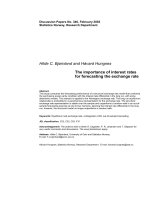
Figure 1: The Effect of the Zero Bound in a Severe Recession and Deflation
0
4
8
12
16
20
24
28
32
36
40
44
48

18.0

12.0
6.0
0.0
6.0
Output Gap
Quarter
with zero lower bound
without zero lower bound
0
4
8

12
16
20
24
28
32
36
40
44
48
15.0
10.0
5.0
0.0
5.0
Annual Inflation
Quarter
0
4
8
12
16
20
24
28
32
36
40
44
48


18.0

12.0
6.0
0.0
6.0
ShortTerm Nominal Interest Rate
Quarter
0
4
8
12
16
20
24
28
32
36
40
44
48
6.0
3.0
0.0
3.0
6.0
ExAnte LongTerm Real Interest Rate
Quarter
0

4
8
12
16
20
24
28
32
36
40
44
48
5.0
0.0
5.0
10.0
15.0
Real Effective Exchange Rate
Quarter
ECB • Working Paper No 218 • March 2003
18
Figure 1 compares the outcome of this sequence of contractionary and deflationary
shocks when the zero bound is imposed explicitly (solid line) to the case when the zero
bound is disregarded and the nominal interest rate is allowed to go negative (dashed-dotted
line). As indicated by the dashed-dotted line, the central bank would like to respond to
the onset of recession and disinflation by drastically lowering nominal interest rates. If
this were possible, that is, if interest rates were not constrained at zero, the long-term real
interest rate would decline by about 6% and the central bank would be able to contain the
output gap and deflation both around -8%. The reduction in nominal interest rates would
be accompanied by a 12% real depreciation of the currency.

However, once the zero lower bound is enforced, the recessionary and deflationary shocks
are shown to throw the Japanese economy into a liquidity trap. Nominal interest rates are
constrained at zero for almost a decade. Deflation leads to increases in the long-term real
interest rate up to 4%. As a result, Japan experiences a double-digit recession that lasts
substantially longer than in the absence of the zero bound. Rather than depreciating, the
currency temporarily appreciates in real terms. The economy only returns slowly to steady
state once the shocks subside.
Of course, the likelihood of such a sequence of severe shocks is extremely small. We
have chosen this scenario only to illustrate the potential impact of the zero bound as a
constraint on Japanese monetary policy. It is not meant to match the length and extent
of deflation and recession observed in Japan. While Japan has now experienced near-zero
short-term nominal interest rates and deflation for almost eight years, the inflation rate
measured in terms of the CPI or the GDP Deflator has not fallen below -2 percent. To
assess the likelihood of a severe recession and deflation scenario such as the one discussed
above, we now compute the distributions of output and inflation in the presence of the zero
bound by means of stochastic simulations.
ECB • Working Paper No 218 • March 2003
19
Figure 2: Frequency of Bind of the Zero Lower Bound on Nominal Interest Rates

1.0
1.5
2.0
2.5
3.0
3.5
4.0
4.5
5.0


10
0
10
20
30
40
50
Frequency of Bind (in Percent)
Equilibrium Nominal Interest Rate
3.3 The Importance of the Zero Bound in Japan
The likelihood that nominal interest rates are constrained at zero depends on a number
of key factors, in particular the size of the shocks to the economy, the propagation of
those shocks throughout the economy (i.e. the degree of persistence exhibited by important
endogenous variables), the level of the equilibrium nominal interest rate (i.e. the sum of the
policymaker’s inflation target and the equilibrium real interest rate) and the choice of the
policy rule. In the following we present results from stochastic simulations of our model with
the shocks drawn from the covariance matrix of historical shocks.
12
In these simulations we
consider alternative values of the equilibrium nominal interest rate, i
∗
= r
∗
+ π
∗
, varying
between 1% and 5%. Taylor’s rule is maintained throughout these simulations except if the
nominal interest rate is constrained at zero.

Figure 2 shows the frequency of zero nominal interest rates as a function of the level of
the equilibrium rate i
∗
. With an equilibrium nominal rate of 3%, the zero bound represents
a constraint for monetary policy for about 10% of the time. It becomes substantially more
12
The derivation of this covariance matrix and the nature of the stochastic simulations are discussed in
more detail in the appendix.
ECB • Working Paper No 218 • March 2003
20
important for lower equilibrium nominal rates and occurs almost 40% of the time with a
rate of 1%, which corresponds, for example, to an inflation target of 0% and an equilibrium
real rate of 1%.
Figure 3: Distortion of Stationary Distributions of Output and Annual Inflation
Output Annual Inflation

1.0
1.5
2.0
2.5
3.0
3.5
4.0
4.5
5.0


0.12
0.09
0.06

0.03
0.00
0.03
Bias of Mean
Equilibrium Nominal Interest Rate

1.0
1.5
2.0
2.5
3.0
3.5
4.0
4.5
5.0


0.03
0.00
0.03
0.06
0.09
0.12
Bias of Standard Deviation
Equilibrium Nominal Interest Rate

1.0
1.5
2.0
2.5

3.0
3.5
4.0
4.5
5.0


0.24

0.18

0.12

0.06
0.00
0.06
Bias of Mean
Equilibrium Nominal Interest Rate

1.0
1.5
2.0
2.5
3.0
3.5
4.0
4.5
5.0



0.06
0.00
0.06
0.12
0.18
0.24
Bias of Standard Deviation
Equilibrium Nominal Interest Rate
Whenever the zero bound is binding, nominal interest rates will be higher than pre-
scribed by Taylor’s rule. Similarly, the real interest rate will be higher and stabilization of
output and inflation will be less effective. Since there exists no similar constraint on the
upside an asymmetry will arise. The consequences of this asymmetry are apparent from
ECB • Working Paper No 218 • March 2003
21
Figure 3. As shown in the top left and top right panels, on average output will be some-
what below potential and inflation will be somewhat below target. Both panels display
this bias in the mean output gap and mean inflation rate as a function of the equilibrium
nominal interest rate. With an equilibrium nominal rate of 1% the downward bias in the
means is about 0.2% and 0.1% respectively. The lower-left and lower-right panels in Figure
3 indicate the upward bias in the standard deviation of output and inflation as a function
of the equilibrium nominal interest rate. For example, for an i
∗
of 1% the standard devia-
tion of the output gap increases from 1.51 to 1.59 percent, while the standard deviation of
inflation increases from 1.65 to 1.70 percent.
Figure 4: Stationary Distributions of the Output Gap and the Inflation Gap
6.0
3.0
0.0
3.0

6.0
Inflation Gap
Percentage Points
5.0
2.5
0.0
2.5
5.0
Output Gap
Percentage Points
i* = 1
i* = 3
Figure 4 illustrates how the stationary distributions of the output and inflation gaps
change with increased frequency of zero interest rates. Each of the two panels shows two
distributions, generated with an equilibrium nominal interest rate of 3% and 1% respec-
tively. In the latter case, the distribution becomes substantially more asymmetric. The
pronounced left tails of the distributions indicate an increased incidence of deep recessions
and deflationary periods. For example, for an i
∗
of 1% the probability of a recession of
at least -1.5 times the standard deviation of the output gap which would prevail if the
ECB • Working Paper No 218 • March 2003
22
zero bound were absent is 8.8 percent compared to 6.7 percent if the interest rate were
unconstrained.
As we discussed in the preceding subsection these deep recessions carry with them
the potential of a deflationary spiral, where the zero bound keeps the real interest rate
sufficiently high so that output stays below potential and re-enforces further deflation. This
points to a limitation inherent in linear models which rely on the real interest rate as
the sole channel for monetary policy. But it also brings into focus the extreme limiting

argument regarding the ineffectiveness of monetary policy in a liquidity trap. Orphanides
and Wieland (1998), which conducted such a stochastic simulation analysis for a model
of the U.S. economy, ensured global stability of the model by specifying a nonlinear fiscal
expansion rule that would boost aggregate demand in a severe deflation until deflation
returns to near zero levels. In this paper, we will instead follow Orphanides and Wieland
(2000) and introduce a direct effect of base money, the portfolio-balance effect, that will
remain active even when nominal interest rates are constrained at zero. This effect will
ensure global stability under all circumstances. With regard to the preceding simulation
results, we note that deflationary spirals did not yet arise for the variability of shocks and
the level of the nominal equilibrium rate considered so far.
As discussed above, the distortion of output and inflation distributions is driven by a
distortion of the real interest rate. The left-hand panels of Figure 5 report the upward bias
in the mean real rate and the downward bias in the variability of the real rate depending on
the level of the nominal equilibrium rate of interest. The downward bias in the variability of
the real rate accounts for the reduced effectiveness of stabilization policy. What is perhaps
more surprising, is the appreciation bias in the mean of the real exchange rate and the
downward bias in its variability as shown in the right-hand panels of Figure 5. This
reduction in the stabilizing function of the real exchange rate is consistent with what we
observed in the recession and deflation scenario discussed in the preceding subsection.
ECB • Working Paper No 218 • March 2003
23
Figure 5: Distortion of Stationary Distributions of the Determinants of Output
Ex-Ante Long-Term Real Interest Rate Real Effective Exchange Rate

1.0
1.5
2.0
2.5
3.0
3.5

4.0
4.5
5.0


0.08
0.00
0.08
0.16
0.24
0.32
Bias of Mean
Equilibrium Nominal Interest Rate

1.0
1.5
2.0
2.5
3.0
3.5
4.0
4.5
5.0


0.32

0.24

0.16


0.08
0.00
0.08
Bias of Standard Deviation
Equilibrium Nominal Interest Rate

1.0
1.5
2.0
2.5
3.0
3.5
4.0
4.5
5.0


0.40
0.30
0.20
0.10
0.00
0.10
Bias of Mean
Equilibrium Nominal Interest Rate

1.0
1.5
2.0

2.5
3.0
3.5
4.0
4.5
5.0


0.40
0.30
0.20
0.10
0.00
0.10
Bias of Standard Deviation
Equilibrium Nominal Interest Rate
4 Exploiting the Exchange Rate Channel of Monetary Policy
to Evade the Liquidity Trap
4.1 A Proposal by Orphanides and Wieland (2000)
Orphanides and Wieland (2000) (OW) recommend expanding the monetary base aggres-
sively during episodes of zero interest rates to exploit direct quantity effects such as a
portfolio-balance effect. The objective of this proposal is to stimulate aggregate demand
and fuel inflation by a depreciation of the currency that can be achieved by simply buying
ECB • Working Paper No 218 • March 2003
24
a large enough quantity of foreign exchange reserves with domestic currency. OW indicate
a concrete strategy for implementing this proposal within a small calibrated and largely
backward-looking model.
13
Following OW we use equation (1) to express the policy setting

implied by Taylor’s interest rate rule (equation (M-6)) in terms of the monetary base:
k
t
− k
∗
= −

κ
π
( π
(4)
t
− π
∗
)+κ
q
q
t

, (2)
where the response coefficients (κ
π
,κ
q
) correspond to Taylor’s coefficients of 1.5 and 0.5
given the normalization of θ = 1 used by OW and discussed in section 3.1.
Next, we allow the relative quantities of base money at home and abroad to have a direct
effect on the exchange rate in addition to the effect of interest rate differentials. Due to this
so-called portfolio-balance effect, the nominal exchange rate s
t

need not satisfy uncovered
interest parity (UIP) exactly:
14
s
(i,j)
t
=E
t

s
(i,j)
t+1

+0.25

i
(j)
t
− i
(i)
t

+ λ
b

b
(i)
t
− b
(j)

t
− s
(i,j)
t

. (3)
Here the superscripts (i, j) refer to the two respective countries. b
t
represents the log of
government debt including base money in the two countries. Rewriting UIP in real terms
and substituting in the monetary base as the relevant component of b
t
for our purposes, we
obtain an extended version of the expected real exchange rate differential originally defined
by equation (M-8) in Table 1:
e
(i,j)
t
=E
t

e
(i,j)
t+1

+0.25

i
(j)
t

− 4E
t

p
(j)
t+1
− p
(j)
t

− 0.25

i
(i)
t
− 4E
t

p
(i)
t+1
− p
(i)
t

(4)
+ λ
k

k

(i)
t
− k
(j)
t
− e
(i,j)
t

.
Given λ
k
> 0, the monetary base still has an effect on aggregate demand via the real
exchange rate even when the interest rate channel is turned off because of the zero bound.
13
As a short-cut they specify a reduced-form relationship between the real exchange rate, real interest
rate differentials and the differential Marshallian k instead of the uncovered interest parity condition.
14
This specification from Dornbusch (1980, 1987) is also considered by McCallum (2000) and Svensson
(2001).