WORKING PAPER SERIES NO. 546 / NOVEMBER 2005: THE NATURAL REAL INTEREST RATE AND THE OUTPUT GAP IN THE EURO AREA A JOINT ESTIMATION doc

WORKING PAPER SERIES
NO. 546 / NOVEMBER 2005
THE NATURAL REAL
INTEREST RATE AND
THE OUTPUT GAP
IN THE EURO AREA
A JOINT ESTIMATION
by Julien Garnier
and Bjørn-Roger Wilhelmsen
In 2005 all ECB
publications
will feature
a motif taken
from the
€50 banknote.
WORKING PAPER SERIES
NO. 546 / NOVEMBER 2005
This paper can be downloaded without charge from
or from the Social Science Research Network
electronic library at />1 Work on the project began while Julien Garnier was doing an internship and Bjørn-Roger Wilhelmsen was on secondment at the
European Central Bank. All views expressed in the paper are only those of the authors and are not necessarily those of the European
Central Bank (ECB) or the institutions to which the authors are affiliated.We are grateful to Siem Jan Koopman for very helpful
suggestions and comments.We also thank P. Cour-Thimann,V. Curdia, F. Drudi, S. McCaw, D. Rodriguez-Palenzuela, R. Pilegaard, H. Pill,
L. Stracca,T. Laubach, J. C.Williams and the participants of the ECB workshop on natural interest rates on Februar 19th 2004.
2 European University Institute and University of Parix X-Nanterre.; e-mail:
3 Central Bank of Norway, Economics Department; e-mai:
THE NATURAL REAL
INTEREST RATE AND
THE OUTPUT GAP
IN THE EURO AREA
A JOINT ESTIMATION

1
by Julien Garnier
2
and Bjørn-Roger Wilhelmsen
3
© European Central Bank, 2005
Address
Kaiserstrasse 29
60311 Frankfurt am Main, Germany
Postal address
Postfach 16 03 19
60066 Frankfurt am Main, Germany
Telephone
+49 69 1344 0
Internet

Fax
+49 69 1344 6000
Telex
411 144 ecb d
All rights reserved.
Any reproduction, publication and
reprint in the form of a different
publication, whether printed or
produced electronically, in whole or in
part, is permitted only with the explicit
written authorisation of the ECB or the
author(s).
The views expressed in this paper do not
necessarily reflect those of the European

Central Bank.
The statement of purpose for the ECB
Working Paper Series is available from
the ECB website, .
ISSN 1561-0810 (print)
ISSN 1725-2806 (online)
3
ECB
Working Paper Series No. 546
November 2005
CONTENTS
Abstract 4
Non-technical summary 5
1 Introduction 6
2 The data 7
3 A review of the recent empirical literature:
short vs long-run perspectives 8
4 Estimating the natural rate of interest 9
4.1 The model 9
4.2 Model estimation 11
4.3 Results 12
5 Statistical properties of the real interest gap
in the euro area 18
6 Conclusion 19
References 20
Appendices 22
European Central Bank working paper series 28
4
ECB
Working Paper Series No. 546

November 2005
Abstract


The notion of a natural real rate of interest, due to Wicksell (1936), is widely used in current
central bank research. The idea is that there exists a level at which the real interest rate would
be compatible with output being at its potential and stationary inflation. This paper applies the
method recently suggested by Laubach and Williams to jointly estimate the natural real
interest rate and the output gap in the euro area over the past 40 years. Our results suggest that
the natural rate of interest has declined gradually over the past 40 years. They also indicate
that monetary policy in the euro area was on average stimulative during the 1960s and the
1970s, while it contributed to dampen the output gap and inflation in the 1980s and the 1990s.

Key words: Real interest rate gap, output gap, Kalman filter, euro area

JEL Classification Numbers: C32, E43, E52, O40

5
ECB
Working Paper Series No. 546
November 2005
Non-technical summary

The notion of a natural rate of interest knows a revival of interest in current monetary
policy research. From a theoretical point of view, the natural real rate of interest is a central
concept in the literature because it provides policymakers with a benchmark for monetary policy:
Interest rates above the natural rate are expected to lower inflation, whereas rates below the
natural rate are expected to raise inflation. In practice, however, the natural real rate is
unobservable and has to be estimated.
According to recent contributions to the literature, the concept of the natural real interest

rate and the concept of potential output should be consistent, so that given the definition of
potential output it will be clear how to define the natural real interest rate. The two equilibrium-
variables are expected to change together over time with shocks and should therefore not be
estimated independently. In line with this argument we estimate the natural real rate of interest
and potential output simultaneously using data for the euro area, Germany and the US.
The modelling framework consists of a small macroeconomic model encompassing an IS
curve and a Phillips curve that connects inflation, the output gap and the real interest rate gap,
defined as the difference between the real short term interest rate and estimates of the natural real
interest rate. In addition, the natural real interest rate is linked to the potential growth rate of the
economy. This produces an estimate of the natural real interest rate that varies over time in
harmony with lower-frequency evolutions in the real economy. We use relatively long datasets,
starting in the early 1960s.
Our results suggest that the natural real rate of interest in the euro area and Germany has
declined gradually over the past 40 years, while the natural real interest rate in the US has been
more stable around its long term average. The natural rate of interest in the euro area was, on
average, higher than the actual rate in the 1960s and 1970s, while it was lower compared to the
actual rate most of the time in the 1980s and 1990s. In other words, monetary policy was
stimulative during the 1960s and 1970s, while it was on average tight in the 1980s and 1990s.
Regarding the output gap, the length of the business cycle’s booms and busts are in line
with the consensus view in the business cycle literature. However, the estimated output gap is
influenced by the real interest rate gap, which implies that its average level is positive in periods
of loose monetary policy (1960s and the 1970s) and negative in periods of tight monetary policy
(1980s and 1990s). Indeed, the coefficient of correlation between the real interest rate gap and the
output gap is strongly negative for the euro area. Moreover, we argue that the real interest rate
gap may contain valuable information about future inflation in the euro area. However, it should
be borne in mind that estimates of the natural real interest rate are imprecise.
1Introduction
In the long run, economists assume that nominal in terest rates will tend to ward some equi-
librium, or ”natural”, real rate of interest plus an adjustment for expected long-run inflation.
The natural rate of in tere st is a cen tral concept in the mon eta ry policy literature since it

provides policyma kers with a benchmark for monetary policy. In theory, it is important for
evaluating the policy stance sin ce rates a bo ve (belo w ) the n atura l rate a re expected to lo wer
(raise) inflation.
From an empirica l point of view, the "natural" r eal rate of in ter est is unob servab le.
The estimation of th e natural r eal interest rate is not str aightforward an d is associated
with a very high degree of u n certainty. In practice, therefore, policymak ers cannot rely
exclusively on the real interest rate gap, defined as the difference between the real short term
in terest rate and estimates of the natural real in terest, as an indicator of the monetary policy
stance. Rather, a c omprehensive approac h using a wi de set of information is re quired. This
notwithstanding, central bank economists have increasingly devoted attention to developing
estimation strategies for the natural real in terest rate. The methods used range from as
simple as calculating the average actual real interest rate over a long period to building
dynamic stochastic general equilibrium (DSG E) models with nominal rigidities.
A recent contribution s to the literature on how to empirically a pp roa ch the c o ncep t
of the natural rate is a paper by Laubach and W illiams (2003; henceforth LW)
1
with an
application to data for the United States. They suggest to estimate the natural real interest
rate and potential output gro w th simultaneously, using a small-scale macroeconom ic model
and K alm an filtering tec h n iques. In this m odel, the natural real interest rate is rela ted t o
the poten tial gro w th rate of the economy. Thus, the estimate of the natural real in terest
rate is time-var ying and r elated to lon g-term d evelopments i n th e real c har acteristics of the
economy, consisten t with econo m ic theory. This m eth od has become popular since it strikes
a c ompromise bet ween th e theoretically coherent DS G E approac h and ad-hoc s tatistical
approaches, as e mphasized by Larsen and M cKeo w n (2002).
In this paper we employ the technique of LW for the e uro area. The present work differs
from ot hers in that we use a relatively l ong ( synthetic) dataset starting in t he early 1960s.
Besides, we estimate the natu ral real interest rate in G erman y and the U S for comparison.
Such comparison is interesting because, prior to 1999, monetary policies in Europe wer e con-
siderably influenced b y the Bundesban k policy. At the same time, the US is often considered

as a useful pro xy for global influences that affect monetary policy worldwide. T h ird, w e
apply sim p le statistical tests to inv estig ate the leading indicator properties of the baseline
estimate of the euro area real interest rate gap on inflation and ec onomic activity.
Thepaperisstructuredasfollows.Insectiontwowetakealookatthedataforthereal
in terest rate from 1960. Sections three reviews the recent empirical literature and discusses
the n atu ral rate concept in t he context of differen t horizons. Section fou r presen ts the
1
Some papers have already used this framework on European data, including Sevillano and Simon (2004)
for Germany, Larsen and McKeow n (2002) for the United Kingdom and Crespo-Cuaresma et al (2003) and
Mésonnier and Renne (2004) for the euro area.
6
ECB
Working Paper Series No. 546
November 2005
modeling approach and displa ys the estimation results. Section five briefly discusses the
leading indicator properties of the estimated real rate gap. Section six concludes.
2 The data
In this section we tak e a closer look at th e data used in this study. The data co vers a to tal
of 161 q ua rterly observations from 1963q1 to 2004q1 for the eur o area an d Germa ny an d 162
quarterly observations from 1961q1 to 2002q4 for the U S . The dataset con sists of sho rt-ter m
in terest rates, inflation and Gross Domestic Products for the three econom ies
2
. The compu-
tation of real interest rates is subject to several pra ctical and c on cep tual difficulties . Ide a lly,
an estimate of the real in terest rate should be obtained by substracting ex an te inflation
expectations from nominal interest rates. Ho wev er, the lac k of good data for inflation ex-
pectations forces us to take a more straightforward approach. In this paper, th e real interest
rates are calculated fro m the th ree-m onth money m arket rates and annual consumer price
inflation rates
3

. While we believe that the problem with using current inflation as a proxy
for inflation expectations is less severe when assessing developments over longer horizons,
the deviations may be stronger in periods with unanticipa ted inflation, notably in the 19 70s.
It should be borne in mind th at monetary policy regim es differed significan t ly ov er time
and a cross co untries. Moreov er, in m any euro a rea co untries, specifically in the 1960s and
early 1970s, other instruments than in terest rates were important in the conduct of mon etary
policy. In p ar ticular, capital controls prevailed in many e uro a rea countries. Furtherm ore,
inflation, econom ic gr owth and interest rates were very volatile in some e uro area coun tries.
Finally, the euro area real interest rate has been significantly influenced by other factors
than monetary policy, suc h a s tensions within the Exchange Rate M ec hanism (ERM) at the
turn of the 1990s (Cour-Thimann et al, 2004).
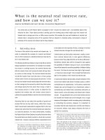
The euro area real interest rate fell dramatically in the 1970s, when o verheated economies
and rising oil prices pushed up inflation at a leve l that could not be offset by the nominal real
interest ra tes (See Fig ur e 1 ). Fo llowing the trough in the mid-197 0s, a s European m on etar y
authorities gradually put more emphasis on disinflationary policies, th e real in te rest rate
increased slo wly over a period o f more than 15 years. After peaking in the early 1990s, the
real rate declined gradually ag ain, influenced by the monetary authorities’ ac h ievemen t of
more favourable inflation developemen ts.
Similar to the euro area a gg regate, the real in terest ra te in the U nited Sta tes was also
lo wer than average in the 1970s and higher thanitsaverageinthe1980s. However,the
persistence in the data seems less pronounced, as in dica ted by the quick rise in the r eal r ate
at the turn of the 1980s. In Germ any the real interest rate has been more stable around
its long-term average, reflecting the achievment o f lower a n d more stable inflation ov er the
whole sample.
2
We are grateful to the ECB for providing the data for Germany and the euro area, and Thomas Laubach
and John C. Williams for providing the US data.
3
For the euro area, national levels for interest rates and consumer prices have been aggregated prior to
1999 using GDP and consumer spending weights respectively at PPP exchange rates, see ECB (2003).

7
ECB
Working Paper Series No. 546
November 2005
1965 1970 1975 1980 1985 1990 1995 2000 2005
0
5
Germany
1965 1970 1975 1980 1985 1990 1995 2000 2005
0
5
10
US
1965 1970 1975 1980 1985 1990 1995 2000 2005
0
5
10
Euro area
Figure 1: Real interest rates
3 A review of the recen t em pirical literature: short vs long-run
perspectives
The c oncept of a natural rate of interest was first introduced by Knut Wicksell in the late
19
th
century (1898, with 1936 translation ). Today the concept kno w s a revival of in terest
following Wood ford’s seminal book, Interest a n d Prices. Accord ing to the recent literature,
fluctua tions in the real interest rate may be decom posed in to t wo different components: a
natural real r ate and a real r ate gap (Woodford, 2003; Neiss a nd Nelson, 2003; Cour-Th ima nn
et al, 2004). The natural rea l rate is related to stru ctur al factors an d is the real in terest rate
that in theory w ould prevail under perfectly flexible prices. This is comm o nly referred to

as th e "Wicksellian" definition of the natura l ra te of in terest. The real in terest rate gap is
related to the business cycle an d reflects the existence of nominal rigidities in the economy.
The a vailab le estimates of historical dev elop m ents in the euro area natural real interest
rate differ considerably from one author to the other. We briefly address these d ifferences
belo w and classify estimates o f th e natural r eal rate, taking as cirterium the time horizon a t
which they s hould be interpreted.
Some papers find that most of the flu ctu ations in the real in t erest rate should be at-
tributed to fluctua tions in the real interest rate gap rather than the natural real interest
rate. This group of papers, which includes Giammarioli and Valla (2003), Mésonnier and
Renne (200 4), Ne iss and Nelson (20 03 ), Sevilliano and Sim o n (200 4) and LW, a ssociate the
fluctua tions in the natural real interest rate with the evolution of real fundamen ta ls such as
determ inants of trend GDP growth and p r eferences. These va r iables are typically stable in
the short to medium term, but ma y d isplay some variation in the longer run. Consequently,
8
ECB
Working Paper Series No. 546
November 2005
the natural real interest rate is also relativ ely stable in the short run, and the natural rate in
these papers sh ould be consider ed in a ”long-run” perspective . It refers i nd eed to the lev el
expected to p reva il in, say, the next fiv e to ten y ears, after any business c ycle ”booms” and
”busts ” underw ay ha ve played out. Note ho wever that the estimated natural real rate of
Méson nie r and R en ne (2004) i s mu ch m ore vo latile that tha t of LW or Sev illian o and S im on
(2004).
On the contrary, ot her p apers conclude that fluctuations in the natural real interest rate
explain m ost of t he variatio n in t h e real interest rate (B asdeva nt et al, 2004; Cu aresma et
al, 2004; Cour-Thimann et al, 2004; Larsen and McKeow n, 2002). The papers consistent
with this view typ ically make use of the Kalman filter or other filtering t echniques to split
the actual r eal r ate into a tren d ( the n atu ral real rate) and a cyclical com ponen t (the real
rate gap ). How ever, the models they use d o not necessarily co ntain judgem ents about the
determinants of the natural rate. Rather, the approac h they tak e is closer to a pure statistical

measur e. C on sequently, variations in the natural rate are more pronou nced , because the
natural rate tends to follow more closely the medium term fluctuation s in the actual real
rate. The in terp retation of the natural real interest rate in this context is therefore likely
to be m ore rel eva nt in a ”shorter” tim e perspective i n that it refers to a neutral moneta ry
policy stance in a situation where the economy has not necessarily settled at its long-run
levels.
4 Estim ating the natural rate o f in tere st
This paper tak es a ”long-run ” time-perspectiv e and uses economic theory as a benc hm ar k for
determ ining the d evelopments in the na tural real interest rate. As r eca lled b y LW, standard
gro wth models im ply that the natural real in terest rate v aries over time in response to shifts
in preferences a nd the trend gro wth rate of output, t hem selves unobservable variables.
4.1 The model
The empirical frame work suggested by LW is to run the Kalman filter on a system of equ a-
tions to j o intly estim ate the na tura l real interest rate, potentia l output g rowth and th e
output gap. They propose a model of a neo-keynesian inspiration, that join tly c haracterises
the behaviour of inflation and t he output gap t hrough m odified IS and P h illips c urves.
Neo-keynesian models a re not so much i nterested in th e levels of variables co m posing these
curves, but rath er the deviations fr om equilibrium values. The main equation s o f the m odel
are given by:
a
y
(L)˜y
t
= a
r
(L)˜r
t
+ ε
1,t
(1)

b
π
(L)π
t
= b
y
(L)˜y
t
+ ε
2,t
(2)
where ˜r
t
is the real in terest rate gap , ˜y
t
represents the output gap defined as the difference
bet ween the (log) GD P y
t
and (log) poten tial outpu t y
∗
t
suc h tha t
˜y
t
=100(y
t
− y
∗
t
) (3)

9
ECB
Working Paper Series No. 546
November 2005
π
t
is consumer price inflation, ε
1,t
and ε
2,t
are white noise errors, and a
y
,a
r
,b
π
and b
y
are
polynomials in the lag operator L such that a
y
(L)=−
P
n
i=0
a
y,i
L
i
, with a

y,0
= −1.
The laws of motion o f u nobservable poten tial ou tput an d i ts tren d g rowth rate are spec-
ified as the following:
y
∗
t
= y
∗
t−1
+ g
t−1
+ ε
4,t
(4)
g
t
= g
t−1
+ ε
5,t
(5)
where ε
4,t
and ε
5,t
are white noise errors.
The economic theory i m posed by LW is represented by the fo llowing relation ship for the
natural real in terest rate:
r

∗
t
= cg
t
+ z
t
(6)
where g
t
is the unobservable trend grow th rate of th e economy, whic h is linked to the natural
real interest rate r
∗
t
with the parameter c, capturing the r ela tive r isk aversion. z
t
represent
other possible determinants of the natural rate of in terest, suc h as households time pref-
erences, variation in public saving and uncertatinty about interest rates. z
t
is assumed t o
follow a stoc h astic pr ocess determined by:
z
t
= αz
t−1
+ ε
3,t
(7)
In LW , z
t

, is either a stationary AR process or a random walk. The measure of t he random
determ inants of the n atu ra l real interest rate, z
t
,is ob v iou sly associated with a considerable
degree of uncertainty. We face here a techn ical problem in that r
∗
t
is an un ob served variable,
itself com posed of two unobserved components. This d ifficult y has already been poin ted out
b y Méson nier & Renne (2004). In most of the specifications that we ha ve tried, the results
were highly sen sitive to initial cond itions a nd were often not rea son able. This is especially th e
case wh en z
t
follows a rando m walk. In de ed , wh ile th e first elemen t g
t
is explicitly linked to
the output t hrough (3) and (4), z
t
is only defined through (7), w hich makes it more sensitiv e
to small var iations in the initial specifications of the m odel. To o vercome this problem, we
only co nsid er th e c ase where z
t
follows a stationary AR process, and we restrict its varia nce
σ
2
3
through a signal-to-noise ratio, λ
z
. Weelaboratefurtheronthispointinthenextsection.
In addtion, w e claim that the po ssible eleme nts composing z

t
should be sta tion ar y, th er eby
making a random walk spe cification useless.
Equa tion (4), (5), (6) and (7) constitute the state (transitory) equations of our state-
space model, and the IS curv e (1) and the Phillips cu rve (2) constitute the observation
equations (see Harv ey (1989)). On this system, the Kalman filter is ru n t w ice: first i n
order to iden tify param e ters b y m aximum likelihood, and second in order to estimate the
unobserv ed componen ts r
∗
t
, y
∗
t
, g
t
and z
t
. Th e m odel can be w ritten und er its state-space
form (see appendix A):
y
t
= Zα
t
+Bx
t
+Gε
t
(8)
α
t+1

= Tα
t
+Hε
t
(9)
10
ECB
Working Paper Series No. 546
November 2005
4.2 Model esti mation
Theprocedurefollowsdifferen t steps, in line w ith the recom m endations of LW. The first one
is to get a p rior estimation of th e output gap. Fo r this p urpose, we use a segmented lin ear
trend with breaks in 1973 and 1993, a s a proxy for poten tial output. initial output
gap is then used to estimate the coefficients of the simplified system b y OLS : a
y
(L)˜y
t
=
a
r
(r
t−1
+r
t−2
)+ε
1,t
(for the IS equation) and b
π
(L)π
t

= b
y
(L)˜y
t
+ε
2,t
(for the Phillips curve).
This prov ides us with adequate starting values for the maxim u m likelihood estimation of the
coefficien ts.
In a second step, w e consider a simplified system similar t o the pr eviou s one, except that
we estimate th e coefficients by m aximum lik elihood and we use the Kalman filter . P otential
output y
∗
t
is treated as an unobserve d componen t:
a
y
(L)˜y
t
= a
r
(r
t−1
+ r
t−2
)+ε
1,t
b
π
(L)π

t
= b
y
(L)˜y
t
+ ε
2,t
y
∗
t
= y
∗
t−1
+¯g + ε
4,t
where ˜y
t
is the output gap, r
t
is the real interest rate, and ¯g is a constant.
The third step is dedicated to finding a median un biased estimate of the variance of
potential o utput growth, σ
2
5
.
4
For t h is purpose, we use the estimate of y
∗
t
from the previous

step in o rder t o run th e median u nbiased technique of Stock & Watson (1998). The procedure
works as follo ws: 1) Regress for every date t the potential output growth
5
on a constant and
adummywithabreakattimet. 2) Comp ute the t-ratios corresponding to the c oefficients
of the dumm ies. 3) Comp ute the Exponen tial Wald (EW ) statistic
6
. Itaddsthet-ratios
obtained at ever y date. 4) Compare the values obtained with that of Stock & Watson’s
table that maps these statistics to the value of median unbiased signal-to-noise ratios λ.
Once w e ha ve found the adequate ratio λ
g
,
7
it sufficestoplugitintoσ
5
= λ
g
σ
4
in order to
get the adequa te m ea sure o f poten tial ou tput. We prov ide belo w (ap pendix B) a sen sitivity
analysis of the model by taking different percentiles of the distribu tion of λ
g
’s, compute d
from 10 .000 draws of the monte carlo simulation procedure used by LW.
As exposed above, the variance of z
t
is set according to the signal-to-noise ratio λ
z

=
a
r
√
2
σ
3
σ
1
.
8
We use once a gain th e median unbiased estim ator. A lthough this technique is only
needed in theory w hen z is non-stationary, it should provide an adequate w ay to estimate
4
The reason for using this approach is that the bulk of the distribution of the parameters that control for
the variance is often very close to zero. Consequently, the maximum likelihood estimates of these parameters
are often statistically insignificant, and are far below the median of the distribution. This would imply for
instance that g
t
would be constant.
5
i.e. ∆y
∗
t
,wherey
∗
t
is computed as in step 2 above.
6
such that EW =ln(

1
T
P
T
i=1
exp(s
2
i
/2)) where s
i
is the t-ratio corresponding to a break at time i.
7
We keep here the same notation as LW.
8
√
2 comes from the assumption that the output gap in equation (1) is determined by a moving average
of the real interest gap of order 2. That is, ˜y is in fluenced by z
t−1
and z
t−2
through a single coefficient, a
r
.
See the following section.
11
ECB
Working Paper Series No. 546
November 2005
The
λ

z
, even with stationary p rocesses. For this purpose, we compute the monte carlo procedure
of LW to get a distribution for λ
z
. We use the median of this distribution as our baseline
value. That is, we take λ
z
=0.064. The 5th percen t ile is 0.046 and the 95th 0.076.
The final s tep estimates the whole system (1) to (7) by m ax imum l ikelihood
9
,withthe
two ratios λ
g
and λ
z
imposed. We pr oceed in two step s: First, we estimate the whole system
and sto re th e IS curve output lag coefficients. Second, we re-estimate th e system with these
coefficien ts fixed. Fo r some reason, the estimated output gap with this procedure is much
more in line with the existing literature than in the case of a simple, one-step estima tion.
In order to identify the model, w e hav e to restrict some par am eters. For instance, the
variance parameters were restricted to be strictly positive. This is comm on practice in the
literature. We also use some constraints that are specific to t he model. For example, w e
impose a
g
= c.a
r
≤ 0, since there should be a mechanical negativ e relation between the
growth rate g
t
of potential output y

∗
t
and the output gap ˜y
t
= y
t
− y
∗
t
. T his in t urn implies
that th e coefficien t c is positive , wh ich is a lso intuitive because th is coefficien t i s s upposed
to cap tu re consum e rs’ relativ e risk aver sio n . Following LW, we also take a simple mo v in g
average of the first and second lags of ˜r
t
. This co m es d own to im posing the sam e c oefficien t
on these two elements. We impose in a d dition that th e resulting coefficien t a
r
is les s than or
equal to zero, since the real rate gap should be countercyclical.
In practice, we follow LW and assum e th a t the polynomials a
y
(L) and a
r
(L) in e q uation
(1) are of ord er 2, while b
y
(L) in (2) is simply of o rd er 1. b
π
(L) is of order 3, but instead of
taking the second and third lags of π

t
, i.e. π
t−2
and π
t−3
, we take moving averages of the last
three quarters of the first y ear and the whole previous year, such that : π
0
t−2
=
P
4
i=2
π
t−i
and π
0
t−3
=
P
8
i=5
π
t−i
.
4.3 Results
This section reports and discusses the estimation results. Table 1 sho ws param eter estimates
for the euro area, Germany and the US. The natural rate estimates, and the uncertaint y
surroundin g the estima tes, are fairly similar to those reported b y LW o n U S data.
AsregardstheIScurve,thesumofthecoefficients of the autoregressive componen ts of

the output gap, a
y
(L), lies between 0.83 and 0 .93 for all countries. The effect of a change in
therealinterestrategapontheoutputgap,a
r
, seems to be so m ew ha t weeker in the euro
area than in the US and German y. The effectofachangeintheoutputgaponinflation,
on th e o th er hand, seems t o be slightly stronger i n the euro a rea c ompared t o t h e US and
Germany. The null h ypothesis that the coefficients of the inflation terms, b
π
(L),sumtoone
in the Phillips curve is not rejected by th e data .
9
The BFGS procedure for numerical optimization is u sed for this purpose.
12
ECB
Working Paper Series No. 546
November 2005
1965 1970 1975 1980 1985 1990 1995 2000 2005
-2
0
2
4
6
8
Figure 2: Natural real interest rate r
∗
t
estimate and ±2 s.d.
Table 1 : Par am eter estim ates, baseline m odel

Eur o Are a Germany US
63q1-04q1 63q1-04q1 61q1-02q2
Variances
λ
g
0.081 0.081 0
λ
z
0.064* 0.064* 0.064*
σ
IS
0.005 0.008 0.006
σ
Phillips
0.396 0.473 0.776
σ
y∗
0.003 0.004 0.004
σ
g
= λ
g
.σ
y∗
2.43×10
−4
3.24×10
−4
0
IS curve

a
y1
0.70 (1.88) 0.47 (1.23) 1.63 (6.63)
a
y2
0.14 (1.81) 0.36 (1.23) -0.70 (6.75)
a
r
-0.056 (2.42) -0.172 (1.47) -0.18 (1.96)
c 0.880 0.653 1.179
Phillips curve
b
π1
1.18 (6.25) 1.07 (4.65) 0.77 (3.04)
b
π2
-0.28 (5.34) -0.14 (4.00) 0.13 (2.60)
b
π3
=1− (b
π1
+ b
π2
) 0.1* 0.07* 0.09*
b
y
0.051 (9.31) 0.041 (7.73) 0.103 ( 18.01)
t statistics in parentheses
*: imposed coefficient
13

ECB
Working Paper Series No. 546
November 2005
Regard ing the estim ate of th e natural real inter est rate in the e uro area, F igure 2 r eveals
a very high uncer taint y aro un d th e e stim ate o f the level of r
∗
t
. How ev er, as indicated by the
sensitivity analysis in the appendices, w e argue that this is essentially due to the uncertaint y
surrounding the coefficien t c. If w e impose a con straint on the possible r ange of values this
coefficien t can take, the range of estimates of the level of the natural real interest rate di-
minishes. For almost all signal-to-noise ratios in the mod el (having fixed the c coefficient to
its baseline estim ate), the estimated natural real interest rate seem s to have been higher in
the 1 960s and early 1970s than i n the 1990s and 2000s. M oreover, t he natural real i nterest
rate seems to have been higher in 1990, when the reunifica tion of E ast and West Germany
took pla ce, co m p ared to the period after the Stage Three o f Monetary and Economic Union
(EM U). Furthermore, the estimated na tural real interest rate w a s also lower in 20 04 co m -
pared to the start of Stage Three of the EMU in 1999. Finally, our baseline estimate (the
bold li ne in F igure 2) su ggests that th e natural r eal interest rate has declined from around
4% in the 1960s to less than 2% in 2004.
In the model, the d ecline in the natural real inter est rate in the eu r o area is largely due
to a fall in the estimated trend grow th rate of the economy (see Figure 3)
10
.Giventhe
imp recision of the Kalm a n filter estimate of trend GDP growth, we com p ar e our estima te
with estimates based on the Hodric k -P rescott filter for which we use t wo different values of
the smoothing parameter lambda (1600 and 50 000). The larger v alue of lam bda mak es the
resulting trend smoother (less high-fr equen cy noise), while the smaller lam bda mea ns the
trend follo w s the d ata more closely. Figure 3 sh ows that the volatility o f the Kalma n filtered
trend grow th is, on a verage, fairly similar t o the Hod rick-Prescott filter estimate when using

a relatively large va lu e o f the l a mbda. For all estimates, the trend grow th o f th e economy
has declined over the sam ple.
Figure 4 s hows our baseline estim ate o f the euro area output gap (com pared with esti-
mates from HP filter and B a xter and King’s bandpass filter), whereas figure 5 a nd 6 s how
dataforconsumerpriceinfla tion and o ur baseline estimate of the real interest ra te gap r espec-
tiv e ly. The estimated ou tput ga p is consistent with the com m on ly held v iew t ha t m oneta ry
policy w as loose in the 1 9 70s, contributing to a positiv e output gap and a persisten tly high
level of inflation for most of the decade. M oreover, in th e early 1980s, a s m on etary policy
authorities in man y countries pur sued tigh t monetary policy orien ted towards disinflation
11
,
the output gap turned negative. Except f or a small positive output gap in the beginning of
the 1990s, the output gap remained negative until the start of Stage T h ree of EMU .
In ter estin gly, F igu re 5 show s that inflation began to decline almost imm ed iate ly after the
estimated real interest rate gap turned positiv e in the 1980s. A s noted by LW , univaria te
filtering would, by th eir nature of two-sided weighted averages, lead to estimates of t he
natural real in terest rates and potential outp ut that are, on aver age, relativ ely close to
10
Cour-Thimann et al (2004) provide very plausible arguments for the view that increases in government
debt in the 1980s and higher exchange rate risk premia in the early 1990s might have put upward pressure on
the natural real rate in the euro area. These arguments imply that our estimate of the natural real interest
rate in this period is somewhat low.
11
See for instance Taylor (1992) for a description of the disinflation policy in the US.
14
ECB
Working Paper Series No. 546
November 2005
1965 1970 1975 1980 1985 1990 1995 2000 2005
1.5

2.0
2.5
3.0
3.5
4.0
4.5
5.0
1.5
2.0
2.5
3.0
3.5
4.0
4.5
5.0
g
t
(baseline model)
Δ
4
y
HP(50000)

Δ
4
y
HP(1600)


Figure 3: Estimated potential output grow th g

t
and fourth differences of HP-filtered output.
the a ctu al r eal interest r ate and actual output du ring the 1970s, even thou gh inflation was
increasing. For this reason, the Kalman filter generally provides more reasonable r esu lts of
the real interest rate gap and the outpu t gap than un ivariate time-series me thods.
Figure 7 com pares the ba seline estim ates of the natura l real in terest ra tes for the euro
area, Germany a nd the US. Eviden tly, w hile the estimated natural real i nterest rate in the
euro area an d G erm any has declined ov er the sam ple, the natural real interest rate in the
US h a s been m o re stab le around its long term average. The estimates also indicate that the
lev el of the natural real in terest r ate is lower in the euro area, and in particular in Germany,
than in the US .
It is i mportant to stress that all estimates of the natural real inter est rate are very
imprecise and that caveats are associated with all estimation methods. Regarding the pitfalls
with the approa ch taken in this paper, the estimation results are very sensitive to initial
specifications of the m odel and the selection o f starting values for th e parameters. A second
aspect concerns the measurement of time-varia tion in preferences (see equation 3 ). Third,
non-textbook factors that may contribute to time variation in t h e na tur al r ate are treated
arbitrarily. W ithin the empirical framework of this paper, variable z
t
is supposed to represent
all other factors than trend output growth to explaining the dev elopments in the natural real
in terest rate. Argu ab ly, the preciseness o f this m ea sure is very doubtful, w hich c o uld make
the estimates difficult to interpret.
15
ECB
Working Paper Series No. 546
November 2005
1965
1970
1975

1980
1985
1990
1995
2000
2005
-
2.5
0.0
2.5
5.0
Baseline output gap,
~
y
t

Baxter & King cycle, y
BK

HP output gap, y−y
HP


1965
1970
1975
1980
1985
1990
1995

2000
2005
-2.5
0.0
2.5
5.0
1965
1970
1975
1980
1985
1990
1995
2000
2005
-2.5
0.0
2.5
5.0
Figure 4: Baseline estim ate of outpu t gap
1965
1970
1975
1980
1985
1990
1995
2000
2005
-5.0

-2.5
0.0
2.5
5.0
7.5
10.0
12.5
15.0
-5.0
-2.5
0.0
2.5
5.0
7.5
10.0
12.5
real interest rate gap
Inflation
Figure 5: Natural real interest rate gap ˜r
t
(= r
t
− r
∗
t
) and inflation rate, euro area.
16
ECB
Working Paper Series No. 546
November 2005

1965 1970 1975 1980 1985 1990 1995 2000 2005
-5.0
-2.5
0.0
2.5
5.0
~
r
t
euro area
~
r
t
Germany
Figure 6: Natu ral real in ter est rate gap ˜r
t
(= r
t
− r
∗
t
),euroareaandGermany.
1965
1970
1975
1980
1985
1990
1995
2000

2005
2
3
4
2
3
4
Euro area
r* average r*
1965
1970
1975
1980
1985
1990
1995
2000
2005
1
2
3
1
2
3
Germany
1965
1970
1975
1980
1985

1990
1995
2000
3.0
3.5
4.0
3.0
3.5
4.0
US
Figure 7: Baseline estim ates of r
∗
t
for the euro area, Germany and the US
17
ECB
Working Paper Series No. 546
November 2005
5 Statistical pro perties of the real in te re st gap in the euro area
We now e xam in e some statistical properties of the euro area m odel, focusing on simple
statistics that d escribe the relationship between the real interest rate gap and in flation.
Table 2 and 3 report standard deviations a n d correlations of selected variables used in this
analysis, namely log output y
t
, log potential output y
∗
t
, the output gap ˜y
t
, the actual and

the natural real rate an d the real rate gap (r
t
,r
∗
t
and ˜r
t
) and i nflation π
t
. A notable feature
of the reported statistics is that the correlation between the actual real in terest rate and
the real interest rate gap are high an d their standard deviations are roughly identical. In
other w or ds, the variation in the real inte rest rate is not prim arily related to variation in
the natural real interest ra te. This is consisten t with the results in Giamm ario li and Valla
(2003) for t he euro area, Neiss and Nelson ( 2 003) for the U K and LW for the US, but stands
against the results of Cour-Thimann (2004) for the euro area.
Table 2 :
Standard deviations, e uro area
y
t
0.35
y
∗
t
0.30
˜y
t
1.72
π
t

3.50
r
t
2.55
r
∗
t
0.80
˜r
t
2.93
Table 3 : Correlation coefficients, euro area
k =0 k =1 k =2 k =3 k =4
Corr(r
t
, ˜r
t−k
) 0.98
Corr(π
t
, ˜r
t−k
) -0.47 -0.48 -0.50 -0.53 -0.55
Corr(˜y
tt
, ˜r
t−k
) -0.5 5 -0.57 -0.59 -0.6 0 -0.62
In ter estin gly, the correlation bet ween inflation and the real rate gap is strongly ne gative
at all lags. This indicates that the developments in euro area inflation since 1960 are, in

part,relatedtotheevolutionoftherealinterestrategap. Inlinewiththishypothesiswe
find that the real rate gap is also strongly and negatively correlated with the output gap.
Next, w e investigate the leading indica tor properties of the real in terest rate gap for inflation.
Follow in g Ne iss and N elson (20 03 ), we estimate:
π
t
= a + b
1
π
t−1
+ b
2
(r
t−k
− r
∗
t−k
)+ε
t
18
ECB
Working Paper Series No. 546
November 2005
where annual inflation π
t
is regressed on p ast inflat ion and lagged values of the real
in terest rate gap. The regression on the 1962:1 - 2003:1 samp le is summ a rised in table 4
(numbers in parantheses are standard errors). The results indicate that lagging the rea l
interest rate gap 3 to 5 quarters yields statistically significant parame ter estimates when
added to an autoregression for inflation. The long lags seem consisten t with the common

view that monetary policy affects inflation after a significan t delay. This simple exercise
suggests tha t th e estim a ted r eal interest rate gap may contain valuable info rm a tion a bout
futur e inflation.
Table 4 : Parameter estim ates, euro area
k =1 k =2 k =3 k =4 k =5
a 0.08 0.10 0.13 0.15 0.18
b
1
0.98 0.98 0.97 0.97 0.97
b
2
−0.02
(−1.53)
−0.03
(−1.97)
−0.04
(−2.85)
−0.05
(−3.07)
−0.06
(−3.70)
R
2
0.98 0.98 0.98 0.98 0.98
6Conclusion
This paper estimates the natural real interest rate for the euro area, considering the currency
union as a single en tity over the pe r iod 1963 to 2004, and for Germany and the US. Follo w in g
closely the m ethodology suggested by Laubach an d Williams (2003), we apply th e Kalman
filt er to a small scale macroeconomic model, which encompasse s a Phillips curv e and an IS
curve. This allo w s us to estimate the n atu ra l real interest r ate, po tential output and t rend

growth rate o f the th ree economies simultaneously. Overall, the results are quite c omparable
with the origina l results of Lau ba ch and William s (2003 ) using U S d ata .
Accord ing to o u r ba seline estim a te for th e e uro a rea, the fluctuations in the n atural real
interest rate have been relativ ely low since 1963. The natural rate has declined gradually
ov e r the past 40 yea rs, from an estimat e of around 4% in the 1960s to slightly less than
2% in 2004. The real interest rate gap is relatively persisten t o ver l on ger periods, with low
short-term fluctuations. Moreov er, the real interest rate gap in dicated that m onetary policy
was on average sti mulativ e in the 1960s and 1970s, while it contributed to dam pen economic
activit y and inflation in the 1980s a n d 1990s.
Regard ing the output gap, the length of the business cycle’s booms and busts are in
line with the consensus view i n the business cycle literature. However, this model produces
an ou tput gap that is influenced by the real in terest rate gap. Its average level is negative
in periods of tight mo neta ry policy and positiv e in periods of monetary laxism. T h is is
interesting since it might be taken as a n indicator of the degree at which the central bank
policy influences the real econom y. In the 1970s when inflation become high. the real in terest
rate gap w as negative an d the output gap was positive, on a verage. L ik e wise, in the 1980s
and 1990s, when inflatio n fell to lower levels, the real interest rate w as positive and the
output gap w as on negative, o n average.
Simple empirical t ests also suggest that the estimated real interest rate gap is n eg atively
19
ECB
Working Paper Series No. 546
November 2005
correlatedwiththeoutputgapandinflation. Fu rtherm ore, the tests show that t he real rate
gap m ay contain valuable i nform ation about f uture inflation i n the euro area. The general
ca veats associated with interpretin g estimates of the natural real in terest rate, whic h are
highly u n certa in, also app lies for this pa per.
References
[1] Bar ro, R.J . and Sa la-i-Martin, X. (1995): "Econo m ic G rowth.": McGraw-Hill.
[2] Basd eva nt, O.N . Björksten and O. Ka rag edikli (2004): "Estimating a time varying

neutral real interest rate for New Zealand ", R eserve B a nk of New Zealand Discussion
P aper, DP2004/01
[3] Blanc hard, O. and S. Fischer (1989): "Lectures on Macroeconomics.": Cambridge, M A :
MIT -p ress.
[4] Co ur-Thiman n, Philip pin e, Rasmus Pilegaa rd a n d Liv io Str acc a (200 4): "The o utpu t
gap and the real in terest rate gap in the euro area, 1960-2003", paper presented at the
Bank of Canada workshop on Neutral Interest Rates, 9-10 September 2004 (a vailable
on Bank of Canada’s website).
[5] Cu aresm a, J.C., Gn an, E . and D. Ritzberger-Grun enw ald (2004): "Searc hin g for a
natural rate of in terest: a euro area perspective" , Em pirica, vol 31, p. 185 - 204
[6] De L ong an d J. Brad fo rd (1997 ): "America’s Peacetime Inflation: the 1970s ", in C.D.
Romer a nd D.H. Romer ( eds.), Reducing Inflation : Motivation and Strategy. Chicago:
Universit y of Chicago P ress. 247-276
[7] Ford, Robert and Douglas Laxton (1999), "World Public Debt and R eal In terest R ates",
Oxford Review of Economic Po licy, Vol. 15 No.2.
[8] G riam m a rioli, N icola a nd Natac h a Valla ( 20 03), "T h e Natural Rate o f Interest in th e
Euro area", ECB Working P aper No. 233
[9] Harvey, A n drew C. (1989): "Forecasting, structural time series model and the Kalman
filter", Cambridge University P ress, Ca mbridge.
[10] Koopman S .J., Shepha rd N . and Doornik J.A. (1998), "Statistical algorithm s for
models in state sp ace using S sfPac k 2.2", Econometrics Journal, 1, 1-55 and
h ttp://www.ssfpack.com/
[11] Larsen, Jens D. J. and Jac k M cK eown (2002), "The information conten t of empirical
measures of real in terest rate and output gaps for the United Kingdom", BIS papers
No 19
[12] Laub ach, Th om as and J oh n C. W illia m s (2003), "M ea surin g the Natu ra l Rate of Inter-
est", Review of Econom ics and Statistics, vol 85(4), p. 1063-1070
[13] Lev in, A., V. Wieland an d J.C .Williams (20 03 ). "Ro bu stness o f Sim ple M o neta ry Policy
Rules under Model Uncertain t y " in Jo hn B. Taylor, ed. Monetary Policy Rules, Chicago.
University of Chicago P ress. pp, 263-299

[14] M aravall, A. (1995) “U no bser ved Components in Economic T ime Series”, in
M.H .Pesaran and M.R.W ick ens (eds.), Hand book of app lied econometrics. Vo lum e 1.
Macroeconom ics. Han dbooks in Economics, Blackw ell, Oxfo rd an d M ald en, 12-72.
[15] Mésonnier, J S, and J P. Renne (2004) “A Time-Varying Natural Rate of Interest for
20
ECB
Working Paper Series No. 546
November 2005
theeuroarea”,WorkingpaperNo115,BanquedeFrance.
[16] Neiss, K. and Nelson, E ( 2003): "The real rate gap as an Inflation Indicator ", Macro-
economic Dyn amics, 7, pp. 239 - 262.
[17] Nelson, E. (2004): "The Great Inflation of t he Seventies: W ha t really Happened?", Fed
working paper, J anuar 2004
[18] Nelson, E. and K. Nik olov (2002): "Monetary P olicy and Stagflation in the U.K. " Bank
of England Working paper No. 155, May
[19] N elson, E. and K. Niko lov (2003): "U.K. Inflation in t h e 1970s a nd 1980s: the R ole of
Outp ut Gap Mism ea sur em ent", Journal of Econom ics a ns Business, Vo l. 55 (4), 353-370.
[20] Proietti, T. ( 2001) “Unobserved Componen ts Models for Measuring Output G aps, Ca-
pacity Utilisation and Core Inflatio n”, mimeo, notes prepared for the course ‘Unob-
served C o m ponen ts Models a nd their A p plication s in Macroeconomics’, European Cen-
tral Bank, 11 and 12 June 2001.
[21] Sevillano, J. M. M. and M. M. Simon (2004): “An empirical approxim ation of the nat-
ural rate of interest an d poten tial gro w th ”, Working paper No 0416, Banco de Esp ana.
[22] Stock J. a n d M.Watson (1998), "Median un b iased estimation of coefficient varia nce
in a time-vary ing parameter model", Journal of the American Statistical Association,
March, 93, p.349-358.
[23] Stokey, N and S. Rebelo ( 1995 ): "Growth Effects of F lat-R ate Taxes. " Jo urnal of
Politic al Economy.Vol.103,No.3.
[24] Taylor, John B . (1992): "The great i nflation, the great di sinflation a nd policies for
future price stabilit y. " I n A. Blun d ell-Wignall (ed), Inflation, Disinflation and M onetary

Policy. Sydney. Am b assador press. 9-34.
[25] W icksell, K. (1898) "In terest and prices", London, Macm illan, 1936. Tra n sla tion of 1898
edition
[26] W illiam s, J.C . (2003 ) "T he natu ral rate of interest", FRBS F E con omic letter 2003-32
[27] Woodford, M. (2003): "Interest and prices: foundations of a theory of monetary policy",
Princeton U niversit y P ress.
21
ECB
Working Paper Series No. 546
November 2005
A ppend ices
AState-spaceform
The system to be estimated, eq (1), (2), (4), (5) and (7), has to be put into the general
state-space form:
α
t+1
= Tα
t
+Hε
t
(10)
y
t
= Zα
t
+Bx
t
+Gε
t
(11)

where Z, B, G, T and H are matrices of coefficien ts
12
. (10) is the so-called measu rem ent
equation and (11) the state equation. y
t
is a vector of d ependent variables, corr esponding
to y
t
and π
t
in our model, α
t
is a vector c orresponding to the u nobserv ed compo nen ts,
here y
∗
t
,g
t
and z
t
. r
∗
t
is suppressed from th e model because it can be fully reco vered from
g
t
and z
t
, prov ided we obtain c. x
t

is a vector of determ inistic variables. ε
t
∼ NID(0, I)
and α
0
∼ N(a, P). N o te that th e representation of (12) is particular in that the vector of
parameters B is treated as a vecto r of unobserved variables. This is a feature of the library
Ssfpack for Ox that w e use in this paper.
The system c an be rewritten
⎛
⎝
α
t+1
B
y
t
⎞
⎠
=
⎛
⎝
T 0
0 I
Zx
t
⎞
⎠
µ
α
t

B
¶
+
⎛
⎝
u
t
0
v
t
⎞
⎠
(12)
= Φ
µ
α
t
B
¶
+ u
t
, u
t
∼ NID(0, u
t
u
0
t
)
where α

0
t
=
¡
y
∗
t
y
∗
t−1
··· y
∗
t−n
g
t
g
t−1
z
t
z
t−1
¢
, B
0
=
¡
Ca
x
··· a
rx

b
x
··· b
sx
¢
,whereC equals 0
or ρ, depending on the specificiation of z
t
(see eq. 7).
T =
⎛
⎜
⎜
⎜
⎜
⎜
⎜
⎜
⎜
⎜
⎜
⎜
⎝
10··· 010 0 0
1 ··· 00 0
.
.
.
.
.

.
.
.
.
.
.
.
.
.
.
.
.
.
0 ··· 10 0
10
.
.
. 10
10
0 ··· 010
⎞
⎟
⎟
⎟
⎟
⎟
⎟
⎟
⎟
⎟

⎟
⎟
⎠
Z =
µ
1 −a
y1
··· −a
yn
0 −c.a
r
0 −a
r
0 −b
y1
··· 00··· ··· 0
¶
x
t
=
µ
0 x
1t
··· x
rt
0 ··· 0
00··· 0 x
0
1t
··· x

0
st
¶
12
We assume here that they are constant since this is the specification used in our model, but they could
just as well be defined as time-varying parameters.
22
ECB
Working Paper Series No. 546
November 2005
and u
0
t
=
¡
ε
4,t
0 ··· 0 ε
5,t
0 ε
3,t
0 ··· ··· 0 ε
1,t
ε
2,t
¢
.
Y
t
=

µ
Y
1
Y
2
¶
=
µ
y
t
− a
y1
y
t−1
− − a
yn
y
t−n
− a
r
r
t−1
π
t
− b
π1
π
t−1
− − b
πp

π
t−p
− b
y
y
t−1
¶
The specification of the v ecto r of dependen t variables allo w s us to impose constraints on
the coefficients on som e of the variables (e.g. y
t
and y
∗
t
). The other exogenous variables,
namely the dummies x
t
, are e stim a ted as in a classical regression model, i.e. are t reated as
unobserved variables, upon whic h no con straint can be imposed.
B Se nsitivity analysis
B.1 Shorter sample
1965 1970 1975 1980 1985 1990 1995 2000 2005
0
1
2
3
4
5
0
1
2

3
4
5
λ
g
restricted
c restricted
full sample, baseline
unrestricted
λ
g
and c restricted

Figure 8: Shorter sample. r
∗
t
estimates 1973Q2-2004Q 2
23
ECB
Working Paper Series No. 546
November 2005
B.2 Sensitivit y to si gnal-to-noise ratios: unrestricted c
1965
1970
1975
1980
1985
1990
1995
2000

2005
-3
-2
-1
0
1
2
3
4
-3
-2
-1
0
1
2
3
4
Sensitivity of r
*
to λ
g
(λ
z
= 0.064, baseline value)
λ
g
= 0.081 (baseline)
λ
g
= 0.12 (95th percentile)

λ
g
= 0.013 (5th percentile)

Figure 9: The natu ral real interest rate. Sensivity to signal to noise ratios with unrestr icted c.
1965
1970
1975
1980
1985
1990
1995
2000
2005
-17.5
-15.0
-12.5
-10.0
-7.5
-5.0
-2.5
0.0
2.5
5.0
-17.5
-15.0
-12.5
-10.0
-7.5
-5.0

-2.5
0.0
2.5
5.0
Sensitivity of output gap to λ
g
(λ
z
= 0.064, baseline value)
λ
g
= 0.081 (baseline)
λ
g
= 0.12 (95th percentile)
λ
g
= 0.013 (5th percentile)

Figure 10: Th e output gap. Sensivity to signal to noise ratios with unrestricted c.
24
ECB
Working Paper Series No. 546
November 2005