An Audit Environment for Outsourcing of Frequent Itemset Mining potx

An Audit Environment for Outsourcing
of Frequent Itemset Mining
W. K. Wong
The University of
Hong Kong

David W. Cheung
The University of
Hong Kong

Edward Hung
The Hong Kong
Polytechnic University

Ben Kao
The University of
Hong Kong

Nikos Mamoulis
The University of
Hong Kong

ABSTRACT
Finding frequent itemsets is the most costly task in associa-
tion rule mining. Outsourcing this task to a service provider
brings several benefits to the data owner such as cost re-
lief and a less commitment to storage and computational
resources. Mining results, however, can be corrupted if the
service provider (i) is honest but makes mistakes in the min-
ing process, or (ii) is lazy and reduces costly computation,
returning incomplete results, or (iii) is malicious and con-

taminates the mining results. We address the integrity issue
in the outsourcing process, i.e., how the data owner verifies
the correctness of the mining results. For this purpose, we
propose and develop an audit environment, which consists of
a database transformation method and a result verification
method. The main component of our audit environment is
an artificial itemset planting (AIP) technique. We provide
a theoretical foundation on our technique by proving its ap-
propriateness and showing probabilistic guarantees about
the correctness of the verification process. Through analyt-
ical and experimental studies, we show that our technique
is both effective and efficient.
1. INTRODUCTION
Association rule mining discovers correlated itemsets that
occur frequently in a transactional database. A variety of
efficient algorithms for mining association rules have been
proposed [1, 2, 4]. The problem can be divided into two
subproblems: (i) computing the set of frequent itemsets,
and (ii) computing the set of association rules based on the
mined frequent itemsets. While the latter problem (rule
generation) is computationally inexpensive, the problem of
mining frequent itemsets has an exponential time complex-
ity and is thus very costly. This motivates businesses to
outsource the task of mining frequent itemsets to service
Permission to copy without fee all or part of this material is granted provided
that the copies are not made or distributed for direct commercial advantage,
the VLDB copyright notice and the title of the publication and its date appear,
and notice is given that copying is by permission of the Very Large Data
Base Endowment. To copy otherwise, or to republish, to post on servers
or to redistribute to lists, requires a fee and/or special permission from the

publisher, ACM.
VLDB ‘09, August 24-28, 2009, Lyon, France
Copyright 2009 VLDB Endowment, ACM 000-0-00000-000-0/00/00.
providers. With outsourcing, a data owner exports its data
to a service provider, who returns the set of frequent item-
sets together with their support counts. Apart from cost
relief, outsourcing also brings a number of benefits. For ex-
ample, if data is transient and only a statistical summary (as
captured by frequent itemsets and association rules) is de-
sired, the data owner can ship its data to a service provider
without archiving them locally.
1
As another benefit, trans-
actional data collected at different sources (such as those
generated at different stores of a chain supermarket) can be
consolidated and processed at the service provider. The ser-
vice provider can find the frequent itemsets that are local
to each individual source, or the global frequent itemsets for
the whole organization. The cost of transferring transac-
tions among the sources and performing the global mining
in a distributed manner can be saved. Finally, with out-
sourcing, the data owner does not need to maintain an IT
team for the data mining task.
For outsourcing to be practical, the issues of security and
integrity have to be addressed satisfactorily. Regarding se-
curity, the data owner has to ensure that neither the content
of its data nor the mining result is disclosed to the service
provider. This security problem has been addressed in [16],
in which an encryption scheme was devised to protect data
content and mining results. In this paper we focus on the

integrity problem, that is, how the data owner can ensure
the correctness of the mining results. The results of this
paper, combined with the techniques we proposed in [16]
for enforcing security, constitute a complete solution to the
outsourcing problem.
The first step towards solving the integrity problem is to
understand the behavior of a (potentially malicious) service
provider that can undermine the integrity of the mining re-
sults. A service provider may return inaccurate results if (i)
it is honest but sloppy, e.g., there are bugs in its mining pro-
grams; (ii) it is lazy and tries to reduce costly computation,
e.g., it mines only a small portion of the dataset; (iii) it is
malicious and purposely returns wrong results, e.g., a busi-
1
This is an alternative approach to applying a data mining
algorithm for streaming data [9]. The advantage is that with
outsourcing the data owner receives the complete and exact
set of frequent itemsets from the service provider, while ap-
plying a streaming data mining method only computes an
approximate solution to the problem.
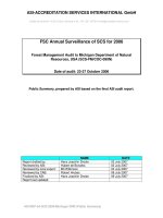
T
Data owner
T T
FI
Transformations
Service provider
FI
Audit Environment
Frequent
Itemsets

FI
Verifications
auxiliary
data
^
^
U
R
Figure 1: The architecture of the scheme
ness competitor has paid the service provider for providing
incorrect results so as to affect the business decisions of the
data owner. The concept of result integrity should thus be
defined on two criteria:
• Correctness: All returned frequent itemsets are actu-
ally frequent and their returned support counts are
correct.
• Completeness: All actual frequent itemsets are included
in the result.
A straightforward attempt to solving the integrity prob-
lem is to verify the mining results against the database —
we scan the database once to count the support of each fre-
quent itemset reported in the result. These support counts
are then compared against those returned by the service
provider. Though simple, this approach has a number of
shortcomings. First, it verifies the correctness criterion but
not the completeness criterion. It fails to detect frequent
itemsets that are missing in the result. Second, it is some-
what costly. The verification requires scanning the complete
database once and counting the supports of a (potentially)
large set of itemsets. Third, it requires the original database

to be available. If the content of the database is continu-
ously updated, an image dump has to be taken and archived
(for later verification). This adds to the cost of the mining
exercise, particularly when the database is large. It is thus
not suitable for applications such as those related to data
streams.
Our approach to solve the integrity problem is to con-
struct an audit environment. Essentially, an audit environ-
ment consists of (i) a set of transformation methods that
transform a database T to another database U, based on
which the service provider will mine and return a mining
result R; (ii) a set of verification methods that take R as
an input and return a deduction of whether R is correct
and complete; (iii) auxiliary data that assist the verifica-
tion methods. An interesting property of our approach is
that the audit environment forms a standalone system. It is
self-contained in the sense that the verification process can
be done entirely by using only the auxiliary data that are
included in the environment. In other words, the original
database need not be accessed during verification. Figure 1
shows the architecture of our scheme.
The core component of our audit environment is a tech-
nique of database transformation and verification called ar-
tificial itemset planting (AIP). AIP provides probabilistic
guarantees that incorrect or incomplete mining results re-
turned by the service provider will be identified by the owner
with a controllably high confidence. To give the intuition be-
hind AIP, we briefly describe it here (more details will be
given in Section 4.1). Given a set of itemsets


F I, AIP gen-
erates a (small) artificial database
ˆ
T such that all itemsets
in

F I are guaranteed to be frequent and their exact support
counts are known. Also, the original database T and
ˆ
T con-
tain disjoint sets of items. T is then transformed to U by
merging transactions in T with those in
ˆ
T (i.e., a transaction
in
ˆ
T is appended to the end of some transaction in T ). The
idea is that when the service provider mines U , the set

F I
(and the associated support counts) will be part of the min-
ing result R. Since the service provider cannot distinguish
itemsets of T from those of
ˆ
T , if the result R is incorrect
or incomplete, there are high chances that the returned

F I
is also incorrect or incomplete. So, by verifying


F I, we are
able to obtain a probabilistic guarantee on whether the re-
sult integrity is enforced. Essentially,

F I serves as a fragile
watermark of the mining result — perturbation of the result
will very likely destroy the integrity of

F I.
Our Contributions. The contributions of this work in-
clude: (i) a formal definition of a model of malicious actions
that a service provider might perform to undermine result
integrity; (ii) a novel artificial itemset planting (AIP) tech-
nique for constructing an audit environment; (iii) a theoret-
ical study on the cost and effectiveness of AIP technique;
and (iv) an empirical study to evaluate the performance of
the proposed methods.
The rest of the paper is organized as follows. Section 2
reviews related work. Section 3 defines our model of mali-
cious service providers and an audit environment. Section 4
describes the AIP technique for constructing an audit envi-
ronment. We propose efficient algorithms for implementing
AIP and give an analytical study on the algorithms. Sec-
tion 5 empirically evaluates the performance of AIP, both
in terms of its effectiveness in detecting malicious actions
performed by a service provider and the efficiency of our
algorithms. Finally, Section 6 concludes the paper.
2. RELATED WORK
The problem of outsourcing the task of data mining with
accurate result was first introduced in our previous work

[16]. There, we address the security issues in outsourcing
association rule mining. An item mapping and transaction
transformation approach was proposed to encrypt a transac-
tional database and to decrypt the mined association rules
returned from a service provider. This paper focuses on the
integrity issues and thus complements the study in [16]. A
data owner can apply both techniques to protect sensitive
information and at the same time verify the result returned
from the service provider. To the best of our knowledge,
integrity issues in outsourcing data mining have not been
studied before.
The most similar model to outsourcing data mining is
the outsourced database model [5]. A data owner exports
its database to a service provider who processes queries by
the owner and reports results. A number of papers have
been published on the integrity problem of the outsourced
database model [7, 12, 8, 15, 17, 11]. For example, in [7, 12,
8], Merkle hash trees are built on both the owner side and the
service provider side to achieve authentication of query re-
sults. As another example, in [11], each record in a database
is digitally signed. The proposed signature scheme has an
interesting property that missing tuples in query results can
be detected. In the above examples, queries are limited to
those that look for sets of tuples as answers (such as point
and range queries). Aggregate queries are not supported.
In [15], an alternative strategy, called challenge token, was
proposed. The scheme allows general queries (point, range,
aggregate) to be verified; challenge tokens (queries whose
answers are known) are submitted to the service provider
together with regular queries. In addition to the query

answers, the service provider finds and returns the tokens,
which are then used as proof of integrity. The scheme, how-
ever, can only guard against “sloppy” and “lazy” providers,
who do not intentionally return incorrect or incomplete re-
sults. Malicious providers may selectively answer challenge
tokens correctly but provide wrong answers for other queries.
They can thus work around the scheme. In [17], fake tuples
are injected into a database. By tracking the fake tuples,
query results are probabilistically verified. The advantage
of this scheme is that it works conveniently on off-the-shelf
database systems. The method is thus unintrusive (unlike,
e.g., the Merkle-hash-tree-based methods). The drawback
of the fake-tuple scheme is that it does not support aggre-
gate queries. In the outsourced data mining model, query
results are composed of statistical aggregations (e.g., item-
set counts in association rule mining, centroid computation
in clustering). The above technique is thus not applicable.
The integrity problem in outsourced frequent itemset mining
has not been addressed.
A major difference between the outsourced database model
and the outsourced mining model is that for the former,
a service provider is expected to answer numerous (small)
queries on the same database, while for the latter, one or
only a few mining exercises are performed for each instance
of the database. A larger amount of resources, such as stor-
age and preparation cost can be invested for the outsourced
database model, since the cost can be amortized over a large
number of owner queries. On the other hand, an outsourced
mining model should avoid high preparation cost, as it is
not expected to pay-off.

In the brief description of our artificial itemset planting
(AIP) technique (Section 1), we mentioned about generating
an artificial database
ˆ
T so that its (known) set of frequent
itemsets

F I can be used to verify the mining results. The
generation of the database
ˆ
T is a core part of AIP. Given
a set of frequent itemsets and the corresponding support
counts, the problem of generating a database that satisfies
the support constraints is proved to be an NP-hard prob-
lem [10]. In [3], an iterative approach that uses a greedy
heuristic is proposed to generate such a database. As we
have argued, the preparation cost of the outsourced mining
model should be small, the cost of the heuristic algorithm
put forward in [3] is still too high to be practical (e.g., the al-
gorithm requires multiple database scans). There are other
database generation algorithms previously proposed in the
literature, e.g., [13, 14]. Since many of the properties of the
generated databases (such as database size and the set of
frequent itemsets) cannot be precisely controlled, they are
not suitable for AIP. In this paper we propose a method
for efficiently generating an artificial database
ˆ
T for AIP.
Our database generation method does not contradict the
NP-hardness result proved in [10] because the set of fre-

quent itemsets

F I and the associated support counts are
not rigidly fixed. Instead, the constraints are dynamically
adjusted so that an efficient method for generating
ˆ
T is pos-
sible. Details about this database generation approach will
be discussed in Section 4.1.
3. MODEL
In this section we formally define the integrity problem in
outsourcing frequent itemset mining. We define notation,
state the properties of an audit environment, define the set
of malicious actions that a service provider might perform to
alter the mining results, and formulate the concept of “ma-
licious service provider gain” which captures the incentive
and penalty to a service provider for his malicious actions.
Let I be a set of items. A transaction t
i
is a subset of I.
A transaction t
i
contains an itemset x if and only if x ⊆ t
i
.
Given a database T that contains a number of transactions,
the support count of an itemset x is the number of transac-
tions in T that contain the itemset x. Let σ be a function
such that σ(x) gives the support count for any itemset x ⊆ I.
Given a support threshold s%, an itemset x is frequent if and

only if σ(x) ≥ |T | × s%, where |T | is the number of trans-
actions in T . The objective of frequent itemset mining is to
find all frequent itemsets and their support counts in T with
respect to a given support threshold.
3.1 Malicious Actions
Assume a party p
owner
owns a set of transactions T. An-
other party (service provider) p
miner
helps p
owner
to com-
pute the set of frequent itemsets L in T. The service provider
p
miner
is not trusted and it is possible that p
miner
performs
malicious actions and purposely modifies the mining results.
Let R = (L, σ) be the true result of mining (i.e., L is the
complete set of frequent itemsets and σ(x) gives the correct
support count for any x ∈ L). Let R

= (L

, σ

) be the re-
sult returned by p

miner
. R

may not equal R and p
miner
may
have performed a series of the following malicious actions:
Insertion. p
miner
includes an infrequent itemset in the
returned set of frequent itemset claiming that the itemset is
frequent. More specifically, p
miner
picks an itemset y /∈ L,
sets L

= L

{y}, and sets σ

(y) = r where r is an artificially
generated value that is greater than the support threshold.
σ

(x) = σ(x) for all x ∈ L.
Deletion. p
miner
excludes a frequent itemset from the
returned result. p
miner

picks an itemset y ∈ L and sets
L

= L − {y}. σ

(x) = σ(x) for all x ∈ L

.
Replacement. p
miner
returns a modified (incorrect) sup-
port count of a frequent itemset. p
miner
picks an itemset
y ∈ L, sets L

= L, and sets σ

(y) = r = σ(y) where r is an
artificially generated value that is greater than the support
threshold. σ

(x) = σ(x) for all x ∈ L

− {y}.
Every possible returned result given by the miner can be
simulated by a series of the above malicious actions. Inser-
tions and modifications contaminate the correctness of the
result while deletions affect the completeness of the result. If
it can be proved that the miner has not performed any of the

three malicious actions, the returned result will be both cor-
rect and complete. We remark that a malicious miner can be
easily caught if it performs the malicious actions randomly
since the returned set L

may not satisfy the monotonic-
ity property [1] (which states that any subset of a frequent
itemset must be frequent). For example, let I = {A, B, C}.
Suppose p
miner
computes L = {A, B, AB}. If p
miner
in-
serts AC to this result, the returned result to the owner is
L

= {A, B, AB, AC}. Note that L

does not satisfy the
monotonicity property (C is a subset of AC, however, AC
is frequent and C is infrequent). Similarly, if p
miner
deletes
B, but not AB, there will be an integrity violation due to
monotonicity. This observation leads us to the definition of
a valid return.
Definition 1. (Valid Return) A returned result R

=
(L


, σ

) is valid if ∀x ∈ L

, ∀y ⊂ x, y = ∅ ⇒ y ∈ L

and
σ

(y) ≥ σ

(x).
A smart but malicious miner should always give a valid
return, since violation of integrity in invalid returns can eas-
ily be detected. For example, if p
miner
decides to insert an
itemset x ∈ L to L

, he should also insert all the subsets of
x that are not in L. In the following discussion, we assume
that R

is always valid.
3.2 Expected Gain
When a malicious service provider performs a malicious
action, the mining result is contaminated and he is rewarded,
for example, from a business competitor of p
owner

. The
more malicious actions are performed, the more rewards are
earned. On the other hand, if a malicious action is detected,
the service provider not only loses the reward he would be
paid for performing the mining task, but should also com-
pensate p
owner
for returning incorrect results. In addition, if
the service provider is caught changing the results, he loses
its reputation in the industry, which is a big penalty. The
aim of the malicious service provider is to perturb the min-
ing result as much as possible without being noticed. We
model p
miner
’s gain and loss of perturbing mining results by
a measure called expected gain (EG).
Definition 2. (Expected Gain) Let R = (L, σ) be the
true result and R

= (L

, σ

) be the returned result. Let n
be the minimum number of malicious actions taken to ob-
tain R

from R and A
1
, A

2
, , A
n
be the corresponding
n malicious actions. Let φ be a scoring function such that
φ(A
i
) returns the score gained by performing A
i
. Let ρ be
the penalty the miner suffers if any of its malicious actions
is detected by p
owner
. Let p be the probability of such a
detection. The expected gain (EG) is given by, EG(R

) =
(1 − p)

n
i=1
φ(A
i
) − pρ.
Note that EG(R) = 0 if the miner returns the true result
R. The objective of a malicious miner is to find an R

such
that EG(R


) is maximized. If EG(R

) < 0 for all R

= R,
p
miner
should be forced to return the true result R, as he
will suffer a certain penalty for doing otherwise. The goal
of our audit environment is to transform the data prior to
outsourcing in order to force the service provider to return
the correct result.
3.3 Audit Environment
An audit environment consists of a set of transformation
methods, a set of verification methods, and auxiliary data
for verification. An audit environment is self-contained such
that the verification process can be carried out without ac-
cessing the original database. Moreover, it should satisfy
the following properties:
• Its preparation cost should be low. The resources put
in this process should be much less than the resources
required by the mining process.
• The audit environment should not induce a large over-
head to the service provider. In particular, mining the
transformed database U should not cost much more
than mining the original database T .
• The audit environment should be robust. In particu-
lar, the expected gain of a malicious miner should be
controllably small or even negative.
4. PREPARING THE AUDIT ENVIRONMENT

In this section we discuss how an audit environment can
be prepared efficiently. We first prove a theorem that allows
us to detect malicious insertions and deletions by examin-
ing the positive and negative borders of L

. We then discuss
a straightforward method for detecting malicious replace-
ments. We point out the drawbacks of the straightforward
method and propose our novel technique AIP. We start by
defining the terms negative border and positive border.
Definition 3. (Negative Border) Given an item domain
I, let S be a set of frequent itemsets that satisfy the mono-
tonicity property. The negative border of S, denoted by
B
−
(S), is the set of all minimal infrequent itemsets w.r.t.
to S, i.e., B
−
(S) = {x | x ⊆ I and x /∈ S and ∀y ⊂ x
where y = ∅, y ∈ S}.
Definition 4. (Positive Border) Given a set of frequent
itemsets S that satisfies the monotonicity property, the posi-
tive border of S, denoted by B
+
(S), is the set of all maximal
frequent itemsets w.r.t. to S, i.e., B
+
(S) = {x | x ∈ S and
∀y ⊃ x, y ∈ S}.
For example, if I = {A, B, C, D}, S = {A, B, C, AB, BC},

then B
−
(S) = {D, AC} and B
+
(S) = {AB, BC}.
Given a result R

= (L

, σ

) returned by p
miner
, we need
to verify that no malicious insertions, deletions, or replace-
ments have been applied. The following theorem shows that
insertions and deletions can be detected by examining the
borders of L

.
Theorem 1. Suppose p
miner
returns a valid return R

=
(L

, σ

) to p

owner
. No insertions are performed to the actual
set L if and only if all itemsets in B
+
(L

) are frequent in
p
owner
’s database and no deletions are performed if and only
if all itemsets in B
−
(L

) are infrequent in p
owner
’s database.
Proof. Insertion-if. We prove the transposition of the
statement. If the miner has inserted an itemset x, then x ∈
L

and x ∈ L. Since R

is a valid return, there must exist an
itemset y ∈ B
+
(L

) such that x ⊆ y. By the monotonicity
property, x ∈ L ⇒ y ∈ L. Hence, there exists y in the

positive border that is not frequent.
Insertion-only if. If no insertions are performed, the miner
must have only performed deletions and/or replacements.
So, L

⊆ L. Since B
+
(L

) ⊆ L

, all itemsets in B
+
(L

) are
frequent.
Deletion-if. We prove the transposition of the statement.
If the miner has deleted an itemset x, then x ∈ L and x ∈
L

. Since R

is a valid return, there must exist an itemset
y ∈ B
−
(L

) such that y ⊆ x. By the monotonicity property,
x ∈ L ⇒ y ∈ L. Hence, there exists y in the negative border

that is frequent.
Deletion-only if. If no deletions are performed, the miner
would have only performed insertions and/or replacements.
So, L ⊆ L

. Since B
−
(L

)

L

= ∅, we have B
−
(L

)

L =
∅. So, all itemsets in B
−
(L

) are infrequent.
From Theorem 1, we know that it is necessary that all sup-
port counts of itemsets in the borders B
−
(L


) and B
+
(L

)
are verified. Also, to detect replacement, we need to ver-
ify support counts of itemsets in L

. Therefore, an ideal
audit environment should include all the support counts of
itemsets in L


B
+
(L

)

B
−
(L

) = L


B
−
(L


) for verifi-
cation.
As we have argued, it is desirable that an audit environ-
ment be prepared as the database is exported to a miner.
The audit environment should also be self-contained so that
subsequent verification does not require accesses to the orig-
inal database (which might have already been updated or
unavailable during verification). Therefore, preparing such
an audit environment with support counts of all the item-
sets in L


B
−
(L

) is impractical because the set L

is not
known when the environment is being prepared. Also, find-
ing all these supports is equivalent to mining the database,
which defeats the purpose of outsourcing.
One possible approach to reduce verification cost is sam-
pling. For example, we select a set of itemsets Z and count
their supports. An audit environment includes all these
counts. Given a result R

= (L

, σ


), we verify the support
counts of itemsets in Z

(L


B
−
(L

)), effectively examin-
ing only a sample of L


B
−
(L

). A major problem with
the simple sampling strategy is that the universe of itemsets
is very large and thus most of the elements in Z may not be
in L


B
−
(L

). Therefore, the set Z has to be sufficiently

large in order for the verification process to be statistically
reliable, making the method inefficient.
To make the approach more effective, we wisely set up an
artificial sample Z and inject it to the original database so
that most of Z’s elements are in L


B
−
(L

). This leads to
the AIP method which we describe next.
4.1 Overview of artificial itemset planting
The idea of AIP is to insert artificial items in the database
such that the support counts of certain itemsets are known
by the owner, who uses them to verify the correctness and
completeness of the mining result. More specifically, let I
A
be a set of artificial items (we assume I
A

I = ∅). We select
two sets of artificial itemsets: AFI (Artificial Frequent Item-
sets) and AII (Artificial Infrequent Itemsets). We then gen-
erate an artificial database
ˆ
T with n transactions

t

1
, . . . ,

t
n
,
where n is the size of the original database T , such that
(1)

t
i
⊆ I
A
for 1 ≤ i ≤ n; (2) each itemset in AFI is fre-
quent in
ˆ
T (with respect to the mining support threshold s);
and (3) each itemset in AII is infrequent in
ˆ
T . (Note that
AFI (AII ) does not have to contain all frequent (infrequent)
itemsets in
ˆ
T .) During the database generation process, we
register the support counts of all itemsets in AFI and AII .
The original database T is then transformed into a database
U = {u
1
, , u
n

} such that u
i
= t
i
∪

t
i
. We are thus extend-
ing T horizontally by merging transactions in T with those
in
ˆ
T . The database U is then submitted to p
miner
.
The sets AFI and AII together serve as the set Z for
result verification and they are included in the audit envi-
ronment (with the corresponding support counts). To il-
lustrate the idea, let I = {A, B, C, D}, L = {A, B, AB}
and I
A
= {α, β, γ}. Suppose we select AFI = {α, β, αβ}
and AII = {γ}, then the itemsets in Z = {α, β, γ, αβ}
and their support counts will be included in the audit envi-
ronment. Suppose p
miner
returns L

= {A, B, AB, α, β, γ},
we verify the itemsets in Z


(L


B
−
(L

)) = {α, β, γ, αβ}.
With the help of Theorem 1, we detect an insertion since
γ ∈ B
+
(L

) belongs to L

, however, we know that γ is in-
frequent (γ ∈ AII ), and we detect a deletion since itemset
αβ ∈ B
−
(L

) does not belong to L

, but we know that it is
frequent (αβ ∈ AFI ). We also attempt to detect replace-
ment actions by comparing the counts returned by the miner
to those recorded in the environment for all the itemsets in
Z


L

.
The crux of AIP is the selection of AFI and AII , and the
generation of the artificial database
ˆ
T . We remark that the
sets and the database have to satisfy a number of stringent
restrictions. For example, AFI and AII must not violate
the monotonicity property — a (frequent) itemset in AFI
must not contain an (infrequent) itemset in AII ; itemsets
in AFI must be frequent in
ˆ
T ; and itemsets in AII must be
infrequent in
ˆ
T .
An efficient and automatic method for determining AFI ,
AII and
ˆ
T is a challenging problem. In the following subsec-
tions, we first provide the theoretical foundation for checking
whether a choice of AFI and AII can be used as a basis for
AIP. Then, we describe an algorithm for constructing a pair
of AFI and AII , based on this theory. Next, the process
that generates the artificial database is outlined. A security
and cost analysis follows. Finally, we propose some opti-
mizations that reduce the cost of generating the artificial
database
ˆ

T to be outsourced.
4.2 Checking the validity of an itemset pattern
We first consider the selection of an AFI and an AII .
We call an (AFI , AII ) pair an itemset pattern. An itemset
pattern is valid if it is possible to generate a database that
satisfies the support requirements of the pattern.
Definition 5. (Valid pattern) We say that an itemset
pattern is an s-valid pattern if there exists a database
ˆ
T such
that all itemsets in AFI are frequent in
ˆ
T and all itemsets
in AII are infrequent in
ˆ
T , with respect to a given support
threshold s%.
It is obvious that a valid pattern must not violate the
monotonicity property, which can be checked and enforced
easily. Satisfying the monotonicity property, however, is not
sufficient. For example, suppose the support threshold is
100%, the pattern: (AFI = {A, B}, AII = {AB}) satisfies
the monotonicity property. Since s = 100%, every transac-
tion generated for the pattern must contain both A and B,
and so AB is frequent and cannot be in AII . This shows that
the pattern is not a valid pattern with respect to s = 100%.
A simple way to satisfy AII is to include no itemsets
in AII in the generated transactions. To satisfy AFI , in
the generated database, for each itemset x ∈ AFI , at least
n × s% transactions should contain x, where n is the to-

tal number of transactions generated. If |AFI | > 1/s%,
then some transactions must contain at least 2 itemsets from
AFI . Doing so may accidentally cause some itemsets in AII
to be included in the generated transactions, jeopardizing
correctness.
As an example, if AFI = {AX, BY } and AII = {AB},
then a transaction that includes both AX and BY includes
AB as well. Intuitively, two itemsets x
i
and x
j
in AFI
conflict if a transaction that includes both x
i
and x
j
has
the potential of including some itemsets in AII . We now
formally define the concept of “conflict” and prove that if
conflicting itemsets are never included in the same transac-
tion, then we can generate a database with no itemsets in
AII included in any transactions.
Definition 6. (Conflicts in AFI ) Let x
i
, x
j
be two dis-
tinct itemsets in AFI . x
i
conflicts with x

j
if and only if
∃z ∈ AII such that (z − x
i
)

x
j
= ∅ and (z − x
j
)

x
i
= ∅.
For example, consider AFI = {AX, AY, BY, CZ, ABZ},
AII = {ABC}. AX conflicts with BY , AX conflicts with
CZ, while AX does not conflict with AY , and AX does not
conflict with ABZ. Conflict is a symmetric relationship; if
x conflicts with y then y conflicts with x.
Theorem 2. Assume AFI and AII satisfy the monotonic-
ity property (i.e., no itemset in AFI contains an itemset in
AII ). Suppose we pick k itemsets (x
1
, x
2
, . . . , x
k
) in AFI
and construct t

i
=

k
i=1
x
i
. If an AII itemset y is con-
tained in t
i
, i.e., y ⊆ t
i
, then ∃p, q ∈ [1, k] such that p = q
and x
p
conflicts with x
q
.
Proof. Since y ⊆ t
i
and t
i
=

k
i=1
x
i
, ∃p such that
y


x
p
= ∅. Without loss of generality, we assume there does
not exist another x
i
(i ∈ [1, k], i = p) such that x
p

y ⊂
x
i

y. (If such an x
i
exists, we take x
i
in place of x
p
and
repeat the argument.) Since x
p
∈ AFI and y ∈ AII , y
cannot be a subset of x
p
(recall that AFI and AII satisfy
the monotonicity property). So, y − x
p
= ∅. In other words,
some items in y must come from another itemset in AFI , i.e.,

∃q, q = p and (y−x
p
)

x
q
= ∅. Also, since x
p

y ⊂ x
q

y,
there exists an item m ∈ y

x
p
such that m ∈ x
q
(and thus
m ∈ y

x
q
). It follows that (y−x
q
)

x
p

= ∅. By definition,
x
p
conflicts with x
q
.
Theorem 2 gives us a guideline of generating an artificial
database. More specifically, if we never put conflicting AFI
itemsets in the same transaction, then no transactions will
contain any AII itemsets. We thus guarantee that all AII
itemsets have zero support and thus are never frequent with
respect to any non-zero support threshold.
We represent the conflict relationship among AFI item-
sets in a conflict graph G = (V, E). Each itemset in AFI is
represented by a node in G, i.e., V = AFI . An edge (v
1
, v
2
)
is in E if and only if v
1
conflicts with v
2
. The number of
neighbors of a node v in the conflict graph thus represents
the number of itemsets that conflict with v.
Definition 7. (Conflict index) Given a conflict graph
G = (V, E), for x ∈ V , let N(x) be the set of neighbors
of x, i.e., N(x) = {y | (x, y) ∈ E}. The conflict index
c

x
of x equals the number of neighbors (degree) of x, i.e.,
c
x
= |N(x)|. The conflict index of G, CI (G) = max
x∈V
c
x
.
Theorem 3. An itemset pattern (AFI , AII ) is an s-valid
pattern if both of the following conditions hold:
1. AFI and AII satisfy the monotonicity property.
2. CI (G) ≤
1
s%
−1 where s is the support threshold and G
is the conflict graph representing the itemset pattern.
A
B
C E
D
G
A
B
C E
D
G’
Add AE
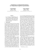
Figure 2: Updating a conflict graph after itemsets
A and E are used to compose a transaction

Proof. We prove the theorem by constructing a database
that matches the requirements
2
. Without loss of generality,
assume we have to generate 1/s% transactions. (To gener-
ate an artificial database of n transactions, we replicate the
database ns% times.) Thus, an itemset that is contained in
at least one transaction is frequent.
A transaction is generated by adding AFI itemsets to it.
Intuitively, we want to add as many AFI itemsets without
bringing in any AII itemsets to the transaction. By Theo-
rem 2, this can be achieved by ensuring that no conflicting
AFI itemsets are added to the transaction. To do so, we
maintain two sets Q
+
and Q
−
, which are initially empty.
Q
+
keeps track of the itemsets that have been added to the
transaction, and Q
−
keeps track of the itemsets that conflict
with any itemsets in Q
+
. We randomly pick an itemset v
in AFI , put v in Q
+
and all its neighbors N(v) to Q

−
. We
repeat this process until AFI is partitioned into:
• Q
+
: Every itemset in Q
+
does not conflict with any
other itemsets in Q
+
.
• Q
−
: Every itemset in Q
−
conflicts with at least one
itemset in Q
+
.
The first transaction is given by

x∈Q
+
x. Since all item-
sets in Q
+
are now frequent (recall that we only need a sup-
port count of 1 to make an itemset frequent), subsequent
transactions need not contain them. We remove all itemsets
in Q

+
from AFI and update the conflict graph removing
the corresponding nodes and their associated edges. Let
G

= (V

, E

) be the updated conflict graph and c

x
be the
conflict index of any node x in G

.
For any node x in G

, we know that x ∈ Q
−
. Hence, there
must exist a neighbor of v in the original conflict graph G
that has been removed in G

. So, c

x
≤ c
x
− 1. This implies

CI (G

) ≤ CI(G)−1. The conflict index of the conflict graph
is reduced by at least 1.
To generate another transaction, we repeat the above pro-
cedure. Finally, the conflict index of the conflict graph will
be reduced to 0. This implies that the itemsets remaining in
AFI are conflict-free. We then generate a transaction that
includes all these remaining itemsets. Note that in the whole
process, we have generated at most CI (G) + 1 transactions.
Recall that we have to generate a database of 1/s% trans-
actions. So if 1/s% ≥ CI(G) + 1, all the transactions gener-
ated in the above procedure can be accommodated. We can
replicate some of the generated transactions so that the to-
tal number of them is 1/s%. As a result, if CI (G) ≤
1
s%
−1,
the procedure correctly generates a database with the de-
sired property. Hence, the theorem.
2
We refer to this construction method “baseline construc-
tion” in the rest of the paper.
Let us use an example to illustrate this baseline con-
struction procedure. Consider the itemset pattern (AFI =
{A, B, C, D, E}, AII = {AB, BC, BD, CD, DE, CE}), whose
conflict graph G is shown in Figure 2 (left). CI (G) = 3. To
generate the first transaction, we pick an AFI itemset, say
A, and get Q
+

= {A}, Q
−
= {B}. Since {C, D, E} in AFI
are not yet partitioned, we repeat the process and pick, say,
E, resulting in Q
+
= {A, E}, Q
−
= {B, C, D}. Now, AFI
is partitioned into Q
+
and Q
−
, therefore transaction AE is
generated. The conflict graph is updated by removing A and
E (see Figure 2 (right)), which has a smaller conflict index
(CI (G

) = 2). The process is repeated for the remaining
AFI itemsets ({B, C, D}) and eventually the baseline con-
struction method generates three more transactions: B, C,
and D.
Theorem 3 states a sufficient condition under which an
itemset pattern is valid. We call this condition valid-pattern
condition or vp-condition for short. Our next task is to gen-
erate such a valid pattern.
4.3 Valid itemset pattern generation
Recall that itemsets in AFI and AII are included in an
audit environment and are used to verify the mining result.
So, a larger AFI ∪ AII leads to a higher verification confi-

dence, but also a longer verification time.
We assume that p
owner
has some rough information of the
number of frequent itemsets and the number of itemsets in
the negative border of his database (i.e., |L| and |B
−
(L)|).
For example, these figures could be obtained from a previous
mining exercise, or from the mining result of a small sample
of the database. The owner then selects a fraction 0 <
f ≤ 1 and set the target sizes of AFI and AII to f
AFI
=
f · |L| and f
AII
= f · |B
−
(L)|, respectively. (Here, |L| and
|B
−
(L)| are rough estimates.) The owner thus controls the
tradeoff between verification accuracy and speed through f.
3
We now briefly describe the high-level idea of a procedure
for generating a valid itemset pattern (AFI , AII ) such that
|AFI | ≥ f
AFI
and |AII | ≥ f
AII

. A pseudocode showing the
details of the procedure is listed in the Appendix.
First, we create a set of artificial items, I
A
.
4
The proce-
dure attempts to add itemsets to AII until both AFI and
AII are “big enough”. We randomly generate an itemset
J ⊆ I
A
that is not already in AII and add J to AII . Since
itemsets in AII are used to verify the negative border of the
mining result, we add all immediate subsets of J to AFI
(so as to make sure that J is in the negative border of the
returned result if p
miner
is not malicious). For example, if
J = ABC, we add AB, BC, AC to AFI . If the resulting
(AFI , AII ) does not satisfy the vp-condition, we roll back
the insertion of J. Otherwise, we compute the negative bor-
der of (the updated) AFI . Itemsets in this negative border
can be added to AII (if not already there). We check the vp-
condition while adding each of them. If that is not satisfied,
we roll back that insertion.
3
If p
owner
wishes to perform mining with various support
thresholds (which would result in various numbers of fre-

quent itemsets), he should generate the AFI and AII using
the minimum of these support thresholds, as the AFI and
AII generated for lower thresholds include the correspond-
ing sets generated for a higher threshold.
4
The initial size of I
A
is not critical, since our procedure
will dynamically adjust it. A reasonable initial size would
be the size of the largest itemset in the estimated B
−
(L).
In the above procedure, if J is successfully added to AII ,
we generate another J from I
A
and repeat the steps. On the
other hand, if the insertion of J is rolled back, we create a
new artificial item α, put α in I
A
, replace an “old” item in J
by α, and attempt to insert J into AII again using the above
procedure. The reason for such a replacement strategy is
that if |J| = k, then in the worst case, after k attempts
of inserting J into AII , J will be composed of purely new
items. In that case, inserting J into AII will not violate the
vp-condition and the insertion is guaranteed to be successful.
The replacement strategy thus ensures that the construction
procedure terminates within a finite amount of time.
4.4 Database generation
Given a valid itemset pattern (AFI , AII ), the next step is

to generate an artificial database
ˆ
T such that all itemsets in
AFI are frequent and all itemsets in AII are infrequent. A
simple approach to generate such a database is to follow the
baseline construction method described in the proof of The-
orem 3. However, such a database has the special property
that all itemsets in AII have 0 supports and the supports
of the itemsets in AFI are very close to the support thresh-
old. This is undesirable because a malicious miner might
deduce the artificial items and eliminate the chance of being
detected, by avoiding to change their supports.
To improve the robustness of the audit environment, we
add more randomness in the generation of an artificial database.
In particular, itemsets in AII could be given small, but non-
zero supports. The supports of itemsets in AFI are also
given more variation. In this subsection, we describe one
such artificial database generation method.
We start with a few definitions. Each itemset x ∈ AFI
is associated with a weight, denoted by w(x). Intuitively,
w(x) indicates the minimum number of transactions in
ˆ
T
that should contain x. So, w(x) = |
ˆ
T | · s% because there
have to be at least |
ˆ
T | · s% transactions in
ˆ

T that contain x
for x to be frequent.
Definition 8. (Weighted conflict index) Given a conflict
graph G = (V, E) and a weight function w(), let N(x) de-
note the set of neighbors of vertex x. The weighted conflict
index wc
x
of x is the sum of the weight of x and the total
weights of its neighbors, i.e., wc
x
= w(x) +

y∈N (x)
w(y).
The weighted conflict index of G, denoted by WCI (G), is
max
x∈V
wc
x
.
Theorem 4. Given an itemset pattern (AFI , AII ), a
weight function w(), and an integer n, there exists an ar-
tificial database
ˆ
T of n transactions such that (1) for each
x ∈ AFI , the support of x ≥ w(x) and (2) all itemsets in
AII have 0 supports, if both of the following conditions hold:
1. AFI and AII satisfy the monotonicity property.
2. WCI (G) ≤ n.
Proof. We give a sketch of a proof that is very simi-

lar to the construction proof we described in Theorem 3.
Similar to the baseline construction method, we partition
AFI into Q
+
and Q
−
. A transaction

x∈Q
+
x is gener-
ated. The weight function is updated to w

() as follows:
w

(x) = w(x) − 1, ∀x ∈ Q
+
; w

(x) = w(x), ∀x ∈ Q
−
.
That is, the weight of each itemset included in the gen-
erated transaction is reduced by 1. We update the conflict
graph G = (V, E) to G

= (V

, E


) such that all vertices x
with w

(x) = 0 are removed from G together with all their
associated edges. Also, denote the weighted conflict index of
any x ∈ G

by wc

x
. We note that for each x ∈ V

, if x ∈ Q
+
,
then all its neighbors must be in Q
−
. Since w

(x) = w(x)−1
and the weights of all x’s neighbors are unchanged, we have
wc

x
= wc
x
− 1. Moreover, if x ∈ Q
−
, then there must ex-

ist at least one neighbor y of x such that y ∈ Q
+
. Since
w

(y) = w(y) − 1, we have wc

x
≤ wc
x
− 1. As a result,
WCI (G

) ≤ WCI(G) − 1.
We repeat this process of transaction generation. For each
transaction generated, the weighted conflict index of the
graph is reduced by at least 1. Eventually, the conflict graph
is reduced to the null graph, after at most WCI (G) trans-
actions have been generated. Since each itemset x ∈ AFI
has its weight reduced from w(x) to 0 in the process, w(x)
transactions that contain x must have been generated. If
WCI (G) ≤ n, an artificial database of n transactions that
satisfies the minimum support requirement can be obtained
by taking all the generated transactions and replicate some
of them until we get n transactions.
We now briefly describe an algorithm for generating an ar-
tificial database
ˆ
T such that itemsets in AII could have non-
zero (but infrequent) supports, and the itemsets in AFI are

frequent with a wider variation of support counts. We high-
light the important steps; a detailed pseudo code is listed
in the Appendix. We assume that AFI and AII satisfy the
monotonicity property.
First, for each x ∈ AFI , we set w(x) = n · s% where n is
the number of artificial transactions to be generated. Also,
for each y ∈ AII , we set a quota, q
y
< n · s%. Intuitively,
q
y
specifies how many generated transactions can contain
y at most. We randomly pick an itemset z
1
∈ AFI and
randomly pick a number of other items in I
A
, say z
2
⊂ I
A
,
to form a transaction
ˆ
t = z
1
∪ z
2
. For each x ∈ AFI , if
x ⊆

ˆ
t, we reduce its weight, w(x), by 1. For each y ∈ AII ,
if y ⊆
ˆ
t, we reduce its quota, q
y
, by 1. If q
y
< 0, we know
that taking
ˆ
t will cause some AII itemset to be frequent, so
transaction
ˆ
t is discarded. Otherwise, we check the condition
(WCI (G) ≤ n − 1) with respect to (AFI , AII , (updated)
w(), n − 1). If the condition is satisfied, then by Theorem 4,
we know that it is possible to generate a database that,
together with
ˆ
t, satisfies all the support constraints. We
thus include
ˆ
t in
ˆ
T and repeat the above process. On the
other hand, if the condition is not satisfied, we discard
ˆ
t and
generate another transaction. When a generated transaction

ˆ
t is inserted to
ˆ
T , we increment the support count of each
subset u of
ˆ
t if u ∈ AFI or u is a subset of an itemset that
is in AFI .
To ensure that the procedure terminates in a finite amount
of time, we use a control parameter b. If we have discarded
transactions b consecutive times without successfully gener-
ating one, we fall back to the baseline construction method
to generate the next transaction.
After the database generation concludes, our audit envi-
ronment consists of (i) AII , (ii) AFI , and (iii) the support
counts of all itemsets in AFI and their subsets. The lat-
ter set is used to verify whether the supports of returned
itemsets are not modified by a malicious action of p
miner
.
4.5 Security and cost analysis
In this section, we analyze the effectiveness of AIP in
guarding against malicious actions by p
miner
and the com-
putational cost of applying AIP at p
owner
.
Due to the random generation of transactions in the ar-
tificial database, the supports of artificial itemsets vary and

follow a similar distribution as the supports of the original
itemsets. Therefore, p
miner
is expected not to be able to
distinguish between original itemsets and artificial ones in
the outsourced database. As a result, the malicious actions
performed by p
miner
(described in Section 3.1) may apply
to artificial and/or actual itemsets.
Suppose p
miner
performs a malicious action on an itemset
x; x may be (i) an itemset in the original database; or (ii)
an itemset in AF I or AII; or (iii) an itemset that is nei-
ther from the original database nor in AF I ∪ AII (e.g., x
contains both original as well as artificial items). Our au-
dit environment will fail to detect actions on type-(i) item-
sets. In addition, p
miner
’s gain on such actions will be pos-
itive, since they will affect the mining result of the original
database. On the other hand, p
miner
’s actions on type-(ii)
and type-(iii) itemsets do not affect the actual results and
bring no gain to him. Moreover, if x is of type (ii), the ac-
tion can be detected by our audit environment and p
miner
may be caught and penalized. Let the gain φ(A

i
) by a ma-
licious action A
i
be h > 0 if A
i
is performed on a type-(i)
itemset. Note that φ(A
i
) = 0 for actions on any itemset
of another type. For simplicity, we assume no malicious
actions are performed on type-(iii) itemsets, since p
miner
does not gain from such actions and the actions cannot be
detected. Let m = |L

B
−
(L)|, where L is the true set of
frequent itemsets in the original database (i.e., type-(i) item-
sets). Let n be the number of type-(ii) itemsets. If p
miner
performs j malicious actions and returns R

, the probabil-
ity p of being caught is equal to the probability that he
picks at least one of the n balls in a set of m + n balls. So,
p = 1−Π
j−1
i=0

m−i
m+n−i
= 1−
m!
(m+n)!
×
(m+n−j)!
(m−j)!
. If p
miner
is not
caught (by not picking any of the n balls), the expected gain
is jh. So, EG(R

) = jh(1 − p) − pρ. If EG(R

) is negative
for all values of j and R

, the malicious miner is expected to
lose. Therefore, p
miner
is forced to act honestly and returns
the correct and complete results. Using this analysis as a
guideline, we can derive the required number of artificial
itemsets to be planted in order to protect the mining result.
In Section 5, we perform an experimental security analysis
and demonstrate that AIP is very effective in practice.
The cost of AIP at p
owner

consists of three parts:
a. Itemset pattern generation. The dominating cost fac-
tor in itemset pattern generation is the maintenance of the
conflict graph. When an AII itemset is added, we also add
its immediate subsets to AFI (those that are not already
there). Then, for every pair of itemsets in the updated
AFI , which are not already in conflict, we need to check
whether they are now in conflict due to the insertion of the
new AII itemset. There are |AFI |
2
such pairs in the worst
case. Therefore each AII itemset insertion costs O(|AFI |
2
)
and the total cost of the itemset pattern generation phase is
O(|AII | × |AFI |
2
). Despite this seemingly large complexity,
the generation process is independent of database size and
it is expected to be cheap compared to database scans for
small AII and AFI . Our experiments (see Section 5) show
that this cost is indeed insignificant.
b. Database generation. When a transaction
ˆ
t is gen-
erated, we have to update the quotas (weights) of all AII
(AFI ) itemsets that are included in
ˆ
t. This requires O(|AFI |+
|AII |) time. In addition, for each such AFI itemset y, we

need to decrement the weighted conflict index wc
x
for each
neighbor x of y in the conflict graph. In the worst case,
there are 1/s% such neighbors. Therefore the cost of gener-
ating
ˆ
t is O(
|AFI |
s%
+ |AII |). In the worst case, b unsuccessful
trials could be attempted before a transaction
ˆ
t is success-
fully generated. Hence, the maximum number of transac-
tions tested is b × |
ˆ
T |. Overall, the cost of generating
ˆ
T is
O(b × (
|AFI |
s%
+ |AII |)|
ˆ
T |). We remark that the bounds men-
tioned about in our worst-case analysis are very loose. Also,
we will discuss an optimization method in Section 4.6 that
greatly reduces the database generation time. As we will
see later in our experimental results, the database genera-

tion time is much smaller than the mining time in practice.
c. Detection of malicious actions. The owner detects ma-
licious actions by (i) checking whether any AII itemsets are
returned by the miner as frequent and (ii) for all itemsets in
AFI and the subsets thereof, comparing the support counts
given by p
miner
with the stored counts prepared in the audit
environment, during the database generation phase. The to-
tal cost of this phase is O(k), where k is equal to the number
of AII itemsets plus the number of support counts recorded
in the audit environment. Again, our experimental results
show that this verification cost is small.
4.6 Reducing the cost of database generation
In Section 4.4 we discussed how to generate an artifi-
cial database
ˆ
T . The number of transactions generated |
ˆ
T |
equals the size of the original database T . We remark that
it is not necessary to generate such a large number of ar-
tificial transactions. Recall that the requirement of
ˆ
T is to
ensure that all AFI itemsets are frequent while all AII item-
sets are infrequent. A more efficient way to generate
ˆ
T is
to generate a smaller database


T
D
that satisfies the AFI
and AII constraints and replicate

T
D
to obtain |
ˆ
T | artificial
transactions. For example, we can generate a

T
D
of 1,000
transactions, replicate it 100 times to obtain a
ˆ
T of 100,000
transactions. A minor problem of this method is that the
support counts of artificial itemsets would all be multiple
of |
ˆ
T |/|

T
D
|. To avoid frequency attack, we add variability
to the support counts. This can be achieved by generating
another small database


T
V
that satisfies the AFI and AII
constraints. Database
ˆ
T is then obtained by replicating

T
D
a number of times followed by adding the transactions in

T
V
.
With this approach, we are generating two small databases

T
D
and

T
V
instead of a large one
ˆ
T . The database genera-
tion process is thus much faster.
An interesting issue is how to pick the sizes of

T

D
and

T
V
.
Let r be the number of times

T
D
is replicated. We have
|

T
D
| × r + |

T
V
| = |T | (1)
Since the purpose of

T
V
is to inject variations to the support
counts (which are originally all multiples of r), ideally, we
want the support counts of the itemsets found in

T
V

to cover
at least the range [1 . . . r]. An easy way to ensure that is to
make r smaller than the support count threshold of

T
V
. So
if we consider the itemsets in

T
V
(which include those fre-
quent ones), the support counts can cover the range [1 . . . r].
Hence, we set
|

T
V
| × s% ≥ r (2)
Substituting Eq. 2 into Eq. 1, we get |

T
V
|(1 + s%|

T
D
|) ≥
length of s = 1 s = 2 s = 3
itemset |L

i
| |B
−
i
(L)| |L
i
| |B
−
i
(L)| |L
i
| |B
−
i
(L)|
1 310.0 690.0 179.8 820.2 99.0 901.0
2 590.6 47305.8 136.6 15937.6 38.8 4812.2
3 664.6 807.4 110.8 44.2 19.0 8.0
4 383.2 127.0 60.6 2.4 8.0 0.0
5 156.0 3.4 14.0 6.0 5.6 0.0
6 44.2 3.4 0.8 0.2 0.0 0.0
7 4.2 0.2 0.0 0.0 0.0 0.0
Total 2152.8 48937.2 502.6 16810.2 170.0 5721.2
Table 1: Average values of |L
i
| and |B
−
i
(L)| under
different support threshold (s%)

|T |. Therefore, determining |

T
D
| and |

T
V
| becomes a con-
straint optimization problem with the objective of minimiz-
ing |

T
D
| + |

T
V
| (i.e., the total number of transactions to be
generated). For example, if |T | = 1M and s = 5, the opti-
mal solution is |

T
D
| = 5000 and |

T
V
| = 5000 for an integer
r.

5. EXPERIMENTAL EVALUATION
In this section we evaluate AIP empirically. We study
its effectiveness in detecting malicious actions and the cost
they induce to both the data owner and the data miner.
We implemented all the programs for AIP using C++. Ex-
periments were performed on an Intel Core 2 Duo 2.66GHz
computer with 2 GB RAM running Windows.
5.1 Settings
In the experiments, we generated 5 transactional databases
using the IBM data generator [6] with the same set of pa-
rameters (|I| = 1000, average transaction length |t| = 10).
The databases differ in size, from 100k transactions to 500k
transactions. Since the same set of parameters are used in
generating the databases, the different databases have sim-
ilar numbers of frequent itemsets (|L|) and similar sizes of
their negative borders (|B
−
(L)|). Table 1 shows the average
number of length-i frequent itemsets, denoted by |L
i
| and
the average number of length-i itemsets that are in the neg-
ative border, denoted by |B
−
i
(L)|, for the 5 databases under
3 different support thresholds (s = 1%, 2%, 3%).
As we have discussed, in AIP, we need to provide a rough
estimate of the sizes of AFI and AII (in order to generate
AFI and AII ). In our experiment, we set |AFI | = v · |L|

and |AII | = v · |B
−
(L)|, for some fractional value v.
5.2 Effectiveness in detecting malicious actions
We first study the probability that a malicious miner is
detected/caught by AIP. If the miner returns an accurate
result L, a perfect verifier will have to check the support
counts of all itemsets in L ∪ B
−
(L) (see Section 4). So,
if the miner performs e · (|L| + |B
−
(L)|) malicious actions,
loosely speaking, the miner is perturbing a fraction e of the
result. In our first experiment, the miner randomly per-
forms e · (|L|+ |B
−
(L)|) malicious actions. We apply AIP to
verify the result and take note of whether a malicious act is
detected. We repeat this experiment 5,000 times and record
the probability (p) that the malicious miner is caught by AIP
over the 5,000 sample runs. Figure 3 plots this probability
against e for v ranges from 0.5% to 3%. In this experiment,
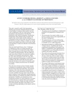
we set s = 1 and |T | = 100k.
From the figure, we see that p increases with e — the
more perturbation done, the more likely a malicious miner
0
20
40
60

80
100
0 0.2 0.4 0.6 0.8 1
e (%)
Detection probability p (%)
v=3%
v=2.5%
v=2%
v=1.5%
v=1%
v=0.5%
Figure 3: Probability that a malicious miner is
caught (p) vs. e
is caught. Also, a larger v (i.e., more AFI and AII itemsets
are used for verification) gives a larger p. Moreover, the
detection probability p is almost 100% for all v values even
when the miner has perturbed as little as e = 0.6% of the
result. The following 1%-1% rule: “By verifying 1% of the
result (v = 1%), a malicious miner that has perturbed more
than 1% of the result (e > 1%) is almost always caught,”
can be seen as a conservative statement on the effectiveness
of AIP in this experiment.
Recall that in Section 2 we define the expected gain (EG)
of a malicious miner. An interesting question is what Fig-
ure 3 can tell us about such expected gains. Let g be the
gain obtained by the miner for each malicious action per-
formed and ρ be the penalty suffered by the miner if it gets
caught. If the miner performs N malicious actions, we have
EG = (1− p)Ng −pρ. In order for such malicious acts to be
profitable, we need EG > 0, which implies

ρ
g
< N·
1−p
p
. Now
consider Figure 3. Given e, we get N = e · (|L| + |B
−
(L)|).
For a given v, the corresponding curve in Figure 3 gives us a
p value. For example, in our experiment, with e = 0.4%
and v = 1%, we get N = 200 and p = 0.976. Hence,
N ·
1−p
p
= 4.92. In other words, the gain per each mali-
cious act has to be at least
1
4.92
of the penalty suffered in
order for EG > 0. However, as we have argued, ρ should be
much much larger than g in practice. Therefore, under AIP,
malicious actions are simply non-profitable. Result integrity
can thus be strongly enforced.
5.3 Cost analysis
We study the efficiency of AIP. In particular, we study the
cost of generating itemset patterns, the cost of generating
an artificial database, the cost of verification, and the cost
of the miner in mining a transformed (and larger) database.
First, Table 2 shows the execution time of the classic Apri-

ori algorithm when applied to our databases under different
support thresholds
5
. We remark that any practical verifica-
tion scheme should not cost the data owner more time than
those listed in the table.
Generation of a valid pattern Section 4.3 described
5
We use Apriori here just to illustrate the typical mining
times if the data owner chooses to perform mining itself
using off-the-shelf packages instead of outsourcing the task.
Other more efficient mining algorithms can also be applied.
For the latter case, the numbers shown in Table 2 will be
smaller, although we expect that the numbers will be of
similar magnitude.
support Database size
threshold 100k 200k 300k 400k 500k
1% 186.6s 383.8s 569.1s 761.9s 944.3s
2% 67.3s 135.7s 203.5s 271.5s 339.3s
3% 24.8s 49.5s 74.2s 98.9s 123.6s
Table 2: Execution time of Apriori
0
0.5
1
1.5
2
2.5
0 0.5 1 1.5 2 2.5 3
v (%)
Execution time (s)

s=1
s=2
s=3
Figure 4: Time taken to generate a valid pattern
our algorithm for generating a valid pattern (AFI , AII ).
Figure 4 shows the execution time of the algorithm as v
changes from 0.5% to 3%. Three lines are shown corre-
sponding to three support thresholds.
From the figure, we see that as v increases, the time taken
to generate a valid pattern becomes longer. This is because
a larger v implies a larger AFI and a larger AII . More
itemsets have to be generated and that takes longer. Also,
generating itemsets when AFI and AII are already big is
harder. This causes more rollbacks and retries during the
generation process. In any case, the pattern generation time
is very small compared with the mining time (Table 2). For
example, when s = 1% and v = 3, pattern generation takes
about 2 seconds. The execution time is negligible for higher
support thresholds.
Generation of an artificial database Given a valid
pattern (AFI , AII ) we generate an artificial database. Sec-
tion 4.4 described our basic algorithm for generating arti-
ficial transactions and Section 4.6 described an optimiza-
tion that generates two small databases instead of a big
one. Figure 5 shows the database generation time using
the optimized method under different combinations of v and
database sizes |T |. In this experiment, the support threshold
is 2%.
From the figure, we observe that a larger v causes the
s=2 db1 gen time s=2

v 100k 200k 300k 400k 500k v 100k
0.5 0.0171 0.0265 0.03122 0.0359 0.0406 0.5 0.0171
1 0.0279 0.0405 0.0484 0.0529 0.0626 1 0.0279
1.5 0.0295 0.0421 0.061 0.0547 0.0626 1.5 0.0295
2 0.0312 0.047 0.0625 0.0707 0.078 2 0.0312
2.5 0.0439 0.0596 0.0735 0.0843 0.0984 2.5 0.0439
3 0.0469 0.0719 0.0844 0.0984 0.1094 3 0.0469
s=2 total time s=2
v 100k 200k 300k 400k 500k v 100k
0.5 0.399128 0.769607 1.163565 1.617596 1.942992 0.5 0.35
1 0.424657 0.803214 1.169349 1.672392 2.058285 1 0.339
1.5 0.439785 0.822421 1.209774 1.696788 2.049877 1.5 0.336
2 0.461113 0.857327 1.245099 1.833884 2.13487 2 0.339
2.5 0.496742 0.892834 1.279123 1.80548 2.212662 2.5 0.3343
3 0.52397 0.949641 1.370848 1.951376 2.357554 3 0.3406
s=2 count time
v 100k 200k 300k 400k 500k 0.343
0.5 0.014928 0.021307 0.026125 0.030196 0.033792
1 0.029857 0.042614 0.052249 0.060392 0.067585
1.5 0.044785 0.063921 0.078374 0.090588 0.101377
2 0.059713 0.085227 0.104499 0.120784 0.13517
2.5 0.074642 0.106534 0.130623 0.15098 0.168962
3 0.08957 0.127841 0.156748 0.181176 0.202754
100 200 300 400 500
67.25 135.656 203.531 271.454 339.281
s=2 total time
v 500k 400k 300k 200k 100k
0.5 1.875928 1.558107 1.461714 0.791142 55%
1 1.879856 1.603213 1.503427 0.819285 45%
1.5 1.930784 1.69432 1.575141 0.893427 48%

2 2.009712 1.755426 1.678855 0.92057 0.533427
2.5 2.044641 1.829533 1.718569 0.947712 0.663784
3 2.110569 1.889639 1.807282 1.038855 0.575141
|T|
0
0.5
1
1.5
2
2.5
0 0.5 1 1.5 2 2.5 3
v (%)
Execution time (s)
500k
400k
300k
200k
100k
Figure 5: Time taken in database generation for var-
ious v and database sizes; s = 2
v 500k
0.5 47.51784
1 64.84301
1.5 69.34311 mining tim
e
339.281
2 81.66181 0.5 500.5 47.51784
2.5 92.11597 1.5 574.549 69.34311
3 98.48061 2.5 651.813 92.11597
45

65
85
105
0 0.5 1 1.5 2 2.5 3
v (%)
Mining overhead (%)
Figure 6: Mining overhead for various v; s = 2 and
|T | = 500k
database generation process to take slightly more time. This
is because a larger v means larger AFI and AII . The
weighted conflict graph G is thus larger. The cost of up-
dating G and checking the condition WCI (G) ≤ n (see Sec-
tion 4.4) is slightly higher.
Also, the larger the database is, the higher is the genera-
tion time. This is because a larger |T | implies a larger |T
D
|
and a larger |T
V
|. So the two small databases we generate
are bigger, leading to a longer generation time.
Again, we have argued that v = 1% is generally good
enough to achieve a high detection probability. In that case,
Figure 5 shows that database generation takes about 2 sec-
onds to complete (even for a database of 500k transactions).
Compare that to the numbers shown in the second row of
Table 2 (for support threshold = 2%), the cost of generating
a database is relatively insignificant.
Verification Given a returned result L


, the verification
process verifies the support counts of itemsets in (AFI ∪
AII ) ∩ (L

∪ B
−
(L

)) by comparing the stored count values
against those returned in the result. In our experiment, it
takes less than 1 ms.
Mining overheads at service provider Next, we study
how much additional mining time the miner has to pay. Note
that the miner has to mine a larger (horizontally extended)
database with additional artificial items. We compute the
ratio of the additional mining time with AIP and the mining
time without AIP
6
. Figure 6 shows this ratio for the case |T|
= 500k and s = 2. For example, the figure shows that when
v = 2%, the additional mining overhead is about 80% of the
original mining time; for v = 1%, the overhead is reduced to
about 65%. In the latter case, the average transaction size
increases from 10.08 items per transaction in the original
database to 12.26 items in the database submitted to the
miner; the database size increases from 24.6MB to 28.7MB;
and the number of frequent itemsets increases from 501 to
639. In general, a larger v leads to a higher mining overhead
at p
miner

. This is because a larger v causes more artificial
items and itemsets to be included in the database. The
mining time is thus higher. We remark that this overhead
should be manageable by the service provider.
6. CONCLUSIONS AND FUTURE WORK
In this paper we put forward the integrity problem in out-
sourcing the task of frequent itemset mining. We established
6
We assume p
miner
uses the Apriori algorithm in this exper-
iment. We remark that AIP is independent of the mining
algorithm the miner uses. We expect that the overhead in-
duced by AIP is mostly dependent on the additional itemsets
and artificial transactions introduced by AIP, instead of on
the mining algorithm employed.
a formal framework of the problem with a definition of a set
of malicious actions that a malicious service provider might
perform. We have shown theoretically that a full verifica-
tion of the correctness and completeness of a mined result
requires examination of the support counts of all itemsets in
the result plus those in the negative border of the result. The
high cost of such verifications leads to the development of a
sampling approach under the concept of an audit environ-
ment. We proposed the artificial itemset planting technique
for preparing an audit environment. We explained how AIP
works through a set of theorems. A malicious miner cannot
benefit from performing any of the malicious actions and
thus the returned mining result is both correct and com-
plete with a high confidence. We evaluated our algorithms

through a series of experiments. Our technique is shown to
be both effective and efficient at p
owner
. In the future, we
will work on reducing the mining overhead and make it a
controllable factor by integrating AIP and sampling tech-
niques on original database, which do not inject additional
data and hence do not bring in additional mining effort at
p
miner
.
7. REFERENCES
[1] R. Agrawal and R. Srikant. Fast algorithms for mining
association rules. In VLDB, 1994.
[2] S. Brin, R. Motwani, J. D. Ullman, and S. Tsur.
Dynamic itemset counting and implication rules for
market basket data. In SIGMOD, 1997.
[3] X. Chen and M. Orlowska. A further study on inverse
frequent set mining. In ADMA, 2005.
[4] G. Grahne and J. Zhu. Efficiently using prefix-trees in
mining frequent itemsets. In FIMI, 2003.
[5] H. Hacigumus, B. Iyer, and S. Mehrotra. Providing
database as a service. In ICDE, 2002.
[6] IBM Almaden Research Center. Synthetic data
generation code for association and sequential
patterns.
[7] F. Li, M. Hadjieleftheriou, G. Kollios, and L. Reyzin.
Dynamic authenticated index structures for
outsourced databases. In SIGMOD, 2007.
[8] F. Li, K. Yi, M. Hadjieleftheriou, and G. Kollios.

Proof-infused streams: Enabling authentication of
sliding window queries on streams. In VLDB, 2007.
[9] G. S. Manku and R. Motwani. Approximate frequency
counts over data streams. In VLDB, 2002.
[10] T. Mielikainen. On inverse frequent set mining. In
PPDM, 2003.
[11] H. Pang, A. Jain, K. Ramamritham, and K L. Tan.
Verifying completeness of relational query results in
data publishing. In SIGMOD, 2005.
[12] S. Papadopoulos, Y. Yang, and D. Papadias. CADS:
Continuous authentication on data streams. In VLDB,
2007.
[13] G. Ramesh, W. A. Maniatty, and M. J. Zaki. Feasible
itemset distributions in data mining: theory and
application. In PODS, 2003.
[14] G. Ramesh, M. J. Zaki, and W. A. Maniatty.
Distribution-based synthetic database generation
techniques for itemset mining. In IDEAS, 2005.
[15] R. Sion. Query execution assurance for outsourced
databases. In VLDB, 2006.
[16] W. K. Wong, D. W. Cheung, E. Hung, B. Kao, and
N. Mamoulis. Security in outsourcing of association
rule mining. In VLDB, 2007.
[17] M. Xie, H. Wang, J. Yin, and X. Meng. Integrity
auditing of outsourced data. In VLDB, 2007.
APPENDIX
Algorithm 1 Pseudo code of database generation
Require: AFI , AII : valid itemset pattern
Require: I
A

: set of items in the artificial database
Require: b : the maximum number of random generation
Require: n : number of transactions to generate
Require: s% : support threshold
{Initialization}
for each itemset x in AFI do
w(x) = n · s%
end for
for each itemset x in AII do
q
x
= r where r < n · s%
end for
{Generate transaction}
for i = 1 to n do
j = 1
repeat
if j > 1 then
roll back updates of w(x) and q
x
end if
if j > b then
generate
ˆ
t by baseline construction
else
r = random integer in [0, |AFI |]
if r = 0 then
z
1

= ∅
else
z
1
= AFI [r] {AFI [r] is the r-th itemset in AFI }
end if
z
2
= random subset of I
A
ˆ
t = z
1
∪ z
2
end if
{Update weights and quotas}
j + +
for each itemset x ∈ AII and x ⊆
ˆ
t do
if q
x
= 0 then
go to next iteration {x is made frequent}
else
q
x
− −
end if

end for
for each itemset x ∈ AFI and x ⊆
ˆ
t do
q
x
= max(0, q
x
− 1)
end for
until WCI (G) < n − i
end for
Algorithm 2 Pseudo code of valid pattern generation
Require: f
AFI
[i] : a size m array specifying the target num-
ber of size i itemset in AFI
Require: f
AII
[i] : a size n array specifying the target num-
ber of size i itemset in AII
Require: s% : support threshold
{Initialization}
AII = AFI = ∅, G = (∅, ∅)
I
A
= a set of n items
{Generate AII }
for i = n to 1 do
count = |{x | x ∈ AII and |x| = i}|

while count < f
AII
[i] do
generate an itemset x by randomly pick i items in I
A
such that x ∈ AII
AII = AII

{x}
j = 1
Y = {y | y ⊂ x and |y| = i − 1 and ∀z ∈ AFI , y ⊆ z}
AFI = AFI

Y
update G accordingly
while vp-condition is not satisfied do
roll back adding of x to AII and Y to AFI
generate a new item p
x[j] = p {x[j] is the j-th item in x}
AII = AII

{x}
I
A
= I
A

{p}
Y = {y | y ⊂ x and |y| = i − 1 and ∀z ∈ AFI , y ⊆
z}

AFI = AFI

Y
update G accordingly, j + +
end while
count + +
{We include the new members in B
−
(AFI ) to AII }
∆B
−
(AFI ) = {z | ∀s ⊂ z, ∃w ∈ AFI , s ⊆ w and
∃s ⊂ z, ∀w ∈ AFI − Y, s ⊆ w}
for each itemset z ∈ ∆B
−
(AFI ) do
AII = AII

{z}
if vp-condition is not satisfied then
roll back adding of z
else
if |z| = i then
count + +
end if
end if
end for
end while
end for
{Generate AFI }

for i = m to 1 do
count = |{x | ∃y ∈ AFI, x ⊆ y and |x| = i}|
while count < f
AFI
[i] do
generate an itemset x by randomly pick i items in I
A
such that ∀y ∈ AFI , x ⊆ y
AFI = AFI

{x}
j = 1
update G accordingly
while vp-condition is not satisfied do
roll back adding of x to AFI
generate a new item p
x[j] = p
AFI = AFI

{x}
I
A
= I
A

{p}
update G accordingly, j + +
end while
count + +
end while

end for