TRANSFER PRICING FOR COORDINATION AND PROFIT ALLOCATION pptx
Bạn đang xem bản rút gọn của tài liệu. Xem và tải ngay bản đầy đủ của tài liệu tại đây (1003.7 KB, 20 trang )
Australian Journal of Business and Management Research Vol.1 No.6 [07-26] | September-2011
7
TRANSFER PRICING FOR COORDINATION AND PROFIT ALLOCATION
Jan Thomas Martini
Department of Business Administration and Economics
Bielefeld University, Germany
E-mail:
ABSTRACT
This paper examines coordination and profit allocation in a profit-center organization using a single transfer
price. The model includes compensations, taxes, and minority interests of two divisions deciding on capacity and
sales. The analysis covers arm’s length transfer prices which are either administered by central management or
negotiated by the divisions. Administered transfer prices refer to past transactions and therefore maximize
firm-wide profit net of divisional compensations, taxes, and minority profit shares only for given decentralized
decisions. From an ex-ante perspective, it is shown that adverse effects on coordination may result in inefficient
divisional profits of which all stakeholders suffer. We motivate a positive effect of advance pricing agreements,
intra-firm guidelines, and restrictive treatments of changes in the firm’s accounting policy. By contrast,
negotiations ignore compensations, taxes, and minority shares but yield efficient divisional profits. Negotiations
seem compelling as they perfectly reflect the arm’s length principle. Moreover, common practices such as
arbitration or one-step pricing schemes allow the firm to engage in manipulation at the expense of other
stakeholders.
Keywords: Transfer Pricing, Coordination, Profit Allocation, Managerial Accounting, Taxation, Financial
Reporting.
1. INTRODUCTION
Transfer prices are valuations of products within a firm and represent a common and important instrument of
managerial accounting, financial accounting, and taxation. Most of the objectives ascribed to transfer prices are
captured by the functions of coordination and profit allocation. For coordinative purposes, transfer prices affect
performance measures of divisional managements in decentralized organizations.
1
In accordance with the transfer
pricing literature and empirical evidence, we base our argumentation on profit-center organizations. The
coordinative effect stems from the fact that transfer prices are a determinant of the profits of vertically integrated
divisions. While absolute or relative levels of divisional profits are secondary to the coordination of decentralized
managements maximizing their profits, for profit allocation, transfer prices are explicitly employed to quantify a
division‟s „fair‟ contribution to the firm-wide profit. Internally, the allocation of profit might be used for
performance evaluation and resource allocation decisions. However, profit allocation is most important for
external purposes such as financial reporting, profit taxation, and profit distribution. Thus, there are several
stakeholders such as central management, divisional managements, creditors, (potential) shareholders, or tax
authorities having a vital interest in divisional profits.
2
This paper concentrates on a single set of books, i.e., the same transfer price applies for internal as well as for
external purposes. Consequently, the transfer price couples coordination and profit allocation. Ernst & Young
(2003, p. 17) confirm that this situation is descriptive since over 80 percent of 641 multinational parent companies
report that they use the same transfer price for management and tax purposes. The analysis is based on a model of
two vertically integrated divisions whose profits are used for compensation, taxation, and profit distribution. At
the outset, we find that variable compensation, taxes, and profit distributions of a division are proportional to its
profit before compensation, taxation, and profit distribution. Consequently, the divisions only take their gross
profits into account when they take the decision delegated to them although they are assumed to maximize
divisional profits distributable to shareholders, i.e., after compensation and taxation.
On the basis of the arm‟s length principle, we develop two scenarios in which transfer prices are either negotiated
by the divisions before or set by the firm‟s central management after the transaction to be priced. Negotiations on
the transfer price are shown to maximize the firm‟s gross profit from the transaction. Moreover, since divisional
1
We use the term „division‟ for units subordinated to the central management or headquarters of the enterprise as a whole
regardless of their legal form or the (legal) basis of such subordination.
2
Cf. McMechan (2004) and Morris and Edwards (2004) for examples of transfer prices contested on the basis of corporate or
tax law. Further tax court cases are given in Eden (1998, pp. 525–541).
Australian Journal of Business and Management Research Vol.1 No.6 [01-06] | September-2011
8
compensations, taxes, and profit shares are linear in the divisions‟ gross profits, interdivisional negotiations
produce Pareto-efficient transfer prices for any stakeholder of divisional profits such as central management,
divisional managements, shareholders, or tax authorities. However, the firm‟s majority shareholders may benefit
from common transfer pricing practices to manipulate divisional negotiations. In this context, we analyze
arbitration, one-step transfer prices, and the choice of the transfer pricing scheme.
Administered transfer prices are characterized by the minimization of compensations, taxes, and minority profit
shares. Since central management determines the arm‟s length price after the transaction, coordinative effects are
ignored. Thus, it is intuitive that divisional profits are not optimal from an ex-ante perspective. Yet, the model
allows to observe a strong effect of inefficiency: This minimization may lead to Pareto-inefficient divisional
profits so that any stakeholder suffers from inefficiency. This effect exists for a given transfer pricing scheme as
well as for crosschecked schemes. We discuss possibilities for the firm to prevent inefficiency and thereby give an
innovative interpretation of advance pricing agreements and point at benefits from restrictions imposed on the
firm‟s transfer pricing policy.
Related literature is found in the context of transfer pricing for international taxation. Mainly from an economics
or public finance perspective, a sizeable number of contributions examines distortions of production, pricing, or
investment decisions induced by differential tax rates, tariffs, or regulations. The majority of the models assumes
a centralized firm and thereby abstracts from coordinative aspects which is a main ingredient in this model. Papers
pertaining to this strand comprise Smith (2002a), Sansing (1999), Harris and Sansing (1998), Kant (1988; 1990),
Halperin and Srinidhi (1987), Samuelson (1982), and Horst (1971). The idea of a comparative analysis of
divisional profits and transfer pricing schemes found in some of these papers is shared by this paper.
Other papers assume decentralization. Nielsen, Raimondos-Møller, and Schjelderup (2003), Narayanan and
Smith (2000), and Schjelderup and Sorgard (1997) concentrate on transfer prices as strategic devices in
oligopolistic markets. Martini (2008) analyses the firm‟s optimal focus on managerial and financial aspects of
transfer pricing under information asymmetry and a single set of books. Halperin and Srinidhi (1991) analyze the
resale price and the cost plus method when arm‟s length prices are uniquely determined by “most similar
products” traded with uncontrolled parties. Modeling decentralization as a setting, in which divisions negotiate
and contract all decision variables such that, by assumption, consolidated after-tax profit is maximized, they
identify distortions induced by decentralization and tax regulations. Finally, Balachandran and Li (1996) design a
mechanism based on dual transfer prices, and Hyde and Choe (2005), Baldenius, Melumad, and
Reichelstein (2004), Smith (2002b), and Elitzur and Mintz (1996) analyze settings of two sets of books.
This paper analyzes the relevant case of a single set of transfer prices in a decentralized firm including aspects of
compensation, taxation, and profit distribution. The main contributions consist of 1) the efficiency results for
different approaches to the arm‟s length principle including crosschecking, 2) the analysis of the susceptibility of
negotiated transfer prices to common transfer pricing practices such as arbitration and one-step or revenue-based
transfer pricing, and 3) the identification of advance pricing agreements and restrictive treatments of changes in
the firm‟s accounting choices as instruments to induce efficiency. The remainder of the paper is organized as
follows. The model is formulated and motivated in Section 2. Sections 3 and 4 analyze the cases of negotiated
respectively administered transfer prices. Section 5 concludes. The appendix contains the proofs.
2. THE MODEL
The model focuses on two vertically integrated and decentralized divisions of a firm. It is most intuitive, but not
necessary, to think of the firm as a multinational group. It relies on a single set of books so that the transfer prices
for internal and external purposes are identical. In comparison with internal transfer pricing, transfer prices for
external purposes have to account for a larger number of stakeholders. This fact is most clearly reflected by the
requirement that transfers have to be priced in accordance with corporate and tax law. The basic idea of the
corresponding norms is captured by the arm‟s length principle which aims at transfer prices being unaffected by
the affiliation of the divisions. The principle is most developed in international taxation and is codified among
others in Article 9 of the OECD Model Tax Convention or in U.S. Internal Revenue Code Regulations § 1.482-1.
3
Accordingly, an arm‟s length transfer price would occur or would have occurred in a transaction between or with
uncontrolled parties under identical or comparable circumstances as the transaction between controlled parties.
Keeping in mind that a considerable share of trade is intra-firm, a comparison with uncontrolled transactions
characterized by identical or comparable circumstances rather seems to be the exception than the rule so that the
arm‟s length principle typically has to be operationalized.
4
3
OECD (2010) contains the OECD guidelines on the arm‟s length principle.
4
For the U.S., for example, related party trade accounts for 40 percent of total international goods trade in 2009 (U.S. Census
Bureau, 2010).
Australian Journal of Business and Management Research Vol.1 No.6 [01-06] | September-2011
9
A first approach to the arm‟s length principle are administered transfer prices which are specified by the firm‟s
central management . In doing so, has to account for what transfer prices are considered to be arm‟s
length by relevant stakeholders such as minority shareholders and tax authorities. Otherwise, risks
readjustment of transfer prices, double taxation, or penalties for deviating from arm‟s length prices. Here, we
assume that does not find it profitable to deviate from arm‟s length pricing. Furthermore, we look at a
situation in which sets the transfer price after the transaction to be priced has taken place. The argument for
this assumption is that it reflects business practice because statements for financial and tax purposes are typically
prepared for past and not for future periods. In the context of international taxation, Ernst & Young (2008, p. 18)
accordingly find that only 21 percent of 655 multinational parents made use of an advance transfer pricing
agreement in 2007. In the course of the analysis, we show that ‟s possibility to postpone the final transfer
pricing decision until the transaction has taken place may be detrimental to any stakeholder, including
herself. This is due to adverse effects on coordination. In this context, we discuss devices of an advance
commitment such as advance pricing agreements.
A second approach are transfer prices negotiated by the divisions. This approach reflects the idea that negotiations
between profit or investment centers seeking individual profit maximization resemble those between unrelated
parties. The OECD guidelines express this idea as follows:
5
“It should not be assumed that the conditions
established in the commercial and financial relations between associated enterprises will invariably deviate from
what the open market would demand. Associated enterprises in MNEs sometimes have a considerable amount of
autonomy and can often bargain with each other as though they were independent enterprises. Enterprises respond
to economic situations arising from market conditions, in their relations with both third parties and associated
enterprises. For example, local managers may be interested in establishing good profit records and therefore
would not want to establish prices that would reduce the profits of their own companies.”
Negotiations subsequent to the transaction are problematic because their status-quo point is Pareto-efficient, i.e., it
is not possible to find an agreement that benefits both divisions as compared to no agreement at all. For the
downstream division, the status-quo point after the transaction is defined by its revenue from external sales less its
divisional costs, whereas the upstream division solely bears its divisional costs. After the transaction has been
settled the transfer payment merely shifts income between the divisions because any effect on divisional decisions
is foregone. Thus, any positive transfer payment would impair downstream divisional profit and any negative
transfer payment would decrease upstream divisional profit.
6
Consequently, we assume that transfer prices are
negotiated before the transaction.
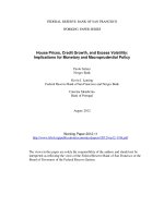
These two approaches to the arm‟s length principle are referred to as scenario for administered and as scenario
for negotiated transfer prices. The time line in Figure 1 shows the dates at which the transaction is priced
depending on the scenario. The transaction itself takes place between dates 2 and 4. In order to keep the analysis
tractable, we consider a simple model of two divisions organized by functions. The upstream division (division ,
) is responsible for the production of a product which is marketed externally by the downstream division
(division , ). The divisions are organized as profit centers, and central management pursues the interests
of the firm‟s majority shareholders.
7
The firm‟s decentralized organization can readily be motivated by ‟s
restricted computational capacity, asymmetric information between the divisions and with respect to the
conditions of the transaction, and reasons of motivating divisional managements.
Figure 1: Time line
5
See OECD (2010, § 1.5). Cf. Eden (1998, pp. 596–597) for the “affiliate bargaining approach”.
6
Considering a different status-quo point, probably set by , does not change this problem and ultimately comes to
administered transfer pricing.
7
Such an organizational structure is not uncommon in business practice. Examples are given by the Schüco International KG in
Bielefeld (Germany) or the divisions of the Whirlpool Corporation (U.S.) as described by Tang (2002, pp. 47–70).
Australian Journal of Business and Management Research Vol.1 No.6 [01-06] | September-2011
10
The production capacity being effective in the period under consideration is determined by division . It
can be interpreted as a bottleneck and may depend among others on the start-up and maintenance of production
facilities, production factors rented on a short-term basis, e.g., telecommunication lines, temporarily employed
staff, or the acquisition of licenses. markets the product. The revenue
depends on the
multiplicative inverse demand function
with denoting the production and sales
volume.
8
The exogenous constants and characterize market conditions. The choice of the sales
volume is delegated to .
9
In accordance with decentralization, is allowed to deny delivery.
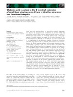
Figure 2 summarizes the relation between the divisions. The functional organization of the firm becomes evident
by the fact that all production costs accrue in . These costs consist of capacity costs , , and variable
product costs , . The parameters
denote divisional costs that are fixed in relation to capacity
and sales volume . The dotted line indicates that the production division delivers a final product and that the
marketing division actually does not have to be supplied physically.
Figure 2: Product flow and payments
Each unit of the product is valued at transfer price , whereas is a lump-sum payment from to which is
independent of the sales volume. Divisional profits
and
before compensation, taxation, and profit
distribution depend on the transfer price , the lump-sum payment , and the decisions on capacity and sales
volume . They read
(1)
and may also be called the divisions‟ gross profits from the transaction because compensation and tax payments
still have to be deducted. Note that we do not account for fixed costs since they are constants in the model and
have no influence on other parameters.
Since each of the two divisions is modeled as a taxable entity eventually having minority shareholders, we assume
that divisional managements do not seek to maximize
and
but divisional profits distributable to
shareholders, i.e., divisional profits after compensation and taxation. While tax issues are well recognized in the
transfer pricing literature, compensation issues usually are ignored unless optimal compensation plans are to be
found. The implicit assumption of this simplification is that taxation of divisional profits is the only relevant
reason for preferences on profit allocation. Here, we explicitly account for divisional compensation for three
reasons: First, correct calculation of profits distributable to shareholders makes it necessary to include
compensations. Second, it enables us to analyze whether and when compensations actually are relevant. Third, it
is actually fairly simple to include compensations if taxation and compensation are linear in divisional profits.
At first sight, the analytical derivation of divisional profits after compensation and taxation, denoted by
and
, is not trivial because taxation and compensation depend on each other. Let
denote the rate of
variable compensation of divisional management , whereas fixed compensation is included in fixed
costs. Likewise, let
denote the rate at which division ‟s profit is taxed. Then, divisional profits after
compensation and taxation are implicitly defined by the left equation of
(2)
where
is division ‟s profit after lump-sum payment but before compensation and taxation from which we
have to deduct divisional compensation and taxation. Divisional compensation is based on profits distributable to
8
The technical problem that is not defined for has no effect on the following derivations because
revenue and not the sales price is relevant.
9
The alternative specification of the sales price as ‟s decision variable has no relevance to the model. However,
the uniform choice of quantities as decision variables eases the presentation.
Australian Journal of Business and Management Research Vol.1 No.6 [01-06] | September-2011
11
shareholders and thus amounts to
. Taxable profit is defined by divisional profits after compensation, i.e.,
. The implicit expression can be solved due to the linearity of compensation and taxation. We learn that
divisional profits after compensation and taxation are proportional to divisional profits before compensation and
taxation. This is formally expressed by the right equation of (2).
While each divisional management is assumed to maximize its compensation, focuses on the sum of her
interests in divisional profits after compensation and taxation. Hence, her goal is to maximize
where
denotes ‟s interest in division . We allow for minority shareholders by assuming
. It
is important to realize that ‟s objective function is a weighted sum of divisional profits before compensation
and taxation. Consequently, is not indifferent with respect to the allocation of the firm‟s profit before
compensation and taxation to the divisions unless the weights are equal.
Returning to the relevance of compensations, we observe by (2) that compensations trivially are irrelevant if
compensation rates
and
vanish. It is also not surprising that compensations do make a difference for , if
compensation rates differ because then the relative weighting of divisional profits depends on them. However, due
to the interdependency of compensation and taxation this observation also holds true for identical positive
compensation rates whenever tax rates differ. Therefore it is justified to include divisional compensations in the
analysis.
3. NEGOTIATED TRANSFER PRICES (SCENARIO )
The analysis starts by transfer prices negotiated by the divisions prior to the transaction. Reflecting the idea that
negotiated transfer prices are considered to be arm‟s length, it is assumed that the bargaining result is not subject
to any subsequent modifications by external stakeholders. The coordinative effect of the transfer price unfolds
subsequently when division decides on the capacity and division decides on the sales volume.
10
The plot of this section is as follows: First we derive the coordinative effects and the corresponding divisional
profits induced by a two-step transfer price. Two-step transfer pricing applies because it extends the set of feasible
profits for the divisions and thereby better reflects negotiations of unrelated parties. By variation of the transfer
price, we get the set of feasible compensations and profits and thus the basis of interdivisional negotiations on the
transfer price. It can readily be observed that negotiated transfer prices are Pareto efficient. In general, however,
the divisions do not agree on the transfer price that is most preferred by central management . Hence,
may have an incentive to exert an influence on negotiations. We discuss three instruments of such influence:
Arbitration, one-step transfer prices, and revenue-based transfer prices.
3.1 Divisional decisions and equilibrium profits for given transfer price
When the divisions and negotiate the transfer price, they anticipate their optimal choices of capacity
and sales volume in reaction to the transfer price agreed upon before. Anticipation is perfect because we
assume symmetric information between the divisions. Thus, divisional decisions form a subgame-perfect
equilibrium for given transfer price.
At date 3, determines the sales volume for given two-step transfer price and given capacity in
order to maximize its compensation. Let
denote the one-step transfer price which is constant with respect to
any decision variables of the model. By (2), ‟s optimization problem reads
(3)
An immediate observation is that the scaling factor
does not bear upon ‟s
optimal sales volume. In other words, the maximization of divisional profit before compensation and taxation
corresponds to the maximization of divisional profit after compensation and taxation and thus of divisional
compensation. By (1), the additive lump-sum payment has no coordinative effect either. Also note that (3) is
based on the assumption that agrees to deliver quantity . Hence, we require the transfer price not to fall short
of the variable unit costs . The result of ‟s optimization is referred to as
.
Anticipating the sales volume
, maximizes its compensation with respect to capacity, i.e.,
10
In contrast to Halperin and Srinidhi (1991), divisions do not negotiate decision variables which have been
delegated to one of them. Consequently, the transfer price preserves its coordination function.
Australian Journal of Business and Management Research Vol.1 No.6 [01-06] | September-2011
12
and obtains equilibrium capacity
. Like , actually maximizes its profit before lump-sum payment,
compensation, and taxation. Lemma 1 computes the equilibrium in divisional decisions.
Lemma 1. Under negotiated transfer prices, the equilibrium capacity
and sales volume
for
given transfer price
are
For
, the equilibrium in Lemma 1 is governed by the marketing division because the equilibrium
quantity results from equating marginal revenue to marginal costs based on ‟s profit, i.e.,
By contrast, ‟s optimization can be reduced to the question whether the transfer price
covers total marginal
costs. These costs do not only consist of for setting up the capacity but also of variable unit costs resulting
from capacity utilization since optimally has no idle capacity. In case the transfer price
does not cover
total marginal costs , chooses zero capacity in order to prevent a loss from the transaction. Otherwise,
maximizes its divisional profit by setting up the maximal fully utilized capacity.
Plugging these decisions in the profit functions (1) yields equilibrium divisional profits before compensation and
taxation, i.e.,
and
. For notational convenience we refer to them as
and
. Likewise, the corresponding profits after compensation and taxation are denoted by
and
. The following corollary evaluates divisional profits before compensation and
taxation.
11
Corollary 1. Under negotiated transfer prices, equilibrium divisional profits
and
before
compensation and taxation are given by
These profit functions exhibit strictly quasi-concave graphs on and thus have unique maximizers. We
refer to these maximizers as
and
and easily compute
. Note that the
interval
consists of Pareto-efficient one-step transfer prices
.
3.2 Negotiated two-step transfer price
Having determined the divisional profits resulting from a given transfer price, we are now able to analyze
interdivisional negotiations on the transfer price itself. In accordance with the divisions maximizing their
respective compensations when deciding on the capacity and the sales volume, we start on the premise that the
divisions negotiate on the basis of compensations. The first step is to determine feasible pairs of compensation.
Then we derive the negotiated transfer price according to axiomatic bargaining theory.
12
The set
(4)
contains all pairs of divisional compensations that are feasible by variation of the two-step transfer price
.
13
As depicted by Figure 3, it is instructive to construct this set in two steps:
14
First, set the lump sum to zero and
choose a transfer price
, i.e., pick one pair of compensations from the set
11
Corollary 1 results from direct evaluation of the functions
and
. The proof is omitted.
12
See, e.g., Rosenmüller (2000, ch. 8) and Myerson (1997, ch. 8) for axiomatic bargaining theory.
13
For simplification, we do not account for free disposal of compensations or divisional profits.
14
The parameters to generate Figure 3 are , , and
.
Australian Journal of Business and Management Research Vol.1 No.6 [01-06] | September-2011
13
. In Figure 3 this is done for transfer prices
(lower parallel) and
(upper parallel). Second,
starting from this point vary lump sum to shift compensation between and . (4) collects all pairs of
compensations resulting from applying this procedure to all transfer prices
.
Figure 3: Divisional compensations in scenario
Although the lump sum is able to shift compensation between divisions at a constant rate, it generally does not
allow a symmetric transfer. This is because the lump sum is based on profits before compensation and taxation and
thus is still subject to compensation and taxation. The transfer rate of compensation is easy to calculate: We know
by (2) that one unit of the lump sum increases ‟s compensation by
and
decreases ‟s compensation by
. This yields a rate of
which determines the negative slopes of the parallels in Figure 3.
In order to derive a specific bargaining solution, we assume that the divisions cooperatively agree on a proper
bargaining solution, i.e., a feasible bargaining solution satisfying the basic axioms of individual rationality, Pareto
efficiency, covariance with permutations, and covariance with positive affine transformations of utility. Note that
the well-known Nash bargaining solutions satisfy this minimal set of properties. By virtue of the two-step transfer
price, these axioms suffice to determine a unique bargaining solution:
Proposition 1. Under negotiated two-step transfer pricing, the divisions agree on transfer price
with
and
. The corresponding divisional profits before compensation and
taxation amount to
.
To understand why Proposition 1 holds, refer to Figure 3 which shows that the lump sum transfers compensation
between the divisions at rate
. Thus, Pareto efficiency calls for a transfer price
maximizing
By (2), this is equivalent to the maximization of the equally weighted sum of divisional profits before
compensation and taxation, i.e.,
, with respect to
. Referring to Corollary 1, this
maximizer turns out to equal
and induces the upper parallel in Figure 3. We finally observe that
compensations or taxes do not play a role for negotiations. This reflects the axiom of covariation with positive
affine transformations of utility, i.e., the bargaining solution covaries with the scaling of divisional profits.
There is fairness interpretation of the negotiated lump sum. The status-quo point zero restricts feasible values of
the lump sum because no agreement shall be worse for any division than disagreement. We therefore exclude
Australian Journal of Business and Management Research Vol.1 No.6 [01-06] | September-2011
14
individually irrational lump sums which are indicated by dashed lines in Figure 3. Hence, the negotiated lump sum
is an element of the interval
.
picks the center of this interval inducing equal divisional
profits before compensation and taxation. However, this does not imply equal compensations among the
divisions. Rather, as indicated in Figure 3 by dotted lines, compensations relative to maximal individually rational
and Pareto-efficient compensations are equal.
15
Before we analyze ‟s incentives and possibilities to exert an influence on interdivisional negotiations, we
stress that the negotiated transfer price given in Proposition 1 is Pareto efficient. For further illustration of this
point, let the divisions be subject to different tax jurisdictions of which we assume that each of the two involved
tax authorities is interested in high tax yields and therefore in high profits after compensation of the corresponding
division. Analogously to (2), it can be checked easily that divisional profits after compensation, denoted by
,
are also proportional to divisional profits before compensation, more precisely
. Hence,
any deviation from the negotiated transfer price
yields smaller tax returns for at least one of the two tax
authorities. In like manner, other stakeholders such as minority shareholders can easily be included in the analysis
by an appropriate specification of the weights on divisional gross profits.
3.3 Incentives and possibilities for to manipulate negotiations
From the perspective of central management, the negotiated transfer price
is not the most favorable
transfer price. would rather maximize the sum of her interests, i.e.,
.
Figure 4 depicts the situation in terms of divisional profits before compensation and taxation.
16
The negotiated
transfer price
yields point A whereas the most favorable bargaining result from ‟s perspective is
given by point B if puts higher a weight on profits in division than in . This is equivalent to weights
satisfying
. For the opposite weighting, most prefers point C. For notational
convenience we introduce
as ‟s weight of division ‟s, , profit before compensation and taxation.
Figure 4: Divisional profits before compensation and taxation in scenario
In the following, we analyze three instruments for to exert an influence on the divisions‟ negotiations to her
advantage, namely 1) arbitration, 2) one-step transfer pricing, and 3) revenue-based transfer pricing. The analysis
concentrates on their profit consequences for a given parameter setting. Since is assumed to be imperfectly
informed on the parameter setting she would have to form expectations on the instruments‟ consequences in order
to deploy them optimally. The following results are the basis of such optimal choice under imperfect information.
15
This particular idea of fairness is characteristic of the Kalai-Smorodinsky solution.
16
The graphs of Figure 4 are based on the parameters and .
Australian Journal of Business and Management Research Vol.1 No.6 [01-06] | September-2011
15
Arbitration
Proposition 1 is based on the status-quo point zero reflecting that the divisions have no outside options for the
specific transaction at hand. More importantly, it reflects the absence of an arbitrator and thus the idea of a market
solution. By contrast, in an integrated firm it is not exceptional that acts as a mediator or arbitrator in transfer
pricing disputes between the divisions. One way of arbitration is to stipulate a fall-back transfer price for the case
that the divisions fail to find an agreement on the transfer price. For plausibility we assume that this fall-back
transfer price only applies in case the divisions actually engage in internal trade. At first sight, such arbitration
seems irrelevant for the model since the divisions always come to an agreement. However, a fall-back transfer
price may change the status-quo point of the bargaining problem so that the set of feasible, individually rational,
and Pareto-efficient divisional profits change. In Figure 4, this situation is depicted for a fall-back transfer price
shifting the status-quo point to point D. Each bargaining solution then yields point E as the bargaining result. As
indicated by the small dotted square, this point grants both divisions the same surplus before compensation and
taxation in relation to the status-quo point D. Proposition 2 gives the general result.
Proposition 2. Under negotiated two-step transfer pricing and fall-back transfer price
, the divisions
agree on transfer price
with
if
. The corresponding divisional profits before compensation and taxation are
and
. Otherwise the fall-back transfer price has no
effect.
The status-quo point of the bargaining problem only changes if both divisions do not loose from internal trade at
the fall-back transfer price because each of the divisions may avoid internal trade and thereby incur zero profit.
Consequently, arbitration may be ineffective for inadequate fall-back transfer prices and Proposition 1 applies.
For effective arbitration, it does not surprise that only the lump sum reacts to the shift of the status-quo point. The
magnitude of this reaction is captured by the second term of the sum determining
. Consequently, whenever
puts a higher (resp. lower) weight on than on in terms of profits before compensation and taxation,
she benefits from a shift of the status-quo point which advantages division (resp. ). Given the situation of
Figure 4, benefits from bargaining solution E in comparison to A, iff the parameters satisfy
.
In fact, shifting the status-quo point by means of a fall-back transfer price is an effective instrument to manipulate
negotiations because it is capable of shifting profits in both directions and most notably of any magnitude. The
downside is that runs the risk that the fall-back transfer is ineffective. In expectation, however, is always
able to gain from arbitration.
One-step transfer prices
In spite of greater flexibility, two-step transfer pricing is not common in business practice. According to Tang
(1993, 71), only one percent of 143 firms employ two-step transfer prices. Hence, a restriction of interdivisional
negotiations to a one-step scheme presumably does not cause mistrust among external stakeholders. One-step
transfer pricing brings about a different bargaining problem because both coordination and profit allocation have
to be accomplished by the same parameter, namely the unit transfer price .
Feasible divisional profits under one-step transfer pricing are described by the set
of which Figure 4 exhibits a typical graph. Apparently, it is not possible to transfer profits or compensations
between the divisions at a constant rate as under two-step transfer pricing. Consequently, there is more than one
proper bargaining solution. We focus on the Nash bargaining solution:
Proposition 3. Under negotiated transfer pricing, the one-step transfer price of the Nash bargaining solution is
and induces equilibrium divisional profits
Australian Journal of Business and Management Research Vol.1 No.6 [01-06] | September-2011
16
The Nash bargaining solution chooses the transfer price that maximizes the product of divisional profits.
17
It
corresponds to point F in Figure 4. The relations
and
say
that, given the Nash bargaining solution, one-step negotiated transfer pricing favors the downstream division.
Referring to Figure 4, this is equivalent to the fact that the Nash solution F always lies to the left of and above
point A. Hence, prefers one-step to two-step transfer pricing iff she is characterized by a sufficiently high
weight on ‟s profit. Proposition 4 provides a precise result for this idea.
Proposition 4. Assuming that the divisions agree on the Nash bargaining solution, central management prefers
one-step to two-step transfer prices iff she puts a sufficiently higher weight on downstream relative to upstream
gross profits. The precise condition is
where the constant is defined as
The approach to determine the critical relative weighting is straight forward: It is the slope of the line
connecting points A and F in Figure 4 in the
plane. Put differently, if had relative weighting
, she would be indifferent between one-step and two-step transfer pricing. Any higher (resp. lower) relative
weighting causes her to prefer one-step (resp. two-step) prices. The critical value also applies for other
stakeholders. For example, the tax authority with jurisdiction over the upstream division has weights
and
and would never benefit from switching to one-step transfer pricing due to
.
Revenue-based transfer prices
According to Proposition 4, it is not worthwhile for to switch from two-step to one-step transfer pricing if her
weight on downstream profits is relatively low because one-step transfer pricing benefits the downstream
division. However, this result depends on the transfer pricing scheme. In fact, may consider to base the
scheme on revenue so that the downstream division pays the price
per sales unit. Negotiations
then concentrate on parameter
and thus specify a rule of revenue sharing. This scheme can readily be
matched with the resale price method known from international taxation. Likewise, defining the transfer price as
, as we have done so far, can be linked to the comparable uncontrolled price or the cost plus method. The
resale price method is considered particularly suitable for transactions of functionally organized divisions with the
downstream division providing little contributions to the manufacturing of the final product.
18
Therefore, the
application of scheme in our context presumably would not seem odd to external stakeholders. In the following,
we refer to
as scheme and to
as scheme .
A change in the transfer pricing scheme has a significant impact on coordination and thus on divisional profits
since the transfer price under scheme depends on the sales volume which is a delegated decision. As an analog
of Lemma 1 and Corollary 1, we get the following equilibrium divisional decisions and profits.
Lemma 2. Under negotiated transfer pricing, the equilibrium capacity
and sales volume
for
given transfer price
are
Equilibrium divisional profits before compensation and taxation read
In contrast to scheme , is able to influence the transfer price under scheme : may raise the transfer
price by making capacity scarce, i.e., by choosing such small a capacity that is effectively constrained in
setting the sales volume. Thereby the share
of marginal revenue as to capacity accrues to . Since revenue
maximization by implies vanishing marginal revenue, the optimal capacity is scarce from ‟s perspective.
19
17
Haake and Martini (2011) provide a fairness interpretation of the Nash bargaining solution.
18
Cf., e.g., OECD (2010, ch. 2),U.S. Internal Revenue Code Regulations § 1.482-3, or Eden (1998, pp. 36–45) for
the methods.
19
Note that the fact that ‟s optimal capacity choice constrains ‟s revenue maximization is not an artifact of
themultiplicative demand function.
Australian Journal of Business and Management Research Vol.1 No.6 [01-06] | September-2011
17
The optimal restriction of the sales volume is reached when partial marginal revenue equals total marginal costs of
capacity amounting to . Hence, the equilibrium capacity may be calculated as
which implies an equilibrium capacity that strictly increases in the sharing parameter
. Consequently, it is
primarily the production division which induces equilibrium decisions.
Referring to Figure 4, we observe that the set of feasible and Pareto-efficient divisional profits for two-step
transfer prices is the same under both schemes, i.e.,
holds where
denotes the negotiated sharing parameter. We easily verify that the negotiated revenue sharing
parameter equals
and induces the same aggregate profit before compensation and taxation as scheme :
An important conclusion hereof is that negotiations over two-step transfer prices do not depend on the scheme as
far as divisional profits are concerned. Indeed, there is no scheme at all providing a higher sum of divisional
profits before compensation and taxation than schemes and because the induced divisional decisions
maximize firm-wide profit before compensation and taxation. Note that these results concerning the equivalence
and optimality of two-step schemes are peculiar to the model.
20
There clearly is no point for in switching from one two-step scheme to another. Yet, Figure 4 shows that
may benefit from switching to one-step revenue-based transfer pricing: In comparison with two-step transfer
pricing, represented by point A, the Nash solution for one-step revenue-based transfer pricing, represented by
point G, favors the upstream division. The following proposition computes the Nash bargaining solution and
proves by expression (5) that this observation can be generalized.
21
Proposition 5. Under negotiated transfer pricing, the one-step revenue-based transfer price of the Nash
bargaining solution is
and induces equilibrium divisional profits
(5)
Similar to the reasoning of Proposition 4, we are able to determine a threshold of ‟s relative weighting of
divisional profits such that she finds it profitable to confine negotiations to one-step transfer prices based on
scheme instead ofletting the divisions negotiate on two-step transfer prices.
22
Proposition 6. Assuming that the divisions agree on the Nash bargaining solution, central management prefers
one-step revenue-based to two-step transfer pricing iff she puts a sufficiently higher weight on upstream relative
to downstream gross profits. The precise condition is
where the constant is defined as
Figure 5 combines the results of Propositions 4 and 6. It focuses on ‟s preference over the schemes depending
on her relative weighting of divisional profits. Nevertheless, it can be directly applied to any other stakeholder.
Note that the threshold values and only depend on the demand parameter . This simplifies ‟s
decision problem. Simplification is most pronounced if ‟s weighting lies in the same of the intervals ,
20
See Haake and Martini (2011) for different effects in a model with divisional investments.
21
The proof of Proposition 5 is omitted because it is an analog of the proof of Proposition 3.
22
The proof of Proposition 6 is omitted because it is an analog of the proof of Proposition 4.
Australian Journal of Business and Management Research Vol.1 No.6 [01-06] | September-2011
18
, or for all realizations of the unknown parameter : Then the optimal scheme can be inferred
directly from that interval.
Figure 5: ’s preferred negotiated transfer pricing scheme
4. ADMINISTERED TRANSFER PRICES (SCENARIO )
Under administered transfer prices, the setting changes with respect to two important aspects. First, it is who
sets the transfer price and the divisions do not negotiate. Consequently, and external stakeholders cannot
directly refer to the ‟true„ arm‟s length price given by the negotiated transfer price in Proposition 1. Due to the
shortage of identical uncontrolled transactions or data thereof arm‟s length pricing thus becomes a matter of
discretion. Second, typically files after the transaction so that we concentrate on date 5 when analyzing the
transfer pricing choice.
We analyze two different range formulations with respect to the discretion inherent to the arm‟s length principle
and the corresponding regulations. Both formulations demonstrate that administered transfer prices risk to be
Pareto inefficient from an ex-ante perspective. Such an inefficiency is unfavorable for any stakeholder and we
discuss ways of preventing it. For both approaches, we assume that arm‟s length prices are one-step which, as
mentioned before, reflects business practice.
4.1 Transfer prices based on a single scheme (scenario
)
Under administered transfer prices, documents the conformity with the arm‟s length principle on the basis of
data on comparable transactions. As there are typically no perfect comparables for the considered transaction only
a range of arm‟s length prices might be derived.
23
We reflect this fact by parameter ranges
and
, respectively. Their endpoints
and
with
represent the minimal and maximal
parameter values which can be justified by to relevant stakeholders under scheme . The following
results are general in that they do not depend on further consistency conditions imposed on the ranges. Following
Smith (2002a), for instance, one might require that the ranges are centered around the one-step equivalent of the
negotiated transfer price given by Proposition 1. By contrast, Martini (2008) illustrates the range of arm‟s length
prices in a model which explicitly incorporates information asymmetry by intervals containing the expected rather
than the actual negotiated transfer price. Moreover, we do not explicitly account for ex-ante discretion, i.e., for an
influence of prior investment decisions on the arm‟s length ranges because the model concentrates on the
economics of the transaction for given investment effects.
24
Note further that we model external arm‟s length
comparisons which means that comparables are not traded with the firm under consideration.
25
For the scenario
, we assume that applies a single scheme for the derivation of an arm‟s length transfer
price. This is in line with regulations of international taxation which typically do not require to apply more than
one method.
26
Moreover, the actual choice of the scheme is exogenous to the analysis which can be justified by
the circumstance that the decision on the scheme is taken less frequently than the one on the value of the transfer
price. This may be due to several reasons, some important of which are implementation costs, the principle to
adhere to a once chosen accounting policy, the existence of a recommended method for tax purposes, the existence
of an intra-firm guideline or an advance pricing agreement, or the fact that a change of the scheme may be hard to
justify toward external stakeholders, especially toward tax authorities. Moreover, the availability and quality of
data on comparable transactions may call for one of the schemes.
Given these assumptions, may choose either any transfer price
for scheme or
for scheme . On the basis of the analysis of negotiated transfer prices, it is straight forward to
state the set of feasible divisional profits as
23
Cf. OECD (2010, §§ 3.55–3.62) or U.S. Internal Revenue Code Regulations § 1.482-1(e)(1) for the “arm‟s
length range”.
24
See Martini (2008) or Smith (2002a) for endogenous investment decisions.
25
See Halperin and Srinidhi (1991) for a model with internal comparisons.
26
See, e.g., OECD (2010, § 2.11) or U.S. Internal Revenue Code Regulations 1.482-1(c)(1) and 1.482-1(e)(2)(i).
Australian Journal of Business and Management Research Vol.1 No.6 [01-06] | September-2011
19
if we assume that both divisions anticipate the transfer pricing parameter
, . Hence, feasible divisional
profits under administered transfer prices are a subset of feasible divisional profits under negotiated transfer
prices. Figure 6 provides an example.
27
The dotted parts of the curves indicate feasible profits under negotiated
transfer pricing.
Figure 6: Divisional profits in scenario
‟s chooses the transfer price when divisional decisions are taken. At this point, the transfer price exclusively
serves profit allocation, coordinative effects are foregone. ‟s transfer pricing choice therefore is a corner
solution: She selects parameter
, , according to
(6)
in order to maximize or minimize the transfer payment. In the top case, for instance, chooses the smallest
arm‟s length price because she is more interested in ‟s profit than in ‟s. In the following, we disregard the
case of being indifferent.
It is important to realize that this behavior is only optimal from an ex-post perspective because it ignores effects on
coordination. In other words,
generally does not maximize
. It is even possible that a
combination of divisional profits occurs that is Pareto inefficient from an ex-ante perspective. Figure 6 depicts an
instructive example for scheme . Suppose that puts more emphasis on ‟s profit than on ‟s and thus
chooses the low transfer price parameter
. From an ex-ante perspective, the induced profits are inefficient from
any stakeholder‟s perspective since there are parameters from the arm‟s length range implying higher a profit for
at least one of the divisions while keeping the other division at least at the initial profit level. Preliminary to
Proposition 7 which states all situations of such inefficiency, we introduce the counterparts of the maximizers
and
for scheme :
Proposition 7. Under administered transfer prices based on a single scheme, divisional profits are Pareto
inefficient from an ex-ante perspective, iff
27
Figure 6 is based on the parameters , ,
,
,
, and
.
Australian Journal of Business and Management Research Vol.1 No.6 [01-06] | September-2011
20
1.
and
, or
and
holds for scheme , or
2.
and
holds for scheme .
The proposition essentially says that, from an ex-ante perspective, chooses an inefficient transfer price if the
arm‟s length range contains inefficient transfer prices lying on the ‟wrong„ side of the range. Interestingly, scheme
is more robust than scheme in that inefficiency may only occur for
because for scheme there are
no large inefficient transfer price parameters. Note that the problem of ex-ante inefficiency occurs although the
transfer price choice at date 5 is optimal and thus sequentially rational. An advance commitment of might
prove an effective remedy against this dilemma of sequential rationality, and , as well as all other
stakeholders, have a vital interest to make use of it.
There are at least two instruments of such commitment. The most formal devices are advance pricing agreements
and internal transfer pricing guidelines. Observe that the presented interpretation of these instruments as devices
of preventing to ignore coordinative effects on divisional profits is innovative. Commonly they are used to
reduce uncertainties, costs, and conflicts in the course of the approval of transfer prices.
28
Extending the time
horizon of the model, one may also derive a commitment effect from ‟s current transfer pricing choice on later
periods if arm‟s length ranges depend on the history of ‟s past choices. In this context, Ernst & Young (2008,
14) find that changes in transfer prices are perceived to be second most likely to trigger a tax audit. Hence, ‟s
initial choice limits her future transfer price choices implying a less myopic pricing behavior. One would also
expect high demands on the documentation of arm‟s length transfer pricing to support the binding effect of past
pricing choices. This perspective challenges the idea that firms suffer from higher documentation requirements
which restrict their ability to evade taxes and profit distributions to minority shareholders.
In addition to inefficient transfer prices, there may be situations of an inefficient scheme so that any stakeholder ex
ante prefers one scheme to the other. Proposition 8 states that such type of inefficiency might arise independently
of ‟s weighting of divisional profits and that both schemes are candidates for inefficiency.
Proposition 8. Under administered transfer prices based on a single scheme, there are values of parameters
and
for
and
such that divisional profits for one scheme are Pareto inefficient from
an ex-ante perspective in comparison to divisional profits for the other scheme. Such parameters satisfy
,
, or both.
Figure 6 also provides an example of an inefficient scheme since for
scheme yields higher profits for
both divisions than scheme . would try to avoid such type of inefficiency by an appropriate initial choice of
the scheme. The condition given at the end of the proposition says that at least one of the pricing choices
or
has to be Pareto inefficient within its scheme for unrestricted parameter choice. At first sight, it is puzzling
that inefficiency within a scheme plays a role here. However, it is a special feature of this model that efficiency of
a pricing choice within one scheme with no restriction on feasible transfer prices is equivalent to the efficiency of
the scheme.
Taking up the topic of asymmetric information, one might ask how should become aware of the described
inefficiencies under asymmetric information. We give two answers. First, obviously may always form
expectations based on her knowledge of the transaction‟s conditions. Second, might have the divisions report
whether they support an increase or a decrease in the transfer price or a change of the scheme: Only for
Pareto-inefficient transfer prices their reports are unanimous giving the possibility to anticipate inefficient
pricing choices.
4.2 Crosschecking (scenario
)
In scenario
, each scheme is considered sufficient so that restricts herself to one of the schemes when
choosing an arm‟s length price. However, such an approach is extreme bearing in mind that data on comparables
typically depend on the scheme. An alternative way to cope with the fuzziness of arm‟s length pricing is to include
data for more than one scheme in order to find transfer prices that are consistent with several schemes. By doing
so, crosschecks an arm‟s length price based on one scheme and preempts potential objections by other
stakeholders on the basis of the other scheme.
29
Note that scenarios
and
do not necessarily call for legal
28
Cf. OECD (2010, §§ 4.123–4.138) for advance pricing agreements and their advantages.
29
See OECD (2010, §§ 2.11, 3.58) for the OECD guidelines on crosschecking. In U.S. tax law, crosschecking is
implicit to the best method rule and the arm‟s length range. See U.S. Internal Revenue Code Regulations §§
1.482-1(c), 1.482-1(e)(2)(i), 1.6662-6(d). It can also be interpreted as an unspecified method, see U.S. Internal
Revenue Code Regulations §§ 1.482-3(e), 1.482-4(d).
Australian Journal of Business and Management Research Vol.1 No.6 [01-06] | September-2011
21
codification or have to be carried out explicitly. They rather constitute different ways of modeling the discretion
and complexity typically associated with the evaluation of transfer prices and the procedures thereof.
There are several approaches to combine both schemes. One possibility is that arm‟s length prices have to be
accepted under both schemes. Thus arm‟s length prices are given by the intersection of the intervals
and
. A drawback of this approach is that it is difficult to interpret an empty intersection. There is
another, more robust approach to „average‟ the ranges: The endpoints of the aggregate arm‟s length range
are defined as convex combinations of the left respectively the right endpoints of the individual ranges:
The weight can readily be interpreted as a measure of scheme ‟s adequacy relative to scheme .
Scenario
uses to model transfer prices based on a single scheme. An important observation is that
crosschecking makes the issue of the employed scheme obsolete since always both schemes are considered due to
the aggregation. Hence, assertions on preferences on the schemes like Propositions 4, 6, or 8 cannot be made
under the crosschecking scenario
.
Lemma 3 states the equilibrium decisions in scenario
which are different from those in scenarios and
. In
order to simplify the presentation, we make use of the parameter
representing a standardized transfer
price defined by
Thus,
gives the position of an accepted transfer price within the arm‟s length range
. For
example,
(resp.
) corresponds to transfer price
(resp.
).
Lemma 3. Under administered transfer pricing with crosschecking, the equilibrium capacity
and
sales volume
for standardized transfer price
are given by
where
, , and
, , are defined as
For sufficiently high arm‟s length prices under scheme , and thereby a high value of
, the equilibrium is
comparable to that of scheme in the scenarios and
: The sales volume is optimal from ‟s perspective,
here
, and installs the corresponding capacity. Otherwise, i.e., for sufficiently small arm‟s length
prices under scheme , has an incentive to make capacity scarce, here
, in order to benefit from an
increase of the transfer price whereas just sells up to ‟s capacity.
Figure 7 depicts the equilibrium profits depending on the standardized transfer price
.
30
The notations
are used to denote the set of ex-ante feasible divisional profits more conveniently. Keeping in mind that
chooses, in analogy to expression (6) in scenario
, extreme transfer prices
according to
it is intuitive that the dilemma of ex-ante inefficiency of ex-post efficient transfer prices may occur under
crosschecking, too. We capture this result by the following corollary.
30
The parameter setting of Figure 7 is , ,
,
,
,
, and .
Australian Journal of Business and Management Research Vol.1 No.6 [01-06] | September-2011
22
Figure 7. Divisional profits in scenario
Corollary 2. Under administered transfer pricing with crosschecking, there are parameter settings for
and
so that divisional profits are Pareto inefficient from an ex-ante perspective.
Figure 7 does not only serve as the proof and as an illustration of Corollary 2 but also allows to make the
interesting observation that crosschecking itself might induce ex-ante inefficiency of the chosen transfer price.
This observation holds because the figure is based on individual arm‟s length ranges which do not contain ex-ante
inefficient transfer prices so that the observed inefficiencies stem from the combination of the schemes rather than
from the individual schemes.
For crosschecked schemes, cannot evade the dilemma of sequential rationality by committing herself to one
of the schemes in advance. Yet, in general the same commitment devices as mentioned for scenario
can be
applied. Since crosschecking is more involved than transfer pricing based on a single scheme, the corresponding
terms of an advance pricing agreement or an intra-firm transfer pricing guideline have to be more elaborate.
5. RESULTS AND DISCUSSION
This paper examines the common practice of a single set of books implying that one transfer price couples the two
functions of coordination and profit allocation. The analysis focuses on efficiency and shows different results
depending on the approach to the arm‟s length principle.
Administered transfer prices maximize the firm‟s profit net of compensations, taxes, and minority profit shares.
Yet, as administered transfer prices typically refer to past transactions, they ignore effects on divisional decisions.
By virtue of the profit-center organization, these decisions are egoistic and thus do not take firm-wide effects into
consideration. They are even not influenced by the division‟s own compensation or taxes although they are based
on divisional profits distributable to shareholders. The most salient consequence is the risk of divisional profits
that are Pareto inefficient from an ex-ante perspective which are unfavorable for any stakeholder. The risk exists
for arm‟s length prices derived from a single transfer pricing scheme and as well as from crosschecked schemes.
Consequently, ex ante, the firm itself may have an incentive to restrict ex-post discretion over arm‟s length prices
and therefore initiate an advance pricing agreement for tax purposes. A restrictive treatment of changes in the
firm‟s accounting policy supported by high demands on the transfer pricing documentation has a similar effect.
Other contributions assume that central management chooses an arm‟s length price in anticipation of its effect on
both coordination and profit allocation.
31
This paper complements those approaches on the one hand by stressing
that this necessitates a commitment of central management not to be sequentially rational, and on the other hand
by identifying instruments of such commitment.
31
Cf. Baldenius, Melumad, and Reichelstein (2004), Narayanan and Smith (2000), and Schjelderup and Sorgard
(1997).
Australian Journal of Business and Management Research Vol.1 No.6 [01-06] | September-2011
23
In contrast to administered transfer prices, negotiated transfer pricing produce Pareto-efficient divisional profits
for all stakeholders. Moreover, interdivisional negotiations are compelling as they seem to be a perfect
operationalization of the arm‟s length principle. However, we show that common transfer pricing practices
deployed by majority shareholders may influence the bargaining result to their advantage. For example, switching
to a one-step scheme shifts profits to the upstream division whereas a one-step revenue-based transfer price favors
the downstream division.
Both negotiated and administered transfer pricing are extreme. Administered transfer pricing ignores that
incorporated profit centers often come to contractual agreements ruling the transactions between them. On the
other hand, external stakeholders may be skeptical whether interdivisional negotiations actually are at arm‟s
length. A descriptive way to combine the scenarios is to let the divisions negotiate the contractual terms of the
transaction including the transfer price in the first place. At the end of the period, central management documents
that the agreements actually are at arm‟s length by crosschecking against arm‟s length ranges based on data on
comparables. Correction of negotiated prices would only be justified if they are outside the ranges. In this hybrid
scenario, which might be called negotiated transfer pricing with crosschecking, the major influence on the transfer
price is exerted by the divisions. Hence, negotiated transfer prices are Pareto-efficient given the limits of the arm‟s
length range.
APPENDIX
Proof of Lemma 1
‟s optimal sales volume for
is
. Thus maximizes
(7)
with respect to . Note that does not benefit from any excess capacity so that the bottom case of (7) can
be ignored. Assuming to choose
in case of indifference, i.e.,
, equilibrium
capacity is
which entails the equilibrium sales volume
. In case
,
denies delivery and does not set up any capacity.
Proof of Proposition 1
Since the bargaining solution covaries with positive affine transformations we may focus on divisional profits
before compensation and taxation when deriving the bargaining solution. Note that, before compensation and
taxation, the lump sum arbitrarily transfers profit between the divisions at rate 1.
Pareto efficiency calls for the transfer price
. On the basis of Corollary 1,
we easily verify that
maximizes the sum of divisional profits before compensation and taxation.
Symmetry of the bargaining solution and zero as the status-quo point imply that divisional profits before
compensation and taxation have to be equal. Again by Corollary 1, the negotiated lump sum
therefore amounts
to half of the aggregate surplus
. Divisional profits result from
straight evaluations.
Proof of Proposition 2
The status-quo point of the bargaining problem only changes if both divisions do not loose from internal trade at
the fall-back transfer price because each of the divisions may avoid internal trade and thereby incur zero profit. In
the following, we therefore require
.
Refer to the proof of Proposition 1 for preliminary remarks, the derivation of the negotiated transfer price
, and the approach to determine the negotiated lump sum. Here, the aggregate surplus with
respect to the status-quo point amounts to
which can easily be simplified to
. By symmetry, this surplus has to
be equally allocated to the divisions. Taking the status-quo point into consideration this leads to
Australian Journal of Business and Management Research Vol.1 No.6 [01-06] | September-2011
24
Divisional profits result from straight evaluations.
Proof of Proposition 3
The Nash bargaining solution,
, maximizes the product of divisional
surpluses. It is straight forward to calculate it on the basis of Corollary 1. This also applies to the calculations to
obtain relations the
,
, and
.
Proof of Proposition 4
‟s preference over divisional profits is reflected by the sum of her interests,
. The
level curves of this preference function are lines in the
plane with negative slope
. For
divisional profits of the Nash bargaining solution under two-step and one-step transfer pricing exhibit identical
sums of interests. By Propositions 1 and 3, it is easily checked that this condition is equivalent to
(8)
Since holds by assumption, the left-hand side of (8) takes values between and
. One-step transfer pricing induces a higher sum of interests for than two-step
transfer pricing, iff exceeds the critical value of the left-hand side of (8) because
and
holds by Proposition 3.
Proof of Lemma 2
For scheme , maximizes revenues entailing that the optimal sales volume is only bounded by capacity or
‟s agreement to deliver. The optimal sales volume therefore is
where it has
to be assumed that chooses quantity
in case of indifference, i.e., for
. The capacity
maximizes
and induces equilibrium sales volume
. Equilibrium profits result from direct
evaluations of the functions
and
.
Proof of Proposition 7
Refer to Corollary 1 and Lemma 2 for the definitions of
, , . Note that
as the set of feasible profits under scheme is described by a strictly concave
graph in the
plane with
and
. Divisional profits are continuous in
. Otherwise they are zero. For unrestricted
parameter
, Pareto-inefficient transfer prices fall into intervals
and
. In the light of the
definition of
given by (6), the assertion with respect to scheme follows easily. For scheme we would
proceed in a similar manner.
Proof of Proposition 8
Refer to Corollary 1 and Lemma 2 for the definitions of
,
,
. The properties of
,
, are mentioned in the proof of Proposition 7. Feasible profits under scheme , i.e.,
Australian Journal of Business and Management Research Vol.1 No.6 [01-06] | September-2011
25
, are described by a strictly concave graph in the
plane with
and
. Divisional profits are continuous in
.
For unrestricted parameter
, Pareto-inefficient parameters for scheme fall into the interval
.
Additionally, the graphs of feasible profits intersect for the maximal Pareto-efficient parameter
and the
minimal Pareto-efficient parameter
:
. Due to these
properties, any pair of divisional profits under scheme with
is Pareto-efficient in comparison
to any pair of divisional profits under scheme with
. Such settings are excluded in the proposition.
Examples of inefficiency are easily found for any mentioned setting.
Proof of Lemma 3
We start by assuming
. Considering that the transfer price is equivalent to
, ‟s profit function reads
.
Since
holds, is motivated to deliver and maximizes
for . The solution is
. Thus, chooses the capacity maximizing
for
. Since excessive capacity cannot be optimal for ,
we have
and thereby
in equilibrium. For
the maximizer of
is
, otherwise wants to expandcapacity unboundedly.
and
follow immediately.
In case
holds, we additionally have to account for ‟s agreement to deliver when determining the
optimal sales volume. This yields a maximal sales volume of
implying
. Since
holds, again installs capacity
.
REFERENCES
1. Balachandran, K. R., & Li, S H. (1996). Effects of differential tax rates on transfer pricing. Journal of
Accounting, Auditing and Finance, 11(2), 183–196.
2. Baldenius, T., Melumad, N. D., & Reichelstein, S. (2004). Integrating managerial and tax objectives in
transfer pricing. The Accounting Review, 79(3), 591–615.
3. Eden, L. (1998). Taxing multinationals: Transfer pricing and corporate income taxation in North
America. Toronto, Buffalo: University of Toronto Press.
4. Elitzur, R., & Mintz, J. (1996). Transfer pricing rules and corporate tax competition. Journal of Public
Economics, 60(3), 401–422.
5. Ernst & Young (2003). Transfer pricing 2003 global survey. EYGM Limited. Available from
/>rt_2003.pdf/$FILE/Transfer+Pricing+Survey+Report_2003.pdf.
6. Ernst & Young. (2008). Global transfer pricing survey 2007–2008. EYGM Limited. Available from
www.ey.com/Publication/vwLUAssets/Precision_under_pressure/$FILE/Precision_under_pressure.pdf
7. Haake, C J., & Martini, J. T. (2011). Negotiating transfer prices. Working paper. Available from
8. Halperin, R., & Srinidhi, B. (1987). The effects of the U.S. income tax regulations‟ transfer pricing rules
on allocative efficiency. The Accounting Review, 62(4), 686–706.
9. Halperin, R., & Srinidhi, B. (1991). U.S. income tax transfer-pricing rules and resource allocation: The
case of decentralized multinational firms. The Accounting Review, 66(1), 141–157.
10. Harris, D. G., & Sansing, R. C. (1998). Distortions caused by the use of arm‟s-length transfer prices.
Journal of the American Taxation Association, 20(supplement), 40–50.
11. Horst, T. (1971). The theory of the multinational firm: Optimal behavior under different tariff and tax
rates. The Journal of Political Economy, 79(5), 1059–1072.
12. Hyde, C. E., & Choe, C. (2005). Keeping two sets of books: The relationship between tax and incentive
transfer prices. Journal of Economics & Management Strategy, 14(1), 165–186.
13. Kant, C. (1988). Endogenous transfer pricing and the effects of uncertain regulation. Journal of
International Economics, 24(1-2), 147–157.
14. Kant, C. (1990). Multinational firms and government revenues. Journal of Public Economics, 42(2),
Australian Journal of Business and Management Research Vol.1 No.6 [01-06] | September-2011
26
135-147.
15. Martini, J. T. (2008). Managerial versus financial transfer pricing. Working paper. Available at SSRN:
16. McMechan, B. (2004). The $3 billion question. Canadian Tax Highlights, 12(3).
17. Morris, D., & Edwards, M. (2004). Price not affordable. Canadian Tax Highlights, 12(4).
18. Myerson, R. B. (1997). Game theory: Analysis of conflict. Cambridge, Mass.: Harvard University Press.
19. Narayanan, V. G., & Smith, M. (2000). Impact of competition and taxes on responsibility center
organization and transfer prices. Contemporary Accounting Research, 17(3), 497–529.
20. Nielsen, S. B., Raimondos-Møller, P., & Schjelderup, G. (2003). Formula apportionment and transfer
pricing under oligopolistic competition. Journal of Public Economic Theory, 5(2), 419–437.
21. OECD. (2010). OECD Transfer pricing guidelines for multinational enterprises and tax administrations
2010. Paris: Organisation for Economic Co-operation and Development OECD.
22. Rosenmüller, J. (2000). Game theory: Stochastics, information, strategies and cooperation. Boston:
Kluwer Academic Publishers.
23. Samuelson, L. (1982). The multinational firm with arm‟s length transfer price limits. Journal of
International Economics, 13(3-4), 365–374.
24. Sansing, R. (1999). Relationship-specific investments and the transfer pricing paradox. Review of
Accounting Studies, 4(2), 119-134.
25. Schjelderup, G., & Sorgard, L. (1997). Transfer pricing as a strategic device for decentralized
multinationals. International Tax and Public Finance, 4(3), 277–290.
26. Smith, M. (2002a). Ex ante and ex post discretion over arm‟s length transfer prices. The Accounting
Review, 77(1), 161–184.
27. Smith, M. (2002b). Tax and incentive trade-offs in multinational transfer pricing. Journal of Accounting,
Auditing and Finance, 17(3), 209–236.
28. Tang, R. Y. W. (1993). Transfer pricing in the 1990s: Tax and management perspectives. Westport,
Conn.: Quorum Books.
29. Tang, R. Y. W. (2002). Current trends and corporate cases in transfer pricing. Westport, CT: Quorum
Books.
30. U.S. Census Bureau. (2010). U.S. goods trade: Imports & exports by related-parties 2009. Press Release.
Available from
party/rp09.pdf