Stream Prediction Using A Generative Model Based On Frequent Episodes In Event Sequences doc
Bạn đang xem bản rút gọn của tài liệu. Xem và tải ngay bản đầy đủ của tài liệu tại đây (235.43 KB, 9 trang )
Stream Prediction Using A Generative Model Based On
Frequent Episodes In Event Sequences
Srivatsan Laxman
Microsoft Research
Sadashivnagar
Bangalore 560080
Vikram Tankasali
Microsoft Research
Sadashivnagar
Bangalore 560080
Ryen W. White
Microsoft Research
One Microsoft Way
Redmond, WA 98052
ABSTRACT
This pap er presents a new algorithm for sequence predic-
tion over long categorical event streams. The input to the
algorithm is a set of target event types whose occurrences
we wish to predict. The algorithm examines windows of
events that precede occurrences of the target event types in
historical data. The set of significant frequent episodes as-
so ciated with each target event type is obtained based on
formal connections between frequent episodes and Hidden
Markov Models (HMMs). Each significant episode is associ-
ated with a sp ecialized HMM, and a mixture of such HMMs
is estimated for every target event type. The likelihoods of
the current window of events, under these mixture models,
are used to predict future occurrences of target events in
the data. The only user-defined model parameter in the al-
gorithm is the length of the windows of events used during
mod el estimation. We first evaluate the algorithm on syn-
thetic data that was generated by embedding (in varying
levels of noise) patterns which are preselected to characterize
o ccurr ences of target events. We then present an application
of the algorithm for predicting targeted user-behaviors from
large volumes of anonymous search session interaction logs
from a commercially-deployed web browser tool-bar.
Categories and Subject Descriptors
H.2.8 [Information Systems]: Database Management—
Data mining
General Terms
Algorithms
Keywords
Event sequences, event prediction, stream prediction, fre-
quent episodes, generative models, Hidden Markov Models,
mixture of HMMs, temporal data mining
Permission to make digital or hard copies of all or part of this work for
personal or classroom use is granted without fee provided that copies are
not made or distributed for profit or commercial advantage and that copies
bear this notice and the full citation on the first page. To copy otherwise, to
republish, to post on servers or to redistribute to lists, requires prior specific
permission and/or a fee.
KDD’08, August 24–27, 2008, Las Vegas, Nevada, USA.
Copyright 2008 ACM 978-1-60558-193-4/08/08 $5.00.
1. INTRODUCTION
Predicting occurr ences of events in sequential data is an
impor tant problem in temporal data mining. Large amounts
of sequential data are gathered in several domains like bi-
ology, manufacturing, WWW, finance, etc. Algorithms for
reliable prediction of future occurrences of events in sequen-
tial data can have important applications in these domains.
For example, predicting major breakdowns from a sequence
of faults logged in a manufacturing plant can help improve
plant throughput; or predicting user behavior on the web,
ahead of time, can be used to improve recommendations for
search, shopping, advertising, etc.
Current algorithms for predicting future events in cate-
gorical sequences are predominantly rule-based methods. In
[12], a rule-based method is proposed for predicting rare
events in event sequences with application to detecting sys-
tem failures in computer networks. The idea is to create
‘pos itive’ and ‘negative’ data sets using, correspondingly,
windows that precede a target event and windows that do
not. Frequent patterns of unordered events are discovered
separately in both data sets and confidence-ranked collec-
tions of positive-class and negative-class patterns are used
to generate classification rules. In [13], a genetic algorithm-
based approach is used for predicting rare events. This is
another rule-based method that defines, what are called pre-
dictive patterns, as sequences of events with some temporal
constraints between connected events. A genetic algorithm
is used to identify a diverse set of predictive patterns and a
disjunction of such patterns constitute the rules for classifi-
cation. Another method, reported in [2], learns multiple se-
quence generation rules, like disjunctive normal form model,
p eriodic rule model, etc., to infer properties (in the form of
rules) about future events in the sequence.
Frequent episode discovery [10, 8] is a popular framework
for mining temporal patterns in event streams. An episode
is essentially a short ordered sequence of event types and
the framework allows for efficient discovery of all frequently
o ccurr ing episodes in the data stream. By defining the fre-
quency of an episode in terms of non-overlapped occurrences
of episodes in the data, [8] established a formal connection
b etween the mining of frequent episodes and the learning
of Hidden Markov Models. The connection associates each
episode (defined over the alphabet) with a specialized HMM
called an Episode Generating HMM (or EGH). The property
that makes this association interesting is that frequency or-
dering among episodes is preserved as likelihood ordering
among the corresponding EGHs. This allows for interpret-
ing frequent episode discovery as maximum likelihood esti-
mation over a suitably defined class of EGHs. Further, the
connection between episodes and EGHs can be used to de-
rive a statistical significance test for episodes based on just
the frequencies of episodes in the data stream.
This paper presents a new algorithm for sequence predic-
tion over long categorical event streams. We operate in the
framework where there is a chosen target symbol (or event
type) whose occurrences we wish to predict in advance in
the event stream. The algorithm constructs a data set of
all the sequences of user-defined length, that precede occur-
rences of the target event in historical data. We apply the
framework of frequent episode mining to unearth charac-
teristic patterns that can predict future occurrences of the
target event. Since the results of [8], which connect frequent
episodes to Hidden Markov Models (HMMs), require data in
the from a single long event stream, we first show how these
results can be extended to the case of data sets contain-
ing multiple sequences. Our sequence prediction algorithm
uses the connections between frequent episodes and HMMs
to efficiently estimate mixture models for the data set of
sequences preceding the target event. The prediction step
requires computation of likelihoods for each sliding window
in the event stream. A threshold on this likeliho od is used
to predict whether the next event is of the target event type.
The paper is organized as follows. Our formulation of
the sequence prediction problem is described first in Sec. 2.
The section provides an outline of the training and predic-
tion algorithms proposed in the paper. In Sec. 3, we present
the frequent episodes framework, and the connections be-
tween episodes and HMMs, adapted to the case of data with
multiple event sequences. The mixture model is developed
in Sec. 4 and Sec. 5 describes experiments on synthetically
generated data. An application of our algorithm for min-
ing search session interaction logs to predict user behavior
is described in Sec. 6 and Sec. 7 presents conclusions.
2. PROBLEM FORMULATION
The data, referred to as an event stream, is denoted by s =
E
1
, E
2
, . . . , E
n
, . . . , , where n is the current time instant.
Each event, E
i
, takes values from a finite alphabet, E, of
p ossible event ty pes. Let Y ∈ E denote the target event type
whose occurrences we wish to predict in the stream, s. We
consider the problem of predicting, at each time instant, n,
whether or not the next event, E
n+1
, in the stream, s, w ill be
of the target event type, Y . (In general, there can be more
than one target event types to predict in the problem. If
Y ⊂ E denotes a set of target event types, we are interested
in pr edicting, based on events observed in the stream up to
time instant, n, wh ether or not E
n+1
= Y for each Y ∈ Y).
An outline of the training phase is given in Algorithm 1.
The algorithm is assumed to have access to some historical
(or training) data in the form of a long event stream, say
s
H
. To build a prediction model for a target event type,
say Y , the algorithm examines windows of events preceding
o ccurr ences of Y in the stream, s
H
. The size, W , of the
windows is a user-defined model parameter. Let K denote
the number of occurrences of the target event type, Y , in the
data stream, s
H
. A training set, D
Y
, of event sequences, is
extracted from s
H
as follows: D
Y
= {X
1
, . . . , X
K
}, where
each X
i
, i = 1, . . . , K, is the W-length slice (or window) of
events from s
H
, that immediately preceded the i
th
o ccur-
rence of Y in s
H
(Algorithm 1, lines 2-4). The X
i
’s are
referred to as the preceding sequences of Y in s
H
. The
Algorithm 1 Training algorithm
Input: Training event stream, s
H
=
E
1
, . . . ,
E
n
; target
event-typ e, Y ; size, M , of alphabet, E; length, W , of
preceding sequences
Output: Generative model, Λ
Y
, for W -length preceding se-
quences of Y
1: /∗ Construct D
Y
from input stream, s
H
∗/
2: Initialize D
Y
= φ
3: for Each t such that
E
t
= Y do
4: Add
E
t−W
, . . . ,
E
t−1
to D
Y
5: /∗ Build generative model using D
Y
∗/
6: Compute F
s
= {α
1
, . . . , α
J
}, the set of significant fre-
quent episodes, for episode sizes, 1, . . . , W
7: Associate each α
j
∈ F
s
with the EGH, Λ
α
j
, according
to Definition 2
8: Construct mixture, Λ
Y
, of the EGHs, Λ
α
j
, j = 1, . . . , J,
using the EM algorithm
9: Output Λ
Y
= {(Λ
α
j
, θ
j
) : j = 1, . . . , J}
goal now is to estimate the statistics of W -length preced-
ing sequences of Y , that can be then used to detect future
o ccurr ences of Y in the data. This is done by learning (Al-
gorithm 1, lines 6-8) a generative model, Λ
Y
, for Y (using
the D
Y
that was just constructed) in the form of a mixture
of specialized HMMs. The model estimation is done in two
stages. In the first stage, we use standard frequent episode
discovery algorithms [10, 9] (adapted to mine multiple se-
quences rather than a single long event stream) to discover
the frequent episodes in D
Y
. These episodes are then fil-
tered using the episode-HMM connections of [8] to obtain
the set, F
s
∈ {α
1
, . . . , α
j
}, of significant frequent episodes
in D
Y
(Algorithm 1, line 6). In the process, each significant
episode, α
j
, is associated with a specialized HMM (called
an EGH), Λ
α
j
, based on the episode’s frequency in the data
(Algorithm 1, line 7). In the second stage of model estima-
tion, we estimate a mixture model, Λ
Y
, of the EGHs, Λ
α
j
,
j = 1, . . . , J, using an Expectation Maximization (EM) pro-
cedure (Algorithm 1, line 8). We describe the details of both
stages of the estimation procedure in Secs. 3-4 respectively.
Algorithm 2 Pr ediction algorithm
Input: Event stream, s = E
1
, . . . , E
n
, . . .; target event-
type, Y ; length, W , of preceding sequences; generative
mod el, Λ
Y
= {(α
j
, θ
j
) : j = 1, . . . , J}, threshold, γ
Output: Predict E
n+1
= Y or E
n+1
= Y for all n ≥ W
1: for all n ≥ W do
2: Set X = E
n−W +1
, . . . , E
n
3: Set t
Y
= 0
4: if P [X | Λ
Y
] > γ then
5: if Y ∈ X then
6: Set t
Y
to largest t such that E
t
= Y and n−W +
1 ≤ t ≤ n
7: if ∃α ∈ F
s
that occurs in X after t
Y
then
8: Predict E
n+1
= Y
9: else
10: Predict E
n+1
= Y
The prediction phase is outlined in Algorithm 2. Consider
the event stream, s = E
1
, E
2
, . . . , E
n
, . . ., in which we are
required to predict future occurrences of the target event
type, Y . Let n denote the current time instant. The task
is to predict, for every n, whether E
n+1
= Y or otherwise.
Construct X = [E
n−W +1
, . . . , E
n
], the W-length window of
events up to (and including) the n
th
event in s (Algorithm 2,
line 2). A necessary condition for the algorithm to predict
E
n+1
= Y is based on the likelihood of the window, X, of
events under the mixture model, Λ
Y
, and is given by
P [X | Λ
Y
] > γ (1)
where, γ is a threshold selected dur ing the training phase for
a chosen level of recall (Algorithm 2, line 4). This condition
alone, however, is not sufficient to predict Y , for the follow-
ing reason. The likelihood P[X | Λ
Y
] will be high whenever
X contains one or more occurrences of significant episodes
(from F
s
). These occurrences, however, may correspond to
a previous occurrence of Y within X, and hence may not be
predictive of any future occurrence(s) of Y . To address this
difficulty, we use a simple heuristic: find the last occurrence
of Y (if any) within the window, X, remember the corre-
sp onding time of occurrence, t
Y
(Algorithm 2, lines 3, 5-6),
and predict E
n+1
= Y only if, in addition to P [X | Λ
Y
] > γ,
there exists at least one occurrence of a significant episode
in X after time t
Y
(Algorithm 2, lines 7-10). This heuris-
tic can be easily implemented using the frequency counting
algorithm of frequent episode discovery.
3. FREQUENT EPISODES AND EGHS
In this section, we briefly introduce the framework of fre-
quent episode discovery and review the results connecting
frequent episodes with Hidden Markov Models. The data
in our case is a set of multiple event sequences (like, e.g.,
the D
Y
defined in Sec. 2) rather than a single long event se-
quence (as was the case in [10, 8]). In this section, we make
suitable modifications to the definitions and theory of [10, 8]
to adapt to the scenario of multiple input event sequences.
3.1 Discovering frequent episodes
Let D
Y
= {X
1
, X
2
, . . . , X
K
}, be a set of K event se-
quences that constitute our data set. Each X
i
is an event
sequence constructed over the finite alphabet, E, of possible
event types. The size of the alphabet is given by |E| = M.
The patterns in the framework are referred to as episodes.
An episode is just an ordered tuple of event types
1
. For ex-
ample, (A → B → C), is an episode of size 3. An episode
is said to occur in an event sequence if there exist events
in the sequence appearing in the same relative ordering as
in the episode. The framework of frequent episode discov-
ery requires a notion of episode frequency. There are many
ways to define the frequency of an episode. We use the non-
overlapped occurrences-based frequency of [8], adapted to
the case of multiple event sequences.
Definition 1. Two occurrences of an episode, α, are said
to be non-overlapped if no events associated with one appears
in between the events associated with the other. A collection
of occurrences of α is said to be non-overlapped if every pair
of occurrences in it is non-overlapped. The frequency of α in
an event sequence is defined as the cardinality of the largest
set of non-overlapped occurrences of α in the sequence. The
frequency of episode, α, in a data set, D
Y
, of event se-
quences, is the sum of sequence-wise frequencies of α in the
event sequences that constitute D
Y
.
1
In the formalism of [10], this corresponds to a serial episode.
η
1 − η1 − η
η
η η
1 − η
η
η
1 − η
3
4 5
δ
B
(·) δ
C
(·)
21
6
0
δ
A
(·)
u(·) u(·)
u(·)
1 − η
1 − η
1 − η
η
Figure 1: An example EGH for episode (A → B →
C). Symbol probabilities are shown alongside the
nodes. δ
A
(·) denotes a pdf with probability 1 for
symbol A and 0 for all others, and similarly, for δ
B
(·)
and δ
C
(·). u(·) denotes the uniform pdf.
The task in the frequent episode discovery framework is
to discover all episodes whose frequency in the data exceeds
a user-defined threshold. Efficient level-wise procedures ex-
ist for frequent episode discovery that start by mining fre-
quent episodes of size 1 in the first level, and then, proceed
to discover, in successive levels, frequent episodes of pro-
gressively bigger sizes [10]. The algorithm in level, N, for
each N , comprises two phases: candidate generation and fre-
quency counting. I n candidate generation, frequent episodes
of size (N − 1), discovered in the previous level, are com-
bined to construct ‘candidate’ episodes of size N . (We refer
the reader to [10] for details). In the frequency counting
phase of level N , an efficient algorithm is used (that typi-
cally makes one pass over the data) to obtain the frequen-
cies of the candidates constructed earlier. All candidates
with frequencies greater than a threshold are returned as
frequent episodes of size N. The algorithm proceeds to the
next level, namely level (N + 1), until some stopping crite-
rion (such as a user-defined maximum size for episodes, or
when no frequent episodes are returned for some level, etc).
We use the non-overlapp ed occurrences-based frequency
counting algorithm proposed in [9] to obtain the frequen-
cies for each sequence, X
i
∈ D
Y
. The algorithm sets-up
finite state automata to recognize occur rences of episodes.
The algorithm is very efficient, both time-wise and space-
wise, requiring only on e automaton per candidate episode.
All automata are initialized at the start of every sequence,
X
i
∈ D
Y
, and the automata make transitions whenever suit-
able events appear as we proceed down the sequence. When
an automaton reaches its final state, a full occurrence is rec-
ognized, the corresponding frequency is incremented by 1
and a fresh automaton is initialized for the episode. The
final frequency (in D
Y
) of each episode is obtained by accu-
mulating corresponding frequencies over all the X
i
∈ D
Y
.
3.2 Selecting significant episodes
The non-overlapped occurrences-based definition for fre-
quency of episodes has an important consequence. It al-
lows for a formal connection between discovering frequent
episodes and estimating HMMs [8]. Each episode is associ-
ated with a specialized HMM called an Episode Generating
HMM (EGH). The symbol set for EGHs is chosen to be the
alphab et, E, of event types, so that, the outputs of EGHs
can be regarded as event streams in the frequent episode
discovery framework. Consider, for example, the EGH asso-
ciated with the 3-node episode, (A → B → C), w hich has 6
states, and which is depicted in Fig. 3.2. States 1, 2 and 3
are referred to as the episode states, and when the EGH is
in one of these states, it only emits the corresponding sym-
b ol, A, B or C (with probability 1). The other 3 states are
referred to as noise states and all symbols are equally likely
to be emitted from these states. It is easy to see that, when
η is small, the EGH is more likely to spend a lot of time in
episode states, thereby, outputting a stream of events with
a large number of occurrences of the episode (A → B → C).
In general, an N-node episo de, α = (A
1
→ · · · → A
N
), is
asso ciated with an EGH, Λ
α
, which has 2N states – states 1
through N constitute the episode states, and states ( N + 1)
to 2N, the noise states. The symbol probability distribution
in episode state, i, 1 ≤ i ≤ N , is the delta function, δ
A
i
(·).
All transition probabilities are fully characterized through
what is known as the EGH noise parameter, η ∈ (0, 1) –
transitions into noise states have probability η, while transi-
tions into episode states have probability (1 −η). The initial
state for the EGH is state 1 with probability (1 − η), and
state 2N with probability η (These are depicted in Fig. 3.2
by the dotted arrows out of the dotted circle marked ‘0’).
There is a minor change to the EGH model of [8] that is
needed to accommodate mining over a set, D
Y
, of multiple
event sequences. The last noise state, 2N, is allowed to emit
a special symbol, ‘$’, that represents an “end-of-sequence”
marker (and, somewhat artificially, the state, 2N , is not al-
lowed to emit the target event type, Y , so that symbol prob-
abilities are non-zero over exactly M symbols for all noise
states). Thus, while the symbol probability distribution is
uniform over E for noise states, (N + 1) to (2N − 1), it is
uniform over E ∪ {$} \ {Y } for the last noise state, 2N. This
mod ification, using ‘$’ symbols to mark ends-of-sequences
allows us to view the data set, D
Y
, of K individual event se-
quences, as a single long stream of events X
1
$X
2
$ · · · X
K
$.
Finally, the noise parameter for the EGH, Λ
α
, associated
with the N-node episode, α, is fixed as follows. Let f
α
de-
note the frequency of α in the data set, D
Y
. Let T denote
the total number of events in all the event sequences of D
Y
put together (Note that T includes the K ‘$’ symbols that
were artificially intro duced to model data comprising mul-
tiple event sequences). The EGH, Λ
α
, associated with an
episode, α, is formally defined as follows.
Definition 2. Consider an N-node episode α = (A
1
→
· · · → A
N
) which occurs in the data, D
Y
= {X
1
, . . . , X
K
},
with frequency, f
α
. The EGH associated with α is denoted by
the tuple, Λ
α
= (S, A
α
, η
α
), where S = {1, . . . , 2N}, denotes
the state space, A
α
= (A
1
, . . . , A
N
), denotes the symbols
that are emitted from the corresponding episode states, and
η
α
, the noise parameter, is set equal to (
T −Nf
α
T
) if it is less
than
M
M+1
and to 1 otherwise.
An important property of the above-mentioned episode-
EGH association is given by the following theorem (which
is essentially the multiple-sequences analogue of [8, Theo-
rem 3]).
Theorem 1. Let D
Y
= {X
1
, . . . , X
K
} be the given data
set of event sequences over the alphabet, E (of size |E| = M ).
Let α and β be two N-node episodes occurring in D
Y
with
frequencies f
α
and f
β
respectively. Let Λ
α
and Λ
β
be the
EGHs associated with α and β. Let q
∗
α
and q
∗
β
be most likely
state sequences for D
Y
under Λ
α
and Λ
β
respectively. If η
α
and η
β
are both less than
M
M+1
then, (i) f
α
> f
β
implies
P (D
Y
, q
∗
α
| Λ
α
) > P (D
Y
, q
∗
β
| Λ
β
), and (ii) P (D
Y
, q
∗
α
| Λ
α
) >
P (D
Y
, q
∗
β
| Λ
β
) implies f
α
≥ f
β
.
Stated informally, Theorem 1 shows that, among suffi-
ciently frequent episodes, more frequent episodes are always
asso ciated with EGHs with higher data likelihoods. For
episode, α, with (η
α
<
M
M+1
), the joint probability of data,
D
Y
, and the most likely state sequence, q
∗
α
, is given by
P [D
Y
, q
∗
α
| Λ
α
] =
η
α
M
T
1 − η
α
η
α
/M
Nf
α
(2)
Provided that (η
α
<
M
M+1
), the above probability mono-
tonically increases with frequency, f
α
(Notice that η
α
de-
p ends on f
α
, and this must be taken care of when prov-
ing the monotonicity of the joint probability with respect
to frequency). The proof proceeds along the same lines as
the proof of [8, Theorem 3], taking into account the minor
change in EGH structure due to the introduction of ‘$’ sym-
b ols as “end-of-sequence” markers. As a consequence, we
now have the length of the most likely state sequence al-
ways as a multiple of the episode size, N. This is unlike the
case in [8], where the last partial occurrence of an episode
would also be part of the most likely state sequence, causing
its length to be a non-integral multiple of N.
As a consequence of the above episode-EGH association,
we now have a significance test for the frequent episodes
o ccurr ing in D
Y
. Development of the significance test for
the multiple event-sequences scenario, is also identical to
that for the single event sequence case of [8].
Consider an N-node episode, α, whose frequency in the
data, D
Y
, is f
α
. The significance test for α, scores the al-
ternate hypothesis, [H
1
: D
Y
is drawn from the EGH, Λ
α
],
against the null hyp othesis, [H
0
: D
Y
is drawn from an iid
source]. Choose an upp er bound, ǫ, for the Type I error
probability (i.e. the probability of wrong rejection of H
0
).
Recall that T is the total number of events in all the se-
quences of D
Y
put together (including the ‘$’ symbols), and
that, M is the size of the alphabet, E. The significance test
rejects H
0
(i.e. it declares α as significant) if f
α
>
Γ
N
, where
Γ is computed as follows:
Γ =
T
M
+
T
M
1 −
1
M
Φ
−1
(1 − ǫ). (3)
where Φ
−1
(·) denotes the inverse cumulative distribution
function of the standard normal random variable. For ǫ =
0.5, we obtain Γ = (
T
M
), and the threshold increases for
smaller values of ǫ. For typical values of T and M,
T
M
is the
dominant term in the expression for Γ in Eq. (3), and hence,
in our analysis, we simply use
T
NM
as the frequency thresh-
old to obtain significant N-node episodes. The key aspect
of the significance test is that there is no need to explic-
itly estimate any HMMs to apply the test. The theoretical
connections between episodes and EGHs allows for a test of
significance that is based only on frequency of the episode,
length of the data sequence and size of the alphabet.
4. MIXTURE OF EGHS
In Sec. 3, each N-node episode, α, was associated with
a specialized HMM (or EGH), Λ
α
, in such a way that fre-
quency or dering among N -node episodes was preserved as
data likelihood ordering among the corresponding EGHs. A
typical event stream output by an EGH, Λ
α
, would look like
several occurrences of α embedded in noise. While such an
approach is useful for assessing the statistical significance of
episodes, no single EGH can be used as a reliable genera-
tive model for the whole data. This is because, a typical
data set, D
Y
= {X
1
, . . . , X
K
}, would contain not one, but
several, significant episodes. Each of these episodes has an
EGH associated with it, according to the theory of Sec. 3.
A mixture of such EGHs, rather than any single EGH, can
b e a very good generative model for D
Y
.
Let F
s
= {α
1
, . . . , α
J
} denote a set of significant episodes
in the data, D
Y
. Let Λ
α
j
denote the EGH associated with α
j
for j = 1, . . . , J. Each sequence, X
i
∈ D
Y
, is now assumed
to be generated by a mixture of the EGHs, Λ
α
j
, j = 1, . . . , J
(rather than by any single EGH, as was the case in Sec. 3).
Denoting the mixture of EGHs by Λ
Y
, and assuming that
the K sequences in D
Y
are independent, the likelihood of
D
Y
under the mixture model can be written as follows:
P [D
Y
| Λ
Y
] =
K
i=1
P [X
i
| Λ
Y
]
=
K
i=1
J
j=1
θ
j
P [X
i
| Λ
α
j
]
(4)
where θ
j
, j = 1, . . . , J are the mixture coefficients of Λ
Y
(with θ
j
∈ [0, 1] ∀j and
J
j=1
θ
j
= 1). Each EGH, Λ
α
j
,
is fully characterized by the significant episode, α
j
, and its
corresp on ding noise parameter, η
α
j
(cf. Definition 1). Con-
sequently, the only unknowns in the expression for likeli-
ho od under the mixture mo del are the mixture coefficients,
θ
j
, j = 1, . . . , J. We use the Expectation Maximization
(EM) algorithm [1], to estimate the mixture coefficients of
Λ
Y
from the data set, D
Y
.
Let Θ
g
= {θ
g
1
, . . . , θ
g
J
} denote the current guess for the
mixture coefficients being estimated. At the start of the EM
pro cedur e, Θ
g
is initialized uniformly, i.e. we set θ
g
j
=
1
J
∀j.
By regarding θ
g
j
as the prior probability corresponding to the
j
th
mixture component, Λ
α
j
, the posterior probability for
the l
th
mixture component, with respect to the i
th
sequence,
X
i
∈ D
Y
, can be written using Bayes’ Rule:
P [l | X
i
, Θ
g
] =
θ
g
l
P [X
i
| Λ
α
l
]
J
j=1
θ
g
j
P [X
i
| Λ
α
j
]
(5)
The posterior probability, P[l | X
i
, Θ
g
], is computed for l =
1, . . . , J and i = 1, . . . , K. Next, using the current guess,
Θ
g
, we obtain a revised estimate, Θ
new
= {θ
new
1
, . . . , θ
new
J
},
for the mixture coefficients, using the following update rule.
For l = 1, . . . , J, compute:
θ
new
l
=
1
K
K
i=1
P [l | X
i
, Θ
g
] (6)
The revised estimate, Θ
new
, is used as the ‘current guess’,
Θ
g
, in the next iteration, and the procedure (namely, the
computation of Eq. (5) followed by that of Eq. (6)) is re-
p eated until convergence.
Note that computation of the likelihood, P[X
i
| Λ
α
j
], j =
1, . . . , J, needed in Eq. (5), is done efficiently by approxi-
mating each likelihood along the corresponding most likely
state sequence (cf. Eq. 2):
P [X
i
| Λ
α
j
] =
η
α
j
M
|X
i
|
1 − η
α
j
η
α
j
/M
|α
j
|f
α
j
(X
i
)
(7)
where |X
i
| denotes the length of sequence, X
i
, f
α
j
(X
i
) de-
notes the non-overlapped occurrences-based frequency of α
j
in sequence, X
i
, and |α
j
| denotes the size of episo de, α
j
.
This way, the likeliho od is a simple by-product of the non-
overlapped occurrences-based frequency counting algorithm.
Even during the prediction phase, use this approximation
when computing the likelihood of the current window, X, of
events, under the mixture model, Λ
Y
(Algorithm 2, line 4).
4.1 Discussion
Estimation of a mixture of HMMs has been studied pre-
viously in literature, mostly in the context of classification
and clustering of sequences (see, e.g. [6, 14]). Such algo-
rithms typically involve iterative EM procedures for esti-
mating both the mixture components as well as their mix-
ing proportions. In the context of large scale data mining
these methods can be prohibitively expensive. Moreover,
with the number of parameters typically high, the EM al-
gorithm may be sensitive to initialization. The theoretical
results connecting episodes and EGHs allows estimation of
the mixture components using non-iterative data mining al-
gorithms. Iterative procedures are used only to estimate the
mixture coefficients. Fixing the mixture components before-
hand makes sense in our context, since we restrict the HMMs
to the class of EGHs, and for this class, the statistical test is
guaranteed to pick all significant episodes. The downside, is
that the class of EGHs may be too restrictive in some appli-
cations, especially in domains like speech, video, etc. But in
several other domains, where frequent episodes are known
to be effective in characterizing the data, a mixture of EGHs
can be a rigorous and computationally feasible approach, to
generative model estimation for sequential data.
5. SIMULATION EXPERIMENTS
In this section, we present results on synthetic data gener-
ated by suitably embedding occurrences of episodes in vary-
ing levels of noise. By varying the control parameters of the
data generation, it is possible to generate qualitatively differ-
ent kinds of data sets and we study/compare performance
of our algorithm on all these data sets. Later, in Sec. 6,
we present an application of our algorithm for mining large
quantities of search session interaction logs obtained from a
commercially deployed browser tool-bar.
5.1 Synthetic data generation
Synthetic data was generated by constructing preceding
sequences for the target event type, Y , by embedding several
o ccurr ences of episodes drawn f rom a prechosen (random)
set of episodes, in varying levels of noise. These preceding
sequences are interleaved with bursts of random sequences
to construct the long synthetic event streams.
The synthetic data generation algorithm requires 3 in-
puts: (i) a mixture model, Λ
Y
= {(Λ
α
1
, θ
1
), . . . , (Λ
α
J
, θ
J
)},
(ii) the required data length, T, and (iii) a noise burst prob-
ability, ρ. Note that specifying Λ
Y
requires fixing several
0 20 40 60 80 100
0
10
20
30
40
50
60
70
80
90
100
Recall
Precision
w=2
w=4
w=6
w=8
w=10
w=12
w=14
w=16
Figure 2: Effect of length, W, of preceding windows
on prediction performance. Parameters of synthetic
data generation: J = 10, N = 5, ρ = 0.9, T = 100000,
M = 55, all EGH noise parameters were set to 0.5
and mixing proportions were fixed randomly. W was
varied between 2 and 16.
parameters of the data generation process, namely, size, M,
of the alphabet, size, N, of patterns to be embedded, the
number, J, of patterns to be embedded, the patterns, α
j
,
j = 1, . . . , J, and finally, the EGH noise parameter, η
α
j
, and
the mixing proportion, θ
j
, for each α
j
.
All EGHs in Λ
Y
corresp on d to episodes of a fixed size,
say N , and are of the form (A
1
→ . . . A
N−1
→ Y ) (where
{A
1
, . . . , A
N−1
} are selected randomly from the alphabet
E). This way, an occurrence of any of these episodes would
automatically embed an event of the target event type, Y ,
in the data stream. The data generation process proceeds
as follows. We have a counter that specifies the current time
instant. At a given time instant, t, the algorithm first de-
cides, with probability, ρ, that the next sequence to embed
in the stream is a noise burst, in which case, we insert a
random event sequence of length N (where N is the size of
the α
j
’s in Λ
Y
). With probability, (1 − ρ), the algorithm
inserts, starting at time instant, t, a sequence that is output
by an EGH in Λ
Y
. The mixture coefficients, θ
j
, j = 1, . . . , J,
determine which of the J EGHs is used at the time instant
t. Once an EGH is selected, an output sequence is gener-
ated using the EGH until the EGH reaches its (final) N
th
episode state (thereby embedding at least one occurrence of
the corresponding episode, and ending in a Y ). The cur-
rent time counter is updated accordingly and the algorithm
again decides (with probability, ρ) w hether or not the next
sequence should be a noise burst. ‘The process is repeated
until T events are generated. Two event streams are gener-
ated for every set of data generation parameters - the train-
ing stream, s
H
, and the test stream, s. Algorithm 1, uses
the training stream, s
H
, as input, while Algorithm 2 predicts
on the test stream, s. Prediction performance is reported in
the form of precision v/s recall plots.
5.2 Results
In the first experiment we study the effect of the length,
W , of the preceding windows on prediction performance.
Synthetic data was generated using the following parame-
ters: J = 10, N = 5, ρ = 0.9, T = 100000, M = 55, the
10 20 30 40 50 60 70 80 90
0
10
20
30
40
50
60
70
80
90
100
Recall
Precision
EGH Noise = 0.1
EGH Noise = 0.3
EGH Noise = 0.5
EGH Noise = 0.7
EGH Noise = 0.9
Figure 3: Effect of EGH noise parameter on pre-
diction performance. Parameters of synthetic data
generation: J = 10, N = 5, ρ = 0.9, T = 100000, M = 55
and mixing proportions were fixed randomly. EGH
noise parameter (which was fixed for all EGHs in
the mixture) was varied between 0.1 and 0.9. The
model parameter was set at W = 8.
EGH noise parameter was set to 0.5 for all EGHs in the
mixture and the mixing proportions were fixed randomly.
The results obtained for different values of W are plotted in
Fig. 2. The plot for W = 16 shows that a very good precision
(of nearly 100%) is achieved at a recall of around 90%. This
p erfor mance gradually deteriorates as the window size is re-
duced, and for W = 2, the best precision achieved is as low
as 30%, for a recall of just 30%. This is along expected lines,
since no significant temporal correlations can be detected in
very short preceding sequences. The plots also show that
if we choose W large enough (e.g. in this experiment, for
W ≥ 10) the results are comparable. In practice, W is a
parameter that needs to be tuned for a given data set.
We now conduct experiments to show performance when
some critical parameters in the data generation process are
varied. In Fig. 3, we study the effect of varying the noise
parameter of the EGHs (in the data generation mixture) on
prediction performance. The mo del parameter, W , is fixed
at 8. Synthetic data generation parameters were fixed as
follows: J = 10, N = 5, ρ = 0.9, T = 100000, M = 55 and
mixing proportions were fixed randomly. The EGH noise pa-
rameter (which is fixed at the same value for all EGHs in the
mixture) was varied between 0.1 and 0.9. The plots show
that the performance is good at lower values of the noise
parameter and it deteriorates for higher values of the noise
parameter. This is because, for larger values of the noise pa-
rameter, events corresponding to occurrences of significant
episodes are spread farther apart, and a fixed length (here
8) of preceding sequences, is unable to capture the temporal
correlations preceding the target events. Similarly, when we
varied the number of patterns, J, in the mixture, the per-
formance deteriorated with increasing numbers of patterns.
The result obtained is plotted in Fig. 4. As the numbers
of patterns increase (keeping the total length of data fixed)
their frequencies fall, causing the preceding windows to look
more like random sequences, thereby deteriorating predic-
tion performance. The synthetic data generation parame-
ters are as follows: N = 5, ρ = 0.9, T = 100000, M = 55,
20 30 40 50 60 70 80 90 100
0
10
20
30
40
50
60
70
80
90
100
Recall
Precision
J=10
J=100
J=1000
Figure 4: Effect of number of components of the
data generation mixture on prediction performance.
N = 5, ρ = 0.9, T = 100000, M = 55, EGH noise
parameters were fixed at 0.5 and mixing proportions
were all set to 1/J. J was varied between 10 and 1000.
The model parameter was set at W = 8.
EGH noise parameters were fixed at 0.5 and mixing propor-
tions were all set to 1/J. J was varied between 10 and 1000.
The model parameter was set at W = 8.
6. USER BEHAVIOR MINING
This section presents an ap plication of our algorithms for
predicting user behavior on the web. In particular, we ad-
dress the problem of predicting whether a user will switch
to a different web search engine, based on his/her recent
history of search session interactions.
6.1 Predicting search-engine switches
A user’s decision to select one web search engine over an-
other is based on many factors including reputation, famil-
iarity, retrieval effectiveness, and interface usability. Similar
factors can influence a user’s decision to temporarily or per-
manently switch search engines (e.g., change from Google
to Live Search). Regardless of the motivation behind the
switch, successfully predicting switches can increase search
engine revenue through better user retention. Previous work
on switching has sought to characterize the behavior with a
view to developing metrics for competitive analysis of en-
gines in terms of estimated user preference and user engage-
ment [5]. Others have focused on building conceptual and
economic models of search engine choice [11]. However, this
work did not address the important challenge of switch pre-
diction. An ability to accurately predict when a user is going
to switch allows the origin and destination search engines to
act accordingly. The origin, or pre-switch, engine could of-
fer users a new interface affordance (e.g., sort search results
based on different meta-data), or search paradigm (e.g., en-
gage in an instant messaging conversation with a domain
expert) to encourage them to stay. In contrast, the desti-
nation, or post-switch, engine could pre-fetch search results
in anticipation of the incoming query. In this section we de-
scrib e the use of EGHs to predict whether a user will switch
search engines, given their recent interaction history.
6.2 User interaction logs
We analyzed three months of interaction logs obtained
during November 2006, December 2006, and May 2007 from
hundreds of thousands of consenting users through an in-
stalled browser tool-bar. We removed all personally identi-
fiable information from the logs prior to this analysis. From
these logs, we extracted search sessions. Every session began
with a query to the Google, Yahoo!, Live Search, Ask.com,
or AltaVista web search engines, and contained either search
engine result pages, visits to search engine homepages, or
pages connected by a hyperlink trail to a search engine re-
sult page. A session ended if the user was idle for more than
30 minutes. Similar criteria have been used previously to de-
marcate search sessions (e.g., see [3]). Users with less than
five search sessions were removed to reduce potential bias
from low numbers of observed interaction sequences or er-
roneous log entries. Around 8% of search sessions extracted
from our logs contained a search engine switch.
6.3 Sequence representation
We represent each search session as a character sequence.
This allows for easy manipulation and analysis, and also re-
moves identifying information, protecting privacy without
destroying the salient aspects of search b ehavior that are
necessary for predictive analysis. Downey et al. [3] already
introduced formal models and languages that encode search
b ehavior as character sequences, with a view to comparing
search behavior in different scenarios. We formulated our
own alphabet with the goal of maximum simplicity (see Ta-
ble 1). In a similar way to [3], we felt that page dwell times
could be useful and we also encoded these. Dwell times were
bucketed into ‘short’, ‘medium’, and ‘long’ based on a tri-
partite division of the dwell times across all users and all
pages viewed. We define a search engine switch as one of
three behaviors within a session: (i) issuing a query to a
different search engine, (ii) navigating to the homepage of a
different search engine, or (iii) querying for a different search
engine n ame.
For example, if a user issued a query, viewed the search
result page for a short period of time, clicked on a result
link, viewed the page for a short time, and then decided
to switch search engines, the session would be represented
as ‘QRSPY’. We extracted many millions of such sequences
from our interaction logs to use in the training and testing
of our prediction algorithm. Fu rther, we encode these se-
quences using one symbol for every action-page pair. This
way we would have 63 symbols in all, and this reduces to 55
symbols if we encode all pairs involving a Y using the same
symbol (w hich corresponds to the target event type). In
each month’s data, we used the first half for training and the
second half for testing. The characteristics of the data se-
quences, in terms of the sizes of training and test sequences,
with the corresponding proportions of switch events, are
given in Table 2.
6.4 Results
Search engine switch prediction is a challenging problem.
The very low number of switches compared to non-switches
is an obstacle to accurate prediction. For example, in the
May 2007 data, the most common string preceding a switch
o ccurr ed about 2.6 million times, but led to a switch only
14,187 times. Performance of a simple switch prediction al-
gorithm based on a string-matching technique (for the same
Action Page visited
Q Issue query R First result page (short)
S Click result link D First result page (medium)
C Click non-result link H First result page (long)
N Going back one page I Other result page (short)
G Going back > one page L Other result page (medium)
V Navigate to new page K Other result page (long)
Y Switch search engine P Other page (short)
E Other page (medium)
F Other page (long)
Table 1: Symbols assigned to actions and pages visited
Data Training stream, s
H
Test stream, s
set Total events Target events Total events Target events
May 109137983 1333529(1.22%) 160541732 1333529 (0.83%)
November 75427754 614410 (0.81%) 54668997 614410 (1.12%)
December 68030980 893682 (1.31%) 50498817 893682 (1.76%)
Table 2: Characteristics of training and test data sequences.
0 20 40 60 80 100
0
10
20
30
40
50
60
70
80
90
100
Recall
Precision
w=2
w=4
w=6
w=8
w=10
w=12
w=14
w=16
Figure 5: Search engine switch prediction perfor-
mance for different lengths, W , of preceding se-
quences. Training sequence is from 1st half of May
2007. Test sequence is from 2nd half of May 2007.
data set we consider in this paper) was studied in [4]. A ta-
ble was constructed corresponding to all possible W-length
sequences found in historic data (for many different values of
W ). For each such sequence, the table recorded the number
of times the sequence was followed by a Y (i.e. a positive
instance) as well as the number of times that it was not.
During the prediction phase, the algorithm considers the
W most recent events in the stream and looks-up the ta-
ble entry corresponding to it. A threshold on the ratio of
the number of positive instances to the number of negative
instances (associated with the given W -length sequence) is
used to predict whether the next event in the stream is a Y .
This technique effectively involves estimation of a W
th
order
Markov chain for the data. Using this approach, [4] reported
high precision (>85%) at low recall (<5%). However, pre-
cision reduced rapidly as recall increased (i.e. to precisions
of less than 65% for recalls greater than 30%). The results
did not improve for different window lengths and the same
trends were observed for May 2007, Nov. 2006 and Dec.
70 75 80 85 90 95
0
10
20
30
40
50
60
70
80
90
100
Recall
Precision
Nov
May
Dec
Figure 6: Search engine switch prediction perfor-
mance using W = 16. Training sequence is from 1st
half of Nov. 2006. Test sequences are from 2nd
halves of May 2007, Nov. 2006 and Dec. 2006.
2006 data sets. Also, the computational costs of estimat-
ing W
th
order Markov chains and using them for prediction
via a string-matching technique increases rapidly with the
length, W, of pr eceding sequences. Viewed in this context,
the results obtained for search engine switch prediction using
our EGH mixture model are quite impressive.
In Fig. 5 we plot the results obtained using our algorithm
for the May 2007 data (with the first half used for training
and the second half for testing). We tried a range of val-
ues for W between 2 and 16. For W = 16, the algorithm
achieves a precision greater than 95% at recalls between 75%
and 80%. This is a significant improvement over the earlier
results reported in [4]. Similar results were obtained for the
Nov. 2006 and Dec. 2006 data as well. In a second exper-
iment, we trained the algorithm using the Nov. 2006 data
and compared prediction performance on the test sequences
of Nov. 2006, Dec. 2006 and May 2007. The results are
shown in Fig. 6. Here again, the algorithm achieves precision
greater than 95% at recalls between 75% and 80%. Similar
results were obtained when we trained using the May 2007
data or Dec. 2006 data and predicted on the test sets from
all three months.
7. CONCLUSIONS
In this paper, we have presented a new algorithm for pre-
dicting target events in event streams. The algorithm, is
based on estimating a generative model for event sequences
in the form of a mixture of specialized HMMs called EGHs.
In the training phase, the user needs to specify the length of
preceding sequences (of the target event type) to be consid-
ered for model estimation. Standard data mining-style al-
gorithms, that require only a small (fixed) number of passes
over the data, are used to estimate the components of the
mixture (This is facilitated by connections between frequent
episodes and HMMs). Only the mixing coefficients are es-
timated using an iterative procedure. We show the effec-
tiveness of our algorithm by first conducting experiments on
synthetic data. We also present an application of the algo-
rithm to predict user behavior from large quantities of search
session interaction logs. In this application, the target event
type occurs in a very small fraction (of around 1%) of the
total events in the data. Despite this the algorithm is able
to operate at high precision and recall rates.
In general, estimating a mixture of EGHs using our al-
gorithm has potential in sequence classification, clustering
and retrieval. Also, similar approaches can be used in the
context of frequent itemset mining of (unordered) transac-
tion databases (Connections between frequent itemsets and
generative models has already been established [7]). A mix-
ture of generative models for transaction databases also has
a wide range of applications. We will explore these in some
of our future work.
8. REFERENCES
[1] J. Bilmes. A gentle tutorial on the EM algorithm and
its application to parameter estimation for gaussian
mixture an d hidden markov models. Technical Report
TR-97-021, International Computer Science Institute,
Berkeley, California, Apr . 1997.
[2] T. G. Dietterich and R. S. Michalski. Discovering
patterns in sequences of events. Artificial Intelligence,
25(2):187–232, Feb. 1985.
[3] D. Downey, S. T. Dumais, and E. Horvitz. Models of
searching and browsing: Languages, studies and
applications. In Proceedi ngs of International Joint
Conference on Artificial Intelligence, pages 2740–2747,
2007.
[4] A. P. H eath and R. W. White. Defection detection:
Predicting search engine switching. In WWW ’08:
Proceeding of the 17th international conference on
World Wide Web, Beijing, China, pages 1173–1174,
2008.
[5] Y F. Juan and C C. Chang. An analysis of search
engine s witching behavior using click streams. In
WWW ’05: Special interest tracks and posters of the
14th international conference on World Wide Web,
Chiba, Japan, pages 1050–1051, 2005.
[6] F. Korkmazskiy, B H. Juang, and F. Soong.
Generalized mixture of HMMs for continuous speech
recognition. In Proceedings of the 1997 IEEE
International Conference on Acoustics, Speech and
Signal Processing (ICASSP-97), Vol. 2, pages
1443–1446, Munich, Germany, April 21-24 1997.
[7] S. Laxman, P. Naldurg, R. Sr ipada, and
R. Venkatesan. Connections between mining fr equent
itemsets and learning generative models. In
Proceedings of the Seventh International Conference
on Data Mining (ICDM 2007), Omaha, NE, USA,
pages 571–576, Oct 28-31 2007.
[8] S. Laxman, P. S. Sastry, and K. P. Unnikrishnan.
Discovering frequent episodes and learning Hidden
Markov Models: A formal connection. IEEE
Transactions on Knowledge and Data Engineering,
17(11):1505–1517, Nov. 2005.
[9] S. Laxman, P. S. Sastry, and K. P. Unnikrishnan. A
fast algorithm for finding frequent episodes in event
streams. In Proceedings of the 13th ACM SIGKDD
International Conference on Knowledge Discovery and
Data Mining (KDD’07), pages 410–419, San Jose, CA,
Aug. 12–15 2007.
[10] H. Mannila, H. Toivonen, and A. I. Verkamo.
Discovery of frequent episodes in event sequences.
Data Mining and Knowledge Discovery, 1(3):259–289,
1997.
[11] T. Mukhopadhyay, U. Rajan, and R. Telang.
Comp etition between internet search engines. In
Proceedings of the 37th Hawaii International
Conference on System Sciences, page 80216.1, 2004.
[12] R. Vilalta and S. Ma. Predicting rare events in
temporal domains. In Proceedings of the 2002 IEEE
International Conference on Data Mining, ICDM
2002, pages 474–481, Maebashi City, Japan, Dec. 9–12
2002.
[13] G. M. Weiss and H. Hirsh. Learning to predict rare
events in event sequences. In Proceedings of the 4th
International Conference on Knowledge Discovery and
Data Mining (KDD 98), pages 359–363, New York
City, NY, USA, Aug. 27–31 1998.
[14] A. Ypma and T. Heskes. Automatic categorization of
web pages and user clustering with mixtures of Hidden
Markov Models. In Lecture Notes in Computer
Science, Proceedings of WEBKDD 2002 - Mining Web
Data for Discovering Usage Patterns and Profiles,
volume 2703, pages 35–49, 2003.