Procedure to explore a ternary mixture diagram to find the appropriate gradient profile in liquid chromatography with fluorescence detector. Application to determine four primary

Journal of Chromatography A 1676 (2022) 463252

Contents lists available at ScienceDirect

Journal of Chromatography A
journal homepage: www.elsevier.com/locate/chroma

Procedure to explore a ternary mixture diagram to find the
appropriate gradient profile in liquid chromatography with
fluorescence detector. Application to determine four primary aromatic
amines in napkins
M.M. Arce a, D. Castro a, L.A. Sarabia b, M.C. Ortiz a,∗, S. Sanllorente a
a
b

Departamento de Química, Facultad de Ciencias, Universidad de Burgos, Plaza Misael Bañuelos s/n, Burgos 09001, Spain
Departamento de Matemáticas y Computación, Facultad de Ciencias, Universidad de Burgos, Plaza Misael Bañuelos s/n, Burgos 09001, Spain

a r t i c l e

i n f o

Article history:
Received 4 April 2022
Revised 11 June 2022
Accepted 13 June 2022
Available online 15 June 2022
Keywords:
Primary aromatic amines
Ternary mobile phase
Gradient elution

Optimization
Food contact materials

a b s t r a c t
The purpose of this work is to develop a tool to search for a gradient profile with ternary or binary
mixtures in liquid chromatography, that can provide well-resolved chromatograms in the shortest time
for multianalyte analysis. This approach is based exclusively on experimental data and does not require
a retention time model of the compounds to be separated. The methodology has been applied for the
quantification of four primary aromatic amines (PAAs) using HPLC with fluorescence detector (FLD). Aniline (ANL), 2,4-diaminotoluene (TDA), 4,4 -methylenedianiline (MDA) and 2-aminobiphenyl (ABP) have
been selected since their importance in food contact materials (FCM).
In order to achieve that, partial least squares (PLS) models have been fitted to relate CMP (control
method parameters) and CQA (critical quality attributes). Specifically, PLS models have been fitted using
30 experiments for each one of the four CQA (resolution between peaks and total elution time), considering 33 predictor variables (the composition of the methanol and acetonitrile in the mobile phase and the
time of each one of the 11 isocratic segments of the gradient). These models have been used to predict
new candidate gradients, and then, some of those predictions (the ones with resolutions above 1.5, in absolute value, and final time lower than 20 min) have been experimentally validated. Detection capability
of the method has been evaluated obtaining 1.8, 189.4, 28.8 and 3.0 μg L−1 for ANL, TDA, MDA and ABP,
respectively.
Finally, the application of chemometric tools like PARAFAC2 allowed the accurate quantification of
ANL, TDA, MDA and ABP in paper napkins in the presence of other interfering substances coextracted
in the sample preparation process. ANL has been detected in the three napkins analysed in quantities
between 33.5 and 619.3 μg L−1 , while TDA is present in only two napkins in quantities between 725.9
and 1908 μg L−1 . In every case, the amount of PAAs found, exceeded the migration limits established in
European regulations.
© 2022 The Author(s). Published by Elsevier B.V.
This is an open access article under the CC BY-NC-ND license
( />
1. Introduction
Primary aromatic amines (PAAs) are chemical compounds used
in different industrial production processes in the manufacture of
pesticides, dyes, polymers, drugs, cosmetics, and textiles among

many others. Moreover, they can be used in the production of food
contact materials (FCM) or can be originated as a by-product from
other compounds used in their manufacture, that is the case of iso∗

Corresponding author.
E-mail address: (M.C. Ortiz).

cyanates, used as adhesives in multilayer materials. PAAs are considered food contaminants [1], this increases the need for a new
analytical methodology for their determination and quantification.
According to the International Agency for Research on Cancer (IARC), this group of compounds is suspicious of causing cancer among other adverse effects. For instance, PAAs such as 4,4 methylenedianiline (MDA) or 2,4-diaminotoluene (TDA) are classified as possible carcinogens for humans according to the IARC list
(group 2B), while aniline (ANL) is in group 2A (probably carcinogenic) and the 2-aminobiphenyl (ABP) is not included in any of the
groups established by this agency [2].

/>0021-9673/© 2022 The Author(s). Published by Elsevier B.V. This is an open access article under the CC BY-NC-ND license
( />

M.M. Arce, D. Castro, L.A. Sarabia et al.

Journal of Chromatography A 1676 (2022) 463252

For FCM of paper and cardboard, the migration of any compound belonging to this family, should not be detected above the
detection limit of 0.01 mg kg−1 [3,4]. Moreover, PAAs also are regulated for paper and board obtained from recycled fibres, being the
applied limit 0.1 mg kg-1 [5].
Different authors have determined several compounds of PAAs
family using techniques such as excitation-emission molecular fluorimetry (EEM) [6], gas chromatography/mass spectrometry (GCMS) [7], liquid chromatography-mass spectrometry (LC-HRMS and
LC-MS/MS) [8], high performance liquid chromatography with
diode array detection (HPLC-DAD) [9], and lately, with an ultrahigh-performance liquid chromatography-tandem mass spectrometry (UHPLC-MS/MS) method [10]. Nevertheless, it has not been
found recent publications that use liquid chromatography with fluorescence detector (HPLC-FLD). However, for the determination of
ANL, TDA, MDA and ABP, detection by FLD is a good alternative
due to: i) the low cost compared to MS/MS (something that not

every laboratory can afford), ii) the native fluorescence of the compounds, iii) the greater sensitivity of the FLD detector compared to
the more usual DAD.
In the reviewed literature, it has been observed that the researches that employ liquid chromatography for the analysis of
PAAs, use gradient elution, generally, with binary water:methanol
mixtures as mobile phase [8,9,11,12]. But the use of the binary mixture water:acetonitrile [10] and even the ternary water:methanol:acetonitrile [13] have also been published. For this
reason, in this work gradient elution with ternary mobile phase
is explored as a case study.
The optimisation of chromatographic methods with isocratic
elution is frequent [14,15]. Less common is the optimisation of gradient methods, and there are examples in the literature in which
the ratio between two solvents in the organic phase is introduced
as a factor to be optimized (which implies a ternary mixture) when
the gradient profile consists of steep linear one-segmented profile
[16–18]. On the contrary, the use of multi-segmented gradients has
two advantages: on the one hand, it allows the separation of complex samples, and on the other hand, at the same time, it compresses parts of the chromatogram, where just a few and widely
separated peaks are recorded to reduce analysis time.
There are few works in which multi-segmented ternary gradient elution is optimized [19,20] even though it has been developed
for binary gradients 35 years ago in Ref. [21] or more recently in
Ref. [22]. This approximation requires a retention time model of
the compounds to be separated. The parameters of this model have
to be adjusted from experimental chromatograms, and after its validation with new chromatograms, it is used to search for an optimal gradient.
This research is intended to generate a complete HPLC methodology with multi-segmented gradient elution using ternary solvent
mixtures that simplifies building of the design space, that is, the
multivariate set of parameters of the analytical procedure that provide the same analytical quality. For this, it is critical to have a
function that relates CMP (control method parameters) with CQA
(critical quality attributes). The proposal is to use a partial least
squares (PLS) model that relates the parameters of a gradient elution with the CQA of a chromatogram (e.g. resolution between
peaks and total time).
The selection of the optimal conditions in HPLC without a retention model based on first principles is being used with increasing frequency, in particular to define the design space and the
MODR (method operable design region) see reviews [23,24]. Multilinear least squares regressions are generally used, but also, partial
least squares [23,25] and in particular, for HPLC in isocratic conditions [14,15] or with supercritical fluid chromatography in gradient

mode [25]. Neural networks have also been used, but with little
success, as discussed in section 2.4.1 of the review by Cela et. al.

[20]. However, the use of retention models based on first principles
has important difficulties in its resolution, especially with gradient
elution [26] and in the gradient design to be used in a separation
[27].
The multilinear gradient elution theory for binary mobile
phases in reversed-phase liquid chromatography developed in Ref.
[28] is generalised to ternary gradients in Ref. [29] by using a retention time model which depends on six parameters calculated
from ternary isocratic data.
As it has been demonstrated in Ref. [19], any arbitrary gradient can be approximated by a segmented gradient and the model
for the retention time can be raised from chromatograms obtained
in isocratic mode. In this last reference, a ternary/binary mixture
design consisting of 18 points and another three for validation
have been used. Both approaches are useful to calculate the retention times with [29] or without a retention model [19]. However,
they are not helpful for the purpose of this investigation, because
they do not relate the ternary gradient profile with the resolutions,
since the estimation of the retention times are made with data
from ternary mixtures obtained in isocratic mode.
In the case of isocratic separations with ternary mixtures, PLS
has been used as an alternative model to the functional one, and
that, allows to build the design space of the chromatographic
method [15]. Within the theoretical framework of the multisegmented gradient, defining the relationship between every parameter that intervene in the problem (the composition of the
ternary mixture and the time of each segment) and the resolution
between contiguous peaks and the final time, requires to have a
very flexible model capable of handling the structure underlying
all those predictor variables. Furthermore, and most important, it
is easy to determine the null space because it is linked to kernel
of the PLS model, a property that has been used in Ref. [30].

The main drawback associated is that PLS is a global model defined for the entire triangle of mixtures and all possible multisegmented gradient, which also has to be estimated with a reduced number of runs. As a consequence, the estimates of individual values of the resolutions and the final time, will be affected
by large confidence intervals, therefore in the strategy to follow,
already discussed in Refs. [14,15], decisions will be made based on
the extremes of the confidence interval and not at the fitted centre
value. Undoubtedly, once one or more chromatographic conditions
that lead to compliance with the CQA have been proposed, experimental verification of the resolutions and total time is needed.
Considering the PLS model to be estimated, in a multilinear gradient in p stages, it is necessary to indicate the p times in which
the slope of each of the two constituents of the organic phase will
change and the p values of the percentage of each modifier that
define the slope of each ramp. Thus, the same number of parameters are needed in order to define the multi-segmented gradient
with ternary mobile phase (see Ref. [29]), so there is no advantage
in the context of PLS modelling. However, the theoretical model of
retention is mathematically easier [31] for multi-segmented elution than for multilinear elution, so it is expected that PLS will
be able to model data from the former elution type more easily
than the latter. Moreover, multi-segmented elution provides wellshaped peaks [31].
In this context, the novelty of this work is the optimisation
of the gradient elution when working with binary and/or ternary
water:methanol:acetonitrile mixtures, being the target a good resolution between contiguous peaks and a total time of the chromatogram as short as possible. All this, without using theoretical
models of the retention time of the compounds. On the contrary,
the proposal is an experimental searching procedure for the multisegmented gradient by means of a PLS model.
In practice, the design for multi-segmented gradients may require a great number of experiments. To avoid this, the preliminary
2


M.M. Arce, D. Castro, L.A. Sarabia et al.

Journal of Chromatography A 1676 (2022) 463252

experiments have been planned in such way that they include a
high number of possible gradient profiles with little experimental

effort. With these experiments, a partial least squares (PLS) prediction model is fitted and validated, which is then applied to new
proposals of gradient profiles. Among them, the most suitable is
selected to obtain a fully resolved chromatogram in the shortest
final time. Once the conditions of the mobile phase gradient have
been selected, the validation of the prediction is checked experimentally.
The method developed is applied to determine the four PAAs
(ANL, TDA, MDA and ABP) in extracts of three paper napkins (Nap1,
Nap2 and Nap3), one of them made of recycled fibres (Nap2). The
extracts are obtained according to the UNE-EN 647 standard [32].
This standard establishes the method of preparing an extract in hot
water, to investigate the extracted content of certain compounds
present in paper or cardboard intended to come into contact with
food. The presence of interferents in the extracts has been overcome using a calibration based on the PARAFAC decomposition of
the fluorescence spectra recorded at each elution time.

350 nm wavelength was chosen for the evaluation of the quality
of chromatograms through four responses. The other three wavelengths were used to unequivocally identify each chromatographic
peak, because in some of the gradients used, the inversion of the
retention time of two of the amines analysed occurs. The resolution Rsi,i+1 between the consecutive i-th and (i+1)-th chromatographic peaks is calculated with Eq. (1) where tR,i is the retention
time and w0.5,i is the width at half height of the i-th chromatographic peak.

Rsi,i+1 =

2.35(tR,i+1 − tR,i )
2(w0.5,i+1 + w0.5,i )

(1)

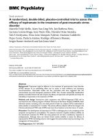
The results obtained from three gradient profiles are shown in
Fig. 1. The well-resolved chromatogram in Fig. 1a takes 26.5 min,

on the contrary, although the chromatogram in Fig. 1b takes less
time, it shows large overlapping between contiguous peaks. Fig. 1c
shows the chosen experiment as an adequate gradient profile to
separate and quantify the four primary aromatic amines.
Responses Y1 , Y2 and Y3 refers to the resolution (Rs) between
contiguous peaks at the emission wavelength of 350 nm, computed as in Eq. (1) with the peak identification in Fig. 1, Y1 = Rs12 ,
Y2 = Rs23 , Y3 = Rs34 . Y4 is the time which the chromatogram takes
(tf ), computed by the final time of the last eluted peak.
As the purpose of this work is to model through PLS the relationship between the elution conditions and the CQA of the chromatogram (which are the three resolutions and the final time), it
is necessary to maintain their values, even if they become negative
due to the crossing of some of the peaks under certain chromatographic conditions. If these resolutions are summarized in a single
index such as the usual "critical resolution", the perspective that
experimental data provides about the true relation between CMP
and CQA is altered. That is the reason why the peak assignation
is maintained: (1) ANL, (2) TDA, (3) MDA and (4) ABP even when
peak crossing between ANL and TDA occurs.
For the analysis of the extracts of napkins, to obtain data matrices for each analysed sample, software has been programmed
to record the whole emission spectra between 290 and 430 nm
(each 1 nm) for each elution time of the entire analysis. Therefore,
if there is any interferent in the samples, a multi-way technique
will be used, in this case PARAFAC, for the unequivocal identification of the PAAs.

2. Material and methods
2.1. Chemicals and reagents
Aniline (ANL ≥ 99.5%, CAS no. 62-53-3), 2,4-diaminotoluene
(TDA 98%, CAS no. 95-80-7), 4,4 -methylenedianiline (MDA ≥ 97%,
CAS no. 101-77-9), and 2-aminobiphenyl (ABP 97%, CAS no. 9041-5) were acquired in Sigma-Aldrich (Steinheim, Germany). Acetonitrile (CAS no. 75-05-8) and methanol (CAS no. 67-56-1), both
LiChrosolv® isocratic grade for liquid chromatography, were supplied by Merck (Darmstadt, Germany). Deionized water was obtained by using the Milli-Q gradient A10 water purification system
from Millipore (Bedford, MA, USA).
2.2. Instrumental

For the preparation of the extracts of PAAs, a water bath
equipped with a Digiterm 200 immersion thermostat (JP Selecta
S.A., Barcelona, Spain) was used. A rotary evaporator (ILMVAC, Ilmenau, Germany) was also employed for the pre-concentration of
the extracts, with a pressure of 72 mbar and a temperature between 50 and 60 °C for the elimination of water. A centrifuge
(Sigma Laborzentrifugen, Osterode, Germany) was used to separate
the possible remaining paper fibres in the sample.
The determination of the four primary aromatic amines, ANL,
TDA, MDA, and ABP, was carried out by using an Agilent 1260
Infinity HPLC chromatograph (Santa Clara, CA, USA) equipped
with a quaternary pump (G1311C), a sampler (G1329B), a thermostatic column compartment (G1316A), and a fluorescence detector (G1321B). An InfinityLab Poroshell 120 SB-C18 column
(150 × 4.6 mm, 4 μm), purchased by Agilent Technologies, was
used for the separation. Deionized water, methanol, and acetonitrile were used as mobile phases.
The conditions for chromatographic analyses were programmed
in gradient elution mode. Mobile phase consists of different percentages of a water:methanol:acetonitrile (A:B:C, v/v) mixture, depending on the conditions in the different experiments conducted,
which are explained in the following Sections 3.1 and 3.3, keeping
the mobile phase flow rate fixed at 0.5 mL min−1 and the column
temperature at 40 °C.
In every analysis, the injection volume was 10 μL. The fluorescence detector was programmed to measure the fluorescence
intensity at a fixed excitation wavelength of 225 nm. Four emission wavelengths were selected to better identification of the four
PAAs in chromatograms, being 310 and 342 nm the ones for ANL,
350 nm for TDA and MDA, and 385 nm for ABP. However, only the

2.3. Standard solutions
Individual standard stock solutions of 500 mg L−1 were prepared by dissolving each standard in methanol and they were
stored and protected from light at 4 °C. A mixture with different concentration levels of each PAA (4, 10, 6 and 1 mg L−1 for
ANL, TDA, MDA and ABP, respectively) was prepared from the standard stock solutions by dilution with methanol. This mixture solution was used for the exploratory experiments carried out and
explained in Section 3.1.
Once the more adequate conditions for the gradient profile
(Section 3.3) were selected, a univariate calibration model for each
primary aromatic amine was fitted using the integrated peak area

at 350 nm emission wavelength as response. For this task, ten calibration standards, four of them analysed in duplicate, were prepared. Firstly, individual stock solutions of 25 mg L−1 were prepared from the ones of 500 mg L−1 by dilution with methanol.
The ten calibration standards, which contained crossing concentration levels of each PAA, were prepared from the individual stock
solutions of 25 mg L−1 by dilution with methanol. These concentration levels were 0, 0.05, 0.1, 0.25, 0.5, 0.75, 1, 2, 3 and 4 mg L−1
for ANL; 0, 0.5, 0.75, 1, 1.5, 2, 4, 6, 8 and 10 mg L−1 for TDA; 0, 0.1,
0.25, 0.5, 0.75, 1, 1.5, 2, 4 and 6 mg L−1 for MDA; and 0, 0.1, 0.25,
3


M.M. Arce, D. Castro, L.A. Sarabia et al.

Journal of Chromatography A 1676 (2022) 463252

Fig. 1. Chromatograms obtained with different gradient profiles: (a) the one codified as 13 in column 1 in Table 1; (b) the one codified as 03 in column 1 in Table 1; (c) the
one codified as 36 in Table 3. Peak identification: (1) ANL, (2) TDA, (3) MDA and (4) ABP.

4


M.M. Arce, D. Castro, L.A. Sarabia et al.

Journal of Chromatography A 1676 (2022) 463252

0.5, 0.75, 1, 1.25, 1.5, 1.75 and 2 mg L−1 for ABP. These solutions
were stored and protected from light at 4 °C.

ues of the chromatographic gradient profiles applied in each of the
three cases are shown.
For the gradient defined by L and α , different gradient elution
profiles in time can be programmed. To obtain one of them, a maximum time ts for each segment and a total maximum time tt are
defined, and the g segments of the gradient (t1 , t2 , …, tg ), are generated, being ti (i = 1, …, g) an integer between zero and ts , chosen

g
randomly with uniform distribution and the restriction tt = i=1 ti ,
ti is the time that the composition of the mobile phase remains in
each segment of the gradient.
For instance, in order to obtain the chromatograms of Fig. 1, it
has been used g = 11, ts = 8 and tt = 35 min. The mixture diagrams show the values of L and α that define the trajectory from
the initial to the final composition, and the sequence of the 11 corresponding ternary mixtures, indicated using circles, for each case.
In Fig. 1a the second and the sixth mixtures are missing, because t2 = t6 = 0, as shown in row 13 in Table 1. The profile of the
percentage of methanol and acetonitrile in each segment is also
drawn, note that the four analytes have eluted in 26.5 min, so the
experimental profile only reaches the t9 .
This situation is more pronounced in the chromatogram of
Fig. 1b, whose experimental profile only needs until t3 (see row
3 in Table 1), because at 7 min all the analytes have eluted. Finally, Fig. 1c shows the profile of a binary water:methanol gradient
(experiment coded as 36 in Table 3), that starts with 30% organic
phase and ends at 100%. Once again, the experimental profile only
uses 8 of the 11 gradient profile times as all four analytes elute in
15.6 min.

2.4. Procedure to obtain the extract from napkins
For the quantification of PAAs in napkins (Section 3.4), more diluted calibration standards were needed. For this task, new calibration standards, two of them analysed in duplicate, were prepared.
Firstly, individual stock solutions of 1 mg L−1 for ANL, MDA and
ABP were prepared from the ones of 25 mg L−1 by dilution with
methanol. The calibration standards were prepared from the individual stock solutions of 1 mg L−1 for ANL, MDA and ABP and of
25 mg L−1 for TDA by dilution with methanol. These concentration
levels were 2.5, 5, 10, 15, 20, 35 and 50 μg L−1 for ANL; 50, 100,
20 0, 30 0, 40 0, 50 0 and 60 0 μg L−1 for TDA; 10, 20, 30, 45, 60, 80,
100 and 250 μg L−1 for MDA; 10, 20, 30, 45, 60, 80 and 100 μg L−1
for ABP. Moreover, for some extracts of napkins, it was necessary
to prepare more concentrated calibrations standards: 0.1, 0.5 and

1 mg L−1 for ANL; 0.75, 1.5 and 4 mg L−1 for TDA. These solutions
were also stored and protected from light at 4 °C.
The preparation of the extracts of the three types of napkins
was carried out following the UNE-EN 647 standard in force [32],
which indicates how to extract PAAs from paper and cardboard
materials intended to come into contact with food. 10 g of each
napkin, previously cut into pieces between 1 and 2 cm2 , were
weighed and placed in an Erlenmeyer flask, where 200 mL of water were added. The extraction process was carried out in a water
bath at 80 ± 2 °C.
After 2 h, the solution was decanted, and the sample residues
retained in the flask were washed several times. Subsequently, the
solution was filtered with a filter plate of porosity 4 (ranged 5 to
15 μm). This filtrate was transferred to a 250 mL volumetric flask,
filling up to the mark with water. Water was removed from the
samples with a rotary evaporator to obtain the corresponding PAA
extracts. These extracts were reconstituted in methanol, filling up
to 10 mL in a volumetric flask and then centrifuged for 3 min at
60 0 0 rpm and at 10 °C to separate the possible remaining paper
fibres in the sample.

2.6. Software
The set-up of a ternary gradient profile has been programmed
as a GUI in MATLAB [33]. The source code is freely available via
GitHub [34] and is described in the Supplementary Material. OpenLab CDS ChemStation software was used for acquiring data. The
PLS Toolbox [35] for use with MATLAB [33] was employed for fitting PLS models and to carry out PARAFAC2 decompositions. The
regression models were fitted and validated applying STATGRAPHICS Centurion 18 [36]. Decision limit (CCα ) and detection capability
(CCβ ) were calculated using the DETARCHI program [37].

2.5. Gradient modelling
3. Results and discussion

The feasibility of using a gradient elution profile to approximate
any possible gradient elution program, linear or not, has already
been shown in Ref. [19]. To do that, once the range between the
lowest and highest proportion of modifier in the mobile phase has
been decided, the chromatogram is described by g proportions of
the modifier obtained by dividing the total range into g equal segments. By varying the duration of each of these g segments of the
chromatogram, a suitable model is obtained to describe the gradient elution using ternary solvent mixtures.
By using the codification described in Ref. [19], a procedure has
been developed to set up a gradient profile that makes possible
to plan the exploration of the ternary water:methanol:acetonitrile
mobile phase. Each chromatogram will be encoded by two parameters, L and α .
L defines the binary mixture whose composition is the beginning of the mobile phase gradient profile. L takes values between
0 and 200, where L = 0 is 100% methanol, L = 100 is 100% water
and L = 200 is 100% acetonitrile.
α is the angle formed by the line defining the gradient profile
and the horizontal depicted from L. α can take values between 0
and 120 °, coinciding 0 ° with the horizontal and 120 ° with the
side of the triangle. Note that when L ∈ (0, 100), α is oriented
clockwise, while when L ∈ (10 0, 20 0) it is oriented counterclockwise. In Fig. 1, in addition to the chromatograms, the L and α val-

3.1. Exploration of experimental domain
When designing the experimentation, its practical viability in
terms of analysis time must be contemplated. It was considered
acceptable to use three sessions of 8 h. This, resulted in limiting the chromatograms for the construction of the PLS model to
30 and the validation of the proposed solutions to 7. In practice,
including some failed experiments and stabilisation time, all 37
chromatograms were done in less than 26 h. To evaluate this experimental effort, it is necessary to take into account the search
space has 33 dimensions (composition of methanol an acetonitrile
and time of each of the 11 segments considered), so, it cannot be
considered excessive to explore it with 30 experiments. The search

space could be reduced with previous knowledge, for example, if
the percentage of water cannot be greater than 60%, the number
of initial trials will be reduced to 20.
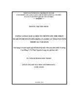
The initial exploration has been carried out with the 20 gradients shown in Fig. 2a, where the black points indicate the values
of L (10, 30, 60, 90, 110, 140, 170 and 190) and the colours, the
different values of α (0 ° in red, 30 ° in pink, 60 ° in blue, 80 °
in yellow, 90 ° in orange and 120 ° in green). The design that has
been used, is a modification of the theoretical D-optimal design
for 20 experiments with 8 and 6 levels of L and α , respectively.
5


M.M. Arce, D. Castro, L.A. Sarabia et al.

Journal of Chromatography A 1676 (2022) 463252

Table 1
L, α and ti parameters that define the gradient profile used for each one of the 30 exploration experiments carried out in the laboratory, and the four
responses calculated from the chromatogram obtained in each case.
Code Fig. 2(a)

Code Table S1
∗

#

L

α

t1

t2

t3

t4

t5

t6

t7

t8

t9

t10

t11

Y1

Y2

Y3

Y4

10

0

2

3

5

3

3

3

1

3

5

5

2

0.00

0.00

2.05

3.996

30
30
30
30

0
0
30
60

4
5
1
1

2
0
3
3

4
4
6
1

4

3
6
0

1
5
5
5

4
2
2
3

5
4
4
5

3
4
0
4

4
1
1
3

3

2
1
5

1
5
6
5

0.93
0.00
0.00
0.00

0.96
1.55
1.83
1.63

8.18
7.65
8.55
8.18

6.822
6.840
6.642
6.674

01

20

02
03
04
05

13
16
14
15

06
07
08
09
10
11

05
09
06
07
23
08

60
60
60

60
60
60

0
0
30
60
60
120

4
4
1
1
1
1

2
3
1
0
0
1

2
1
6
0
0

5

2
5
4
0
0
0

5
2
3
3
3
3

5
0
4
4
4
3

1
6
3
3
3
6

3
2
4
6
6
3

3
3
3
5
5
3

3
6
4
6
6
5

7
5
2
7
7
5

-1.15
-1.43

-1.07
-0.86
-1.30
-1.24

14.16
13.65
9.92
5.61
5.88
9.19

26.67
25.16
20.43
12.72
14.20
18.90

36.421
35.665
19.303
10.436
10.198
15.635

12
13
14
15

16
17

01
12
22
27
02
28

90
90
90
90
90
90

80
80
80
80
120
120

5
5
5
0
6
0

0
0
0
8
2
0

4
4
4
8
0
1

3
3
3
4
1
0

7
7
7
8
6
1

0

0
0
1
4
4

3
3
3
4
1
6

3
3
3
0
3
4

3
3
3
0
5
6

5
5
5

1
1
8

2
2
2
3
6
5

-4.17
-3.81
-4.33
-2.88
-3.88
-1.77

22.11
20.33
23.09
23.69
18.78
9.85

18.75
16.94
19.45
26.25
22.61

16.52

26.338
26.505
26.529
35.341
26.021
15.127

18
19
20
21

03
29
04
30

110
110
110
110

80
80
120
120

7

0
4
0

2
4
4
4

5
0
6
4

1
7
1
4

2
2
4
4

0
4
1
3

4

0
1
5

4
6
4
5

3
2
3
0

3
4
3
5

4
6
4
1

-1.82
-1.27
-1.54
-1.04

17.26

19.40
15.36
15.07

16.51
19.99
16.40
19.51

26.032
22.828
25.895
23.429

22
23
24

24
10
11

∗

140
140
140

0
60

90

4
5
2

3
3
5

1
5
2

5
5
2

2
3
2

0
0
5

6
2
4

2
3
2

3
2
1

6
1
5

3
6
5

0.00
0.92
0.93

7.65
4.83
4.21

17.02
13.78
15.75

26.253
16.567

14.724

25
26
27
28

25
17
18
19

#
#
#
#

170
170
170
170

0
30
60
120

4
4
4

5

2
4
4
5

4
3
6
1

4
1
4
5

1
3
0
3

4
0
1
0

5
3
5

1

3
3
2
3

4
4
5
5

3
5
1
5

1
5
3
2

1.26
1.06
1.43
1.62

0.00
0.00
0.00

0.00

5.05
5.01
4.80
4.76

5.454
5.486
5.494
5.512

29
30

21
26

∗

190
190

0
0

5
5

2

2

4
4

1
1

2
2

5
5

4
4

5
5

3
3

0
0

4
4

0.00

0.00

0.00
0.00

1.37
1.32

3.881
3.863

∗
∗
∗

∗

#
#

(∗ ) Experiments excluded for modelling Y1 .
(#) Experiments excluded for modelling Y2 .

Fig. 2. Directions defined by L and α parameters for different gradient profiles. (a) The 20 ones used for the 30 exploratory experiments carried out in the laboratory and
(b) the 14 ones used for the 21 out of 45 proposed conditions for prediction.

6


M.M. Arce, D. Castro, L.A. Sarabia et al.

Journal of Chromatography A 1676 (2022) 463252
Table 2
PLS models fitted for each experimental response with data from Table 1. L.V., number of latent variables, R2 , variance explained of Y block in fitting, R2 c.v., variance
explained of Y block in cross-validation. P-value is the significance for the crossvalidated permutation tests.

As shown in Fig. 2a, the number of gradients has been reduced
to two when L = 90 or L = 110, because a long final time is expected under these conditions. Also, only a single gradient (α = 0
°) is considered when methanol and acetonitrile are, respectively,
at 90% (L = 10 and L = 190) because the variation in the range of
ternary mixtures is very small. The design used is a compromise
between the statistical properties of the D-optimal design and the
analytical meaning of L and α .
As it can be seen, for the same value of L, the chromatograms
for different values of α have been recorded. Four replicates of
some pairs of values of L and α have been performed (experiments
coded as 10, 13, 14 and 30). Also, the analysis has been completed
by generating different series of ti in six pairs of L and α values
(experiments coded as 03, 07, 15, 17, 19 and 21 in Fig. 2a and in
Table 1, column 1). Therefore, a total of 30 chromatograms were
recorded in the laboratory.

Response L.V. R2

R2 c.v.

Var. explained
X block (%)

P-value

W∗

S∗ ∗

R∗ ∗ ∗

Y1
Y2
Y3
Y4

0.8138
0.8499
0.7928
0.8034

77.40
73.58
73.40
72.60

0.001
0.002
0.001
<0.0005

0.013
0.014
0.005
0.002

0.006
0.005
0.006
0.005

(Rs12 )
(Rs23 )
(Rs34 )
(tf )

4
4
4
4

0.9418
0.9640
0.9207
0.9341

(∗ ) Pairwise Wilcoxon signed rank test.
(∗ ∗ ) Pairwise signed rank test.
(∗ ∗ ∗ ) Randomisation t-test.

ing three permutation tests (50 iterations) using the residuals in
cross-validation, because they are more sensitive to detect overfitting. The p-values reported in Table 2 vary between 0.0 0 05 and
0.014. That is, the model fitted for each Yi , i = 1, …, 4 is distinguishable from one created randomly shuffling the response at a
confidence level between 0.9995 and 0.986 which is a level much
higher than usual 0.95.

Once the PLS models have been built, the multi-segmented gradient profile is analysed for each L and α in relation to the resolutions and final time obtained, their confidence intervals and
the desired CQA values. Based on this, 24 new gradients are proposed which come from previous directions of the training set
(Fig. 2a) but with a time profile of the gradient (t1 , t2 , …, tg ) chosen based on the experimental results already obtained. Some others are added in order to explore promising regions of L and α
values. In this case there are 21 corresponding to 14 new directions shown in different colours in Fig. 2b, where the values of L
studied (20, 30, 40, 70, 100, 150, 160 and 180) have been marked
again with black points and the α values with different colours (0
° in red, 15 ° in pink, 60 ° in blue, 90 ° in orange and 120 ° in
green). For five pairs of L and α values, other different series for ti
have been generated. Remember that the space to be explored has
33 dimensions, so testing different profiles for the gradient implies
handling 33 parameters. These gradient profiles and the calculated
values Yˆi , i = 1,..., 4 obtained with the PLS models can be consulted
in Table S1 in Supplementary Material.
It is known that PLS regression, like all least squares methods, makes predictions of average values, not individual ones. This,
along with the large dimensionality of the search space and the reduced number of chromatograms, causes large confidence intervals
for the estimated values of the resolutions and final time which
has already been confirmed in the case of isocratic elution [15].
This fact can be seen in Fig. 3 which shows the confidence intervals calculated at 95% confidence level. In this specific case, it is
imposed, to the predictions obtained from the 75 chromatograms,
that the resolutions must be greater or equal to 1.5 in absolute
value and that the final time less than 20 min. Taking this into
account, seven proposals have been found that fulfil both requirements (marked with the corresponding code in Table 3). The necessity to consider not the mean value but the interval is shown,
for example, in chromatograms 75, 44, 46 whose estimates together with their confidence intervals do not guarantee that Rs23
is greater than 1.5, as occurs experimentally (Table 3).

3.2. Fitting and analysis of a PLS prediction model
In each of the 30 chromatograms, defined by the previous gradient profiles, four responses have been obtained that define the
quality of the chromatogram: the three resolutions between contiguous peaks (Y1 , Y2 , Y3 ) and the final time (Y4 ) (see details
in Section 2.2). The experimental values obtained are shown in
Table 1. As it can be seen, there is a tendency depending on the

value that L takes. For Y4 (tf ) the lowest values are obtained with
the extreme values of L (close to 0 and 200), and as L approaches
to 100, these times increase. But the effect of α is also appreciated,
for example, for L = 60 Y4 varies from 36 to 10 min.
The time profile effect on the gradient is also observed, for example for L = 90 and α = 120 ° (binary water:methanol phase) the
resolution Rs12 (Y1 in Table 1) is halved when changing the time
profile from chromatogram 16 to 17. The other two resolutions Y2 ,
Y3 and the final time Y4 are also reduced. In addition, the chromatograms with the lowest final time (L = 10, 30, 170 and 190)
have poor Rs12 and/or Rs23 resolutions. For values close to L = 100,
resolutions are better, ensuring the separation of the analytes, but
the time tf is increased.
Based on the experimental results, it is clear that the optimal ternary gradient elution profile is different depending on the
characteristic of the chromatogram considered: resolutions or final
time. To find a solution of compromise, it is proposed to fit a prediction model using the 33 predictor variables that correspond to
the 11 ti values and the different percentages of methanol and acetonitrile that define the conditions of each one of the 30 recorded
chromatograms. Since these 33 predictors are correlated, it is appropriate to consider a partial least squares (PLS) model. Therefore,
a model is fitted for each of the resolutions and for the final time.
Some considerations have been taken into account, Y1 has a value
of zero in seven chromatograms, which indicates that, with those
experimental conditions, the Rs12 resolution cannot be modelled.
That also happens with other seven chromatograms for Rs23 . For
Y1 and Y2 the model has been fitted with the 23 non-null values,
excluding the chromatograms marked in Table 1 with (∗ ) or (#),
respectively. For answers Y3 and Y4 it has been possible to use the
30 chromatograms.
The characteristics of the fitted models are shown in Table 2.
The number of latent variables was chosen by leave one out crossvalidation procedure, being necessary 4 latent variables for each
model. The global percentage of variance explained in training
varies between 92 and 96% and in cross-validation, varies from 79
to 85%. As a reference, in the PLS models of [25] the R2 values

obtained are ranged from 0.942 to 0.994, quite similar to the values obtained in the present work between 0.921 and 0.964. These
models only need between 72 and 77% of the variance of the 33
predictors. The absence of overfitting has been evaluated by do-

3.3. Experimental verification of the predictions
Once these seven conditions were selected, the corresponding
chromatograms were recorded in laboratory. The results obtained
for each of the four responses are shown in Table 3. As it can
be seen, three conditions of the proposals do not fulfil the prediction of Rs23 (Y2 ), chromatograms with code 75, 44 and 46. Of
7


M.M. Arce, D. Castro, L.A. Sarabia et al.

Journal of Chromatography A 1676 (2022) 463252

Fig. 3. For the 30 exploratory experiments (in black) and the 45 proposed conditions (in red), predicted values and its confidence interval at 95% confidence level calculated
from the PLS models for (a) Rs12 , (b) Rs23 , (c) Rs34 and (d) tf .
Table 3
L, α and ti parameters that define the gradient profile used for each of the seven validation experiments carried out in the laboratory, and the
four responses calculated from the chromatogram obtained in each case.
Code Table S1 Fig. 3

L

α

t1

t2

t3

t4

t5

t6

t7

t8

t9

t10

t11

Y1

Y2

Y3

Y4

75
38
55

36
28
44
46

20
60
70
70
90
170
170

0
60
120
120
120
0
120

4
1
0
1
0
6
8

2

0
1
0
0
3
7

4
2
0
1
1
4
1

1
4
1
4
0
4
5

2
3
4
3
1
1
3

8
0
3
0
4
4
0

4
0
0
4
6
5
1

5
6
4
5
4
3
3

1
6
6
5
6

1
5

0
6
8
6
8
3
0

4
7
8
6
5
1
2

0.69
-1.47
-1.59
-2.10
-1.92
1.48
1.26

0.00
9.17
9.12

13.46
11.41
0.00
0.00

5.09
19.60
21.58
19.73
18.43
5.26
5.53

4.867
13.792
13.921
15.624
15.041
5.504
5.494

the remaining four proposals, as there is not much difference between the final time obtained, the chromatographic conditions of
case 36, that have better resolution Rs12 (Y1 ), are chosen. To decide
if the PLS model provides resolutions and final time values similar to the experimental ones, the four regressions Yi (estimated
value with PLS) versus Yi (experimental value), i = 1, 2, 3, 4 have
been built. The null hypothesis that states the estimated and experimental values are the same, cannot be rejected (at the 0.05
level of significance) as shown in Table 4. Despite having explored

ternary mixtures, the optimisation leads to a gradient profile of
water:methanol binary mixtures.

Under these conditions, a univariate calibration model is built
(using the peak area as response) with ten concentration levels
(explained in Section 2.3). Table 5 shows the parameters of the
calibration and accuracy lines for each PAAs. All of them are significant models, without lack of fit at 95% confidence and they are
also unbiased because intercepts are equal to zero and slopes equal
to one.

8


M.M. Arce, D. Castro, L.A. Sarabia et al.

Journal of Chromatography A 1676 (2022) 463252

Table 4
Parameters of the regression models (predicted data versus experimental results) fitted for the four responses considered.

Number of data
Intercept
Slope
Correlation coefficient
P-value (H0 : Intercept equal to zero and slope equal to one)

Y1 (Rs12 )

Y2 (Rs23 )

Y3 (Rs34 )

Y4 (tf )

30
-0.0010
0.9924
0.9661
0.9861

30
-1.0057
1.0635
0.9648
0.3627

37
1.4378
0.8723
0.9374
0.0612

37
1.8218
0.9048
0.9581
0.1007

Table 5
Performance criteria of the analytical method. Parameters of calibration (fitted with peak areas as response) and accuracy lines (syx is the standard
deviation of regression).

Calibration

line

Accuracy line

Linear range (mg L−1 )
Intercept
Slope
Correlation coefficient
syx
P-value (H0 : Regression is not significant)
P-value (H0 : There is not lack of fit)
P-value (H0 : Intercept equal to zero and slope equal to one)

TDA n = 14

MDA n = 14

ABP n = 14

0–4
2.4091
104.05
0.9999
2.1806
<10−4
0.2489
1.0000

0–10
-4.8377

7.9798
0.9928
3.3250
<10−4
0.5086
1.0000

0–6
0.8839
18.674
0.9995
1.0711
<10−4
0.1122
1.0000

0–2
-0.0389
19.660
0.9999
0.2253
<10−4
0.4457
1.0000

Chromatographic data are trilinear if the experimental data array is compatible with the structure in Eq. (2). The core consistency diagnostic (CORCONDIA) [45] measures the trilinearity degree of the experimental three-way array when F ≥ 2. If the threeway array is trilinear, then the maximum CORCONDIA value of
100% is achieved. Additionally, the trilinearity is verified by using partitions in the data set (split-half analysis), the variance explained and the chemical coherence of the three profiles [42,45].
The PARAFAC solution is unique when the three-way array is
trilinear and the appropriate number of factors has been chosen to fit the PARAFAC model [42]. The uniqueness property, also
known as "second order property" makes it possible to identify

compounds unequivocally by their chromatographic and spectral
profiles as laid down in some official regulations and guidelines
[38,46,47], even in the presence of a coeluent that appears with
the analyte of interest.
However, PARAFAC2 is used to correct deviations from trilinearity when small shifts in the retention time of the analytes from
sample to sample appear in the chromatogram [48,49]. In this case,
PARAFAC2 applies the same profiles (bf , f = 1,…,F) along the spectral mode and enables the chromatographic mode to vary from one
matrix to another.
Then, Eq. (2) should be modified as in Eq. (3) to describe a
PARAFAC2 model:

3.4. Application to samples
Once the validation of the method has been verified, it is applied to the determination of the four primary aromatic amines in
extracts obtained from paper napkins.
The samples obtained from the extracts of paper napkins have a
complex matrix. For this reason, it is necessary to apply a chemometric technique with the second order advantage, which means
it provides the unequivocal identification of the analytes, even in
the presence of non-modelled interferents. There are several papers that show the advantage of applying the PARAFAC/PARAFAC2
decomposition technique to data obtained from samples with a
complex matrix [38–41]. This technique is applied to three-way
data tensors (I × J × K) that can come from different instrumental
methods (HPLC-DAD, HPLC-FLD, GC-MS, EEM, etc) [42].
3.4.1. PARAFAC/PARAFAC2 models
In general, a three-way data array X of dimension I × J × K is
made up of real numbers, xijk , i = 1,…, I; j = 1,…, J; k = 1,…, K. A
PARAFAC model of rank F for the data array X = (xijk ) is written
[43,44] as Eq. (2):
F

xi jk =

ANL n = 14

ai f b j f ck f + ei jk , i = 1, 2, . . . , I; j = 1, 2, . . . , J; k = 1, 2, . . . , K
f =1

F

akif bjf ckf + eijk , i = 1, 2, . . . , I; j = 1, 2, . . . , J;

X = xijk =

(2)

f =1

where ei jk are residuals of the fitted model. PARAFAC is a trilinear
model, as can be seen in Eq. (2), since it is linear in each of the
three profiles (or ways). HPLC-FLD data can be arranged for each
chromatographic peak in a three-way array X and analysed with
the PARAFAC decomposition technique. In this case, the dimension
of the data tensor X is I × J × K, where for each of the K samples analysed, the intensity measured at J wavelengths is recorded
at I elution times around the retention time of every compound.
According to Eq. (2) PARAFAC decomposes a HPLC-FLD data tensor X into F factors and each factor consists of three loading vectors af , bf and cf , (f = 1, 2,…F) with dimensions I (elution times), J
(wavelengths) and K (number of samples) respectively. In practice,
each profile (way or mode) of the array is identified by its meaning, for example, chromatographic, spectral or sample profiles for
HPLC-FLD data. The order of the profiles is not predetermined, and
the researcher decides it.

k = 1, 2, . . . , K

(3)

where the superscript k is added to account for the dependence of
the chromatographic profile on the k-th sample.
In the construction of the PARAFAC/PARAFAC2 model, constraints on the profiles can be imposed, for example, nonnegativity.

3.4.2. PARAFAC2 models for PAAs
As already mentioned before, in this work the three profiles of
the arranged tensors of dimension (I × J × K) correspond to chromatographic (I), spectral (J) and sample (K) profiles, respectively.
It has been observed that for all of them the application of the
PARAFAC2 decomposition has been necessary because of the retention time shifts.
9


M.M. Arce, D. Castro, L.A. Sarabia et al.

Journal of Chromatography A 1676 (2022) 463252

Table 6
Characteristics of the PARAFAC2 decomposition models obtained for the determination of the four PAAs in napkins.

Analyte
ANL
TDA

MDA
ABP

Time window

(min)

I×J×K

7.00–7.31
7.00–7.31
6.55–6.85
6.55–6.85
6.55–6.85
10.75–11.00
15.25–15.55

59
59
57
57
57
47
56

×
×
×
×
×
×
×

141
141

141
141
141
141
141

×
×
×
×
×
×
×

13
10
13
11
14
18
17

Number of
factors

Variance of
CORCONDIA (%) X (%)

Split-half
analysis (%)

Correlation
coefficient
(n = 141)

Concentration
range (μg L−1 )

Napkin

2
2
2
2
3
3
3

100
100
100
100
98
99
98

99.8
95.5
93.6
98.2

97.5
95.7
96.8

0.9988
0.9962
0.9864
0.9826
0.9637
0.9978
0.9993

0–50
0–1000
0–600
0–4000
0–750
0–250
0–100

Nap1
Nap2, Nap3
Nap1
Nap2
Nap3
Nap1, Nap2, Nap3
Nap1, Nap2, Nap3

99.82
99.64

99.59
99.89
99.90
99.90
99.90

Columns 1 and 2 in Table 6 detail the time window selected
for each analyte and each arranged tensor, while column 3 shows
its dimensions. The size of the spectral profile (J) is always 141,
which corresponds to the emission wavelengths between 290 and
430 nm. However, the size of the chromatographic and sample profiles, differ from one tensor to another depending on the time window of the chromatogram (I) and the number of samples included
in each considered tensor (K), which depends on the napkin samples considered (column 10 in Table 6) and the calibration range of
the standard samples (column 9 in Table 6).
Once the tensors are arranged, the PARAFAC2 decomposition is
carried out. For all models, a non-negativity constraint was applied in the three profiles, with the exception of the model for
ABP (last row in Table 6), where it was imposed the non-negativity
constraint just in the sample profile. Each one of the seven models were fitted with the number of factors shown in column 4 in
Table 6. This number of factors was chosen using the CORCONDIA index, the percentage of variance explained, and the similarity
found when performing the split-half analysis (columns 5, 6 and
7 respectively). The values obtained for the CORCONDIA index are
close to 100% in the seven cases, explaining, at least, the 99.59% of
variance and with a similarity that varies between 93.6 and 99.8%,
which indicates that the PARAFAC2 decomposition is adequate.
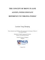
Fig. 4 shows, as an example, the PARAFAC2 model for ABP.
Fig. 4a shows the chromatographic profile, Fig. 4b the spectral one
and Fig. 4c the sample one, being the blue factor the analyte and
the orange and yellow ones the interferents.
As indicated in the model of Eq. (3), PARAFAC2 estimates a
chromatographic profile af k for each k sample and each f factor. In this case there are three factors (F = 3) identified by the
colour code, and for each of them, 17 chromatographic profiles

(shown in Fig. 4a). It is evident that only the blue profile shows
the typical appearance of a chromatogram, while the estimated
chromatograms for the interferents are poorly distinguishable from
noise. In other words, in the chromatographic peak of the ABP, no
deformation caused by the interferents would be perceptible. Continuing with Eq. (3), the spectral profile estimates the three fluorescence spectra, bf , common to all samples shown with the same
colour code in Fig. 4b. These are well-shaped spectra that are recognizable, particularly the ABP one. Finally, Fig. 4c shows the corresponding values of the three sample loadings, cf , f = 1, 2, 3. It
is observed that in the calibration samples, the loading increases
with the concentration, in fact this allows the calibration by representing the associated ABP loadings (in blue) versus the true ABP
concentration of the calibration standards.
The unequivocal identification of each amine, is done by comparing the chromatographic and spectral profiles, obtained with
the PARAFAC2 decomposition, with those of a reference sample
analysed in the laboratory.
On the one hand, in the case of the chromatographic profile, the usual criteria of many European regulations on veterinary
residues and/or pesticides [46,47] has been followed, therefore, the
retention time obtained with PARAFAC2 decomposition, must cor-

respond to the retention time of a reference sample, admitting a
tolerance of ± 0.1 min. PARAFAC2 technique has been used, so,
a chromatographic profile is obtained for each sample of the tensor. Considering the retention time of the reference samples (ANL
7.254 min, TDA 6.762 min, MDA 10.964 min and ABP 15.351 min),
all the chromatographic profiles fulfil the aforementioned premise.
Additionally, in the case of the spectral profile, the unequivocal
identification has been carried out through the correlation coefficient. The values obtained for each of the tensors arranged are
shown in column 8 in Table 6, being all of them close to 1, what
guarantees the identity of the amine.
3.4.3. Performance criteria
Once the factor that corresponds to each analyte has been identified, its sample loadings are used for calibration as the instrumental signal, in order to carry out the regression of loadings versus true concentration. Although the corresponding calibration and
accuracy lines (concentration obtained with PARAFAC2 versus true
concentration) have been fitted and validated for each tensor used,
Table 7 only shows those used to calculate the decision limit (CCα )

and the detection capability (CCβ ) for each analyte, which corresponds to rows 1, 3, 6 and 7 in Table 6. The calibration models
are significant and do not show lack of fit at a confidence level of
95%, except for the MDA (see rows 6 and 7 in Table 7). However,
the corresponding accuracy line indicates that the MDA concentration values predicted versus the true concentration, are significantly the same (row 11 in Table 7). The method is validated by
means of the accuracy lines, being the p-values of the joint hypothesis test (H0 : Intercept equal to zero and slope equal to one)
greater than 0.05, and the precision is the residual standard deviation (syx ) (rows 11 and 5 of the same table). Therefore, the method
is unbiased. The last two rows of Table 7 show the values of CCα
and CCβ for each PAA, being the probability of false positive and
false negative equal to 0.05. It can be seen that TDA is the least
sensitive amine and that this method, although it only allows the
quantification of amounts greater than 189.4 μg L−1 of TDA, is capable of quantifying concentrations close to 2 μg L−1 of ANL.
3.4.4. Primary aromatic amines in napkins
For each tensor used (see Table 6), the corresponding calibration and accuracy lines have been fitted and validated in order to
predict the amount of each PAA in the napkin samples. The range
of calibration standards is different for each of these regressions,
depending on the concentration of each amine present in each
napkin.
ANL has been found in the three napkins, in quite different
amounts, 33.5, 619.3 and 77.7 μg L−1 . In the case of TDA, it is not
detected in Nap1, while quantities of 1907.9 and 725.9 μg L−1 have
been found in the others. However, MDA and ABP have not been
detected in any napkin. In all the cases, the higher concentrations
correspond to the recycled fibre napkin.
The concentrations found exceed the migration limit established in the European regulations for FCM of paper and cardboard
10


M.M. Arce, D. Castro, L.A. Sarabia et al.

Journal of Chromatography A 1676 (2022) 463252

Fig. 4. Loadings of the PARAFAC2 model obtained for ABP: (a) chromatographic, (b) spectral and (c) sample profiles, being the blue factor the analyte and the orange and
yellow ones the interferents.
Table 7
Performance criteria of the analytical method. Parameters of calibration (fitted with sample loadings as response) and accuracy lines (syx is the
standard deviation of regression). Decision limit (for α = 0.05) and detection capability (for α = β = 0.05).

Calibration
line

Accuracy
line

CCα (μg L−1 )
CCβ (μg L−1 )

−1

Linear range (μg L )
Intercept
Slope
Correlation coefficient
syx
P-value (H0 : Regression is not significant)
P-value (H0 : There is not lack of fit)
Intercept
Slope
syx
P-value (H0 : Intercept equal to zero and slope equal to one)

of 0.01 mg kg−1 [3,4]. Moreover, for the Nap2 napkin, which is a
recycled fibre napkin, the established limit of 0.1 mg kg−1 [5] is
also exceeded.

ANL n = 11

TDA n = 10

MDA n = 10

ABP n = 11

0–50
0.4291
0.3806
0.9994
0.2289
<10−4
0.1792
6.09 10−7
1.0000
0.6014
1.0000
0.916
1.786

0–600
0.4630
0.0076
0.9682

0.4485
<10−4
0.7967
2.50 10−5
1.0000
58.958
1.0000
97.4
189.4

0–250
-0.1842
0.0484
0.9924
0.4617
<10−4
0.0006
-3.03 10−6
1.0008
9.5394
0.9997
14.81
28.80

0–100
3.3563
1.4470
0.9996
1.4155
<10−4

0.6551
2.12 10−6
1.0000
0.9783
1.0000
1.537
2.998

the link to the tool MEG (multi-segmented elution gradient) developed ad-hoc for this work, freely available via GitHub. This tool allows the set up and the graphically display of the binary or ternary
gradient profile desired by the researcher.
Initially, 30 different gradient profiles were explored, and from
the results obtained for each of the four responses studied, four individual PLS models were fitted and validated. These models were
used to predict these 30 and other 45 new profiles. With the predictions obtained, the gradient profile that provided the best resolutions in the shortest analysis time was selected.

4. Conclusions
In this work, the search for an adequate chromatographic gradient profile that allows the separation of four primary aromatic
amines in a short analysis time by means of liquid chromatography
with fluorescent detection has been proposed. The paper includes
11


M.M. Arce, D. Castro, L.A. Sarabia et al.

Journal of Chromatography A 1676 (2022) 463252

The method has been applied to determine the concentration
of four PAAs in extracts obtained from three types of paper napkins, one of them made of recycled fibres. Due to the complexity
of the matrix, the application of the PARAFAC2 decomposition was
necessary to separate the interferents that eluted with the PAAs of
interest. The proposed method allows the quantification of concentrations above 1.8, 189.4, 28.8 and 3.0 μg L−1 of ANL, TDA, MDA

and ABP, respectively (for false positive and false negative fixed
at 0.05). ANL has been detected in the three napkins analysed in
quantities between 33.5 and 619.3 μg L−1 , while TDA is present
in only two napkins in quantities between 725.9 and 1908 μg L−1 .
In every case, the amount of PAAs found, exceeded the migration
limits established in European regulations.

[7] L. Rubio, S. Sanllorente, L.A. Sarabia, M.C. Ortiz, Optimization of a headspace
solid-phase microextraction and gas chromatography/mass spectrometry procedure for the determination of aromatic amines in water and in polyamide
spoons, Chemom. Intell. Lab. 133 (2014) 121–135, doi:10.1016/j.chemolab.2014.
01.013.
[8] V. Devreux, S. Combet, E. Clabaux, E.D. Gueneau, From pigments to coloured
napkins: comparative analyses of primary aromatic amines in cold water extracts of printed tissues by LC-HRMS and LC-MS/MS, Food Addit. Contam. A
37 (11) (2020) 1985–2010, doi:10.1080/19440049.2020.1802068.
[9] M. Shahrestani, M.S. Tehrani, S. Shoeibi, P.A. Azar, S.W. Husain, Comparison
between different extraction methods for determination of primary aromatic
amines in food simulant, J. Anal. Methods Chem. 2018 (2018) 1651629, doi:10.
1155/2018/1651629.
[10] A. Arrizabalaga-Larrañaga, P. de Juan-de Juan, C. Bressan, M. VázquezEspinosa, A.V. González-de-Peredo, F.J. Santos, E. Moyano, Ultra-highperformance liquid chromatography-atmospheric pressure ionization-tandem
mass spectrometry method for the migration studies of primary aromatic
amines from food contact materials, Anal. Bioanal. Chem. 414 (2022) 3137–
3151, doi:10.10 07/s0 0216- 022- 03946- 3.
[11] M.A.F. Perez, M. Padula, D. Moitinho, C.B.G. Bottoli, Primary aromatic amines
in kitchenware: determination by liquid chromatography-tandem mass spectrometry, J. Chromatogr. A 1602 (2019) 217–227, doi:10.1016/j.chroma.2019.05.
019.
˝ C. Kirchkeszner, N. Petrovics, Z. Nyiri, Z. Bo[12] B.S. Szabó, P.P. Jakab, J. Hegedus,
dai, T. Rikker, Z. Eke, Determination of 24 primary aromatic amines in aqueous food simulants by combining solid phase extraction and salting-out assisted liquid–liquid extraction with liquid chromatography tandem mass spectrometry, Microchem. J. 164 (2021) 105927, doi:10.1016/j.microc.2021.105927.
[13] S. Merkel, O. Kappenstein, S. Sander, J. Weyer, S. Richter, K. Pfaff, A. Luch,
Transfer of primary aromatic amines from coloured paper napkins into four
different food matrices and into cold water extracts, Food Addit. Contam. A

35 (6) (2018) 1223–1229, doi:10.1080/19440049.2018.1463567.
[14] M.M. Arce, S. Ruiz, S. Sanllorente, M.C. Ortiz, L.A. Sarabia, M.S. Sánchez, A
new approach based on inversion of a partial least squares model searching
for a preset analytical target profile. Application to the determination of five
bisphenols by liquid chromatography with diode array detector, Anal. Chim.
Acta 1149 (2021) 338217, doi:10.1016/j.aca.2021.338217.
[15] M.M. Arce, S. Sanllorente, S. Ruiz, M.S. Sánchez, L.A. Sarabia, M.C. Ortiz,
Method operable design region obtained with a partial least squares model
inversion in the determination of ten polycyclic aromatic hydrocarbons by liquid chromatography with fluorescence detection, J. Chromatogr. A 1657 (2021)
462577, doi:10.1016/j.chroma.2021.462577.
[16] N. Rácz, I. Molnár, A. Zöldhegyi, H.J. Rieger, R. Kormány, Simultaneous optimization of mobile phase composition and pH using retention modeling
and experimental design, J. Pharm. Biomed. 160 (2018) 336–343, doi:10.1016/
j.jpba.2018.07.054.
[17] H.I. Mokhtar, R.A. Abdel-Salam, G.M. Hadad, Development of a fast high
performance liquid chromatographic screening system for eight antidiabetic
drugs by an improved methodology of in-silico robustness simulation, J. Chromatogr. A 1399 (2015) 32–44, doi:10.1016/j.chroma.2015.04.038.
[18] H.A. Wagdy, R.S. Hanafi, R.M. El-Nashar, H.Y. Aboul-Enein, Determination of
the design space of the HPLC analysis of water-soluble vitamins, J. Sep. Sci.
36 (11) (2013) 1703–1710, doi:10.10 02/jssc.20130 0 081.
´
[19] J.A. Martınez-Pontevedra,
L. Pensado, M.C. Casais, R. Cela, Automated off-line
optimisation of programmed elutions in reversed-phase high-performance
liquid chromatography using ternary solvent mixtures, Anal. Chim. Acta 515
(1) (2004) 127–141, doi:10.1016/j.aca.2003.09.044.
[20] R. Cela, E.Y. Ordóđez, J.B. Quintana, R. Rodil, Chemometric-assisted method
development in reversed-phase liquid chromatography, J. Chromatogr. A 1287
(2013) 2–22, doi:10.1016/j.chroma.2012.07.081.
[21] R. Cela, C.G. Barroso, C. Viseras, J.A. Pérez-Bustamante, The PREOPT package for pre-optimization of gradient elutions in high-performance liquid chromatography, Anal. Chim. Acta 191 (1986) 283–297, doi:10.1016/
S0 0 03-2670(0 0)86315-1.

[22] R. Cela, J.A. Martínez, C. González-Barreiro, M. Lores, Multi-objective optimisation using evolutionary algorithms: its application to HPLC separations,
Chemom. Intell. Lab. 69 (2003) 137–156, doi:10.1016/j.chemolab.20 03.07.0 01.
[23] P.K. Sahu, N.R. Ramisetti, T. Cecchi, S. Swain, C.S. Patro, J. Panda, An overview
of experimental designs in HPLC method development and validation, J.
Pharm. Biomed. 147 (2018) 590–611, doi:10.1016/j.jpba.2017.05.006.
ˇ
[24] T. Tome, N. Žigart, Z. Casar,
A. Obreza, Development and optimization of liquid
chromatography analytical methods by using AQbD principles: overview and
recent advances, Org. Process Res. Dev. 23 (9) (2019) 1784–1802, doi:10.1021/
acs.oprd.9b00238.
[25] B. Andri, A. Dispas, R.D. Marini, P. Hubert, P. Sassiat, R. Al Bakain, D. Thiébaut,
J. Vial, Combination of partial least squares regression and design of experiments to model the retention of pharmaceutical compounds in supercritical fluid chromatography, J. Chromatogr. A 1491 (2017) 182–194, doi:10.1016/
j.chroma.2017.02.030.
[26] S. López-Ura, J.R. Torres-Lapasió, M.C. García-Alvarez-Coque, Enhancement
in the computation of gradient retention times in liquid chromatography using root-finding methods, J. Chromatogr. A 1600 (2019) 137–147, doi:10.1016/
j.chroma.2019.04.030.
[27] S. López-Ura, J.R. Torres-Lapasió, R. Donat, M.C. García-Alvarez-Coque, Gradient design for liquid chromatography using multi-scale optimization, J.
Chromatogr. A 1534 (2018) 32–42, doi:10.1016/j.chroma.2017.12.040.

Declaration of Competing Interest
The authors declare that they have no known competing financial interests or personal relationships that could have appeared to
influence the work reported in this paper.
CRediT authorship contribution statement
M.M. Arce: Investigation, Methodology, Writing – original draft,
Writing – review & editing. D. Castro: Investigation, Methodology,
Writing – original draft, Writing – review & editing. L.A. Sarabia:
Conceptualization, Formal analysis, Methodology, Software, Supervision, Writing – original draft, Writing – review & editing. M.C.
Ortiz: Conceptualization, Formal analysis, Funding acquisition, Supervision, Writing – original draft, Writing – review & editing.
S. Sanllorente: Conceptualization, Supervision, Writing – original

draft, Writing – review & editing.
Acknowledgement
The authors thank the Consejería de Educación de la Junta de
Castilla y León for financial support through project BU052P20, cofinanced with FEDER funds. M.M. Arce wish to thank JCyL for her
postdoctoral contract through project BU052P20.
Supplementary materials
Supplementary material associated with this article can be
found, in the online version, at doi:10.1016/j.chroma.2022.463252.
References
[1] EU, Commission regulation (EU) 2020/1245 of 2 september 2020 amending
and correcting regulation (EU) No 10/2011 on plastic materials and articles
intended to come into contact with food, Off. J. Eur. Union 288 (2020) 1–17 L.
[2] International Agency for Research on CancerIARC Monographs on the Identification of Carcinogenic Hazards to Humans, World Health Organization,
2022 classified- by- the- iarc/ ( last access on
22 March 2022).
[3] Council of EuropeCommittee of Experts on Materials Coming into Contact
with Food, Policy Statement Concerning Paper and Board Materials and Articles Intended to Come into Contact with foodstuffs, Consumer Health Protection Committee, Council of Europe, 2009 fourth version />16804e4794 .
[4] EDQMPaper and Board Used in Food Contact Materials and Articles, European Committee for Food Contact Materials and Articles, 1st ed., European Directorate for the Quality of Medicines & HealthCare (EDQM) of the
Council of Europe, 2021 />Paper- and- board- used- in- FCM_EDQM.pdf.
[5] C. Simoneau, B. Raffael, S. Garbin, E. Hoekstra, A. Mieth, J.A Lopes, V. Reina,
EUR 28357 EN, Non-Harmonised Food Contact matErials in the EU: Regulatory and Market Situation, Joint Research Centre, European Commission, 2016,
doi:10.2788/234276.
[6] S. Sanllorente, L.A. Sarabia, M.C. Ortiz, Migration kinetics of primary aromatic
amines from polyamide kitchenware: easy and fast screening procedure using
fluorescence, Talanta 160 (2016) 46–55, doi:10.1016/j.talanta.2016.06.060.
12


M.M. Arce, D. Castro, L.A. Sarabia et al.

Journal of Chromatography A 1676 (2022) 463252

[28] P. Nikitas, A. Pappa-Louisi, A. Papageorgiou, Simple algorithms for fitting and
optimisation for multilinear gradient elution in reversed-phase liquid chromatography, J. Chromatogr. A 1157 (2007) 178–186, doi:10.1016/j.chroma.2007.
04.059.
[29] A. Pappa-Louisi, P. Nikitas, A. Papageorgiou, Optimisation of multilinear gradient elutions in reversed-phase liquid chromatography using ternary solvent
mixtures, J. Chromatogr. A 1166 (2007) 126–134, doi:10.1016/j.chroma.2007.
08.016.
[30]] S. Ruiz, L.A. Sarabia, M.C. Ortiz, M.S. Sánchez, Residual spaces in latent variables model inversion and their impact in the design space for given quality characteristics, Chemom. Intell. Lab. 203 (2020) 104040, doi:10.1016/j.
chemolab.2020.104040.
[31]] P. Nikitas, A. Pappa-Louisi, K. Papachristos, Optimisation technique for stepwise gradient elution in reversed-phase liquid chromatography, J. Chromatogr.
A 1033 (2004) 283–289, doi:10.1016/j.chroma.2004.01.048.
[32] UNE-ENUNE-EN 647, Paper and Board Intended to Come into Contact with
Foodstuffs. Preparation of a Hot Water Extract, European Committee for Standardization, Brussels, 1994.
[33] MATLABMatlab, The Mathworks, Inc., Natick, MA, USA, 2022.
[34] L.A. Sarabia, M.M. Arce, D. Castro, S. Sanllorente, M.C. Ortiz. MEG a MATLAB
tool to build a multisegmented ternary gradient profile, GitHub (2022). https:
//github.com/lsarabiapeinador/MEG (Accessed 2 April 2022).
[35] B.M. Wise, N.B. Gallagher, R. Bro, J.M. Shaver, W. Winding, R.S. Koch, PLS Toolbox 8.8.1, Eigenvector Research Inc., Wenatchee, WA, USA, 2022.
[36] STATGRAPHICSSTATGRAPHICS Centurion 18 Version 18.1.12, Statpoint Technologies, Inc., Herndon, VA, USA, 2022.
[37] L.A. Sarabia, M.C. Ortiz, DETARCHI. A program for detection limits with specified assurance probabilities and characteristic curves of detection, TrAC Trends
Anal. Chem. 13 (1994) 1–6, doi:10.1016/0165- 9936(94)85052- 6.
[38] M.C. Ortiz, S. Sanllorente, A. Herrero, C. Reguera, L. Rubio, M.L. Oca,
L. Valverde-Som, M.M. Arce, M.S. Sánchez, L.A. Sarabia, Three-way PARAFAC
decomposition of chromatographic data for the unequivocal identification and
quantification of compounds in a regulatory framework, Chemom. Intell. Lab.
200 (2020) 104003, doi:10.1016/j.chemolab.2020.104003.
[39] L. Valverde-Som, C. Reguera, A. Herrero, L.A. Sarabia, M.C. Ortiz, Determination of polymer additive residues that migrate from coffee capsules by
means of stir bar sorptive extraction-gas chromatography-mass spectrometry and PARAFAC decomposition, Food Packag. Shelf Life 28 (2021) 100664,
doi:10.1016/j.fpsl.2021.100664.

[40] S. Catena, S. Sanllorente, L.A. Sarabia, R. Boggia, F. Turrini, M.C. Ortiz, Unequivocal identification and quantification of PAHs content in ternary synthetic mixtures and in smoked tuna by means of excitation-emission fluorescence spectroscopy coupled with PARAFAC, Microchem. J. 154 (2020) 104561,
doi:10.1016/j.microc.2019.104561.
[41] L. Rubio, L. Valverde-Som, L.A. Sarabia, M.C. Ortiz, Improvement in the identification and quantification of UV filters and additives in sunscreen cosmetic
creams by gas chromatography/mass spectrometry through three-way calibration techniques, Talanta 205 (2019) 120156, doi:10.1016/j.talanta.2019.120156.
[42] M.C. Ortiz, L.A. Sarabia, M.S. Sánchez, A. Herrero, S. Sanllorente, C. Reguera,
Usefulness of PARAFAC for the quantification, identification, and description
of analytical data, in: A. Muñoz de la Peña, H.C. Goicoechea, G.M. Escandar, A.C. Olivieri (Eds.), Data Handling in Science and Technology: Fundamentals and Analytical Applications of Multiway Calibration, Elsevier, Amsterdam,
2015, pp. 37–81, doi:10.1016/B978- 0- 444- 63527- 3.0 0 0 02-3.
[43] C.A. Andersson, R. Bro, The N-way toolbox for MATLAB, Chemom. Intell. Lab.
52 (20 0 0) 1–4, doi:10.1016/S0169-7439(0 0)0 0 071-X.
[44] R. Bro, Exploratory study of sugar production using fluorescence spectroscopy
and multi-way analysis, Chemom. Intell. Lab. 46 (1999) 133–147, doi:10.1016/
S0169-7439(98)00181-6.
[45] R. Bro, H.A.L. Kiers, A new efficient method for determining the number of
components in PARAFAC models, J. Chemometr. 17 (2003) 274–286, doi:10.
1002/cem.801.
[46] Commission implementing Regulation, Commission implementing Regulation
(EU) 2021/808 of 22 march 2021 on the performance of analytical methods
for residues of pharmacologically active substances used in food-producing
animals and on the interpretation of results as well as on the methods to be
used for sampling and repealing decisions 2002/657/EC and 98/179/EC, Off. J.
Eur. Union 180 (2021) 84–109 L.
[47] SANTESANTE/11312/2021, Guidance Document on Analytical Quality Control
and Method Validation Procedures for Pesticide Residues and Analysis in Food
and Feed, European Commission, 2021 (implemented by 01 January 2022).
[48] H.A.L. Kiers, J.M.F. ten Berge, R. Bro, PARAFAC2 – Part I. A direct fitting algorithm for the PARAFAC2 model, J. Chemometr. 13 (1999) 275–294, doi:10.
1002/(SICI)1099- 128X(199905/08)13:3/4 275::AID- CEM543 3.0.CO;2- B.
[49] R. Bro, C.A. Andersson, H.A.L. Kiers, PARAFAC2 – Part II. Modelling chromatographic data with retention time shifts, J. Chemometr. 13 (1999) 295–309,
doi:10.1002/(SICI)1099- 128X(199905/08)13:3/4 295::AID- CEM547 3.0.CO;2- Y.

13