Báo cáo khoa học: "Historical Analysis of Legal Opinions with a Sparse Mixed-Effects Latent Variable Model" potx
Bạn đang xem bản rút gọn của tài liệu. Xem và tải ngay bản đầy đủ của tài liệu tại đây (327.91 KB, 10 trang )
Proceedings of the 50th Annual Meeting of the Association for Computational Linguistics, pages 740–749,
Jeju, Republic of Korea, 8-14 July 2012.
c
2012 Association for Computational Linguistics
Historical Analysis of Legal Opinions
with a Sparse Mixed-Effects Latent Variable Model
William Yang Wang
1
and Elijah Mayfield
1
and Suresh Naidu
2
and Jeremiah Dittmar
3
1
School of Computer Science, Carnegie Mellon University
2
Department of Economics and SIPA, Columbia University
3
American University and School of Social Science, Institute for Advanced Study
{ww,elijah}@cmu.edu
Abstract
We propose a latent variable model to enhance
historical analysis of large corpora. This work
extends prior work in topic modelling by in-
corporating metadata, and the interactions be-
tween the components in metadata, in a gen-
eral way. To test this, we collect a corpus
of slavery-related United States property law
judgements sampled from the years 1730 to
1866. We study the language use in these
legal cases, with a special focus on shifts in
opinions on controversial topics across differ-
ent regions. Because this is a longitudinal
data set, we are also interested in understand-
ing how these opinions change over the course
of decades. We show that the joint learning
scheme of our sparse mixed-effects model im-
proves on other state-of-the-art generative and
discriminative models on the region and time
period identification tasks. Experiments show
that our sparse mixed-effects model is more
accurate quantitatively and qualitatively inter-
esting, and that these improvements are robust
across different parameter settings.
1 Introduction
Many scientific subjects, such as psychology, learn-
ing sciences, and biology, have adopted computa-
tional approaches to discover latent patterns in large
scale datasets (Chen and Lombardi, 2010; Baker and
Yacef, 2009). In contrast, the primary methods for
historical research still rely on individual judgement
and reading primary and secondary sources, which
are time consuming and expensive. Furthermore,
traditional human-based methods might have good
precision when searching for relevant information,
but suffer from low recall. Even when language
technologies have been applied to historical prob-
lems, their focus has often been on information re-
trieval (Gotscharek et al., 2009), to improve acces-
sibility of texts. Empirical methods for analysis and
interpretation of these texts is therefore a burgeoning
new field.
Court opinions form one of the most important
parts of the legal domain, and can serve as an excel-
lent resource to understand both legal and political
history (Popkin, 2007). Historians often use court
opinions as a primary source for constructing in-
terpretations of the past. They not only report the
proceedings of a court, but also express a judges’
views toward the issues at hand in a case, and reflect
the legal and political environment of the region and
period. Since there exists many thousands of early
court opinions, however, it is difficult for legal his-
torians to manually analyze the documents case by
case. Instead, historians often restrict themselves to
discussing a relatively small subset of legal opinions
that are considered decisive. While this approach
has merit, new technologies should allow extraction
of patterns from large samples of opinions.
Latent variable models, such as latent Dirichlet al-
location (LDA) (Blei et al., 2003) and probabilistic
latent semantic analysis (PLSA) (Hofmann, 1999),
have been used in the past to facilitate social science
research. However, they have numerous drawbacks,
as many topics are uninterpretable, overwhelmed by
uninformative words, or represent background lan-
guage use that is unrelated to the dimensions of anal-
ysis that qualitative researchers are interested in.
SAGE (Eisenstein et al., 2011a), a recently pro-
posed sparse additive generative model of language,
addresses many of the drawbacks of LDA. SAGE
assumes a background distribution of language use,
and enforces sparsity in individual topics. Another
advantage, from a social science perspective, is that
SAGE can be derived from a standard logit random-
utility model of judicial opinion writing, in contrast
to LDA. In this work we extend SAGE to the su-
pervised case of joint region and time period pre-
diction. We formulate the resulting sparse mixed-
effects (SME) model as being made up of mixed
effects that not only contain random effects from
sparse topics, but also mixed effects from available
metadata. To do this we augment SAGE with two
sparse latent variables that model the region and
time of a document, as well as a third sparse latent
740
variable that captures the interactions among the re-
gion, time and topic latent variables. We also intro-
duce a multiclass perceptron-style weight estimation
method to model the contributions from different
sparse latent variables to the word posterior prob-
abilities in this predictive task. Importantly, the re-
sulting distributions are still sparse and can therefore
be qualitatively analyzed by experts with relatively
little noise.
In the next two sections, we overview work re-
lated to qualitative social science analysis using la-
tent variable models, and introduce our slavery-
related early United States court opinion data. We
describe our sparse mixed-effects model for joint
modeling of region, time, and topic in section 4.
Experiments are presented in section 5, with a ro-
bust analysis from qualitative and quantitative stand-
points in section 5.2, and we discuss the conclusions
of this work in section 6.
2 Related Work
Natural Language Processing (NLP) methods for
automatically understanding and identifying key
information in historical data have not yet been
explored until recently. Related research efforts
include using the LDA model for topic model-
ing in historical newspapers (Yang et al., 2011),
a rule-based approach to extract verbs in histor-
ical Swedish texts (Pettersson and Nivre, 2011),
a system for semantic tagging of historical Dutch
archives (Cybulska and Vossen, 2011).
Despite our historical data domain, our approach
is more relevant to text classification and topic mod-
elling. Traditional discriminative methods, such as
support vector machine (SVM) and logistic regres-
sion, have been very popular in various text cate-
gorization tasks (Joachims, 1998; Wang and McKe-
own, 2010) in the past decades. However, the main
problem with these methods is that although they are
accurate in classifying documents, they do not aim
at helping us to understand the documents.
Another problem is lack of expressiveness. For
example, SVM does not have latent variables to
model the subtle differences and interactions of fea-
tures from different domains (e.g. text, links, and
date), but rather treats them as a “bag-of-features”.
Generative methods, by contrast, can show the
causes to effects, have attracted attentions in re-
cent years due to the rich expressiveness of the
models and competitive performances in predictive
tasks (Wang et al., 2011). For example, Nguyen et
al. (2010) study the effect of the context of inter-
action in blogs using a standard LDA model. Guo
and Diab (2011) show the effectiveness of using se-
mantic information in multifaceted topic models for
text categorization. Eisenstein et al. (2010) use a
latent variable model to predict geolocation infor-
mation of Twitter users, and investigate geographic
variations of language use. Temporally, topic mod-
els have been used to show the shift in language use
over time in online communities (Nguyen and Ros
´
e,
2011) and the evolution of topics over time (Shub-
hankar et al., 2011).
When evaluating understandability, however,
dense word distributions are a serious issue in many
topic models as well as other predictive tasks. Such
topic models are often dominated by function words
and do not always effectively separate topics. Re-
cent work have shown significant gains in both pre-
dictiveness and interpretatibility by enforcing spar-
sity, such as in the task of discovering sociolinguistic
patterns of language use (Eisenstein et al., 2011b).
Our proposed sparse mixed-effects model bal-
ances the pros and cons the above methods, aim-
ing at higher classification accuracies using the SME
model for joint geographic and temporal aspects pre-
diction, as well as richer interaction of components
from metadata to enhance historical analysis in legal
opinions. To the best of our knowledge, this study is
the first of its kind to discover region and time spe-
cific topical patterns jointly in historical texts.
3 Data
We have collected a corpus of slavery-related United
States supreme court legal opinions from Lexis
Nexis. The dataset includes 5,240 slavery-related
state supreme court cases from 24 states, during the
period of 1730 - 1866. Optical character recognition
(OCR) software was used by Lexis Nexis to digitize
the original documents. In our region identification
task, we wish to identify whether an opinion was
written in a free state
1
(R1) or a slave state (R2)
2
.
In our time identification experiment, we approx-
imately divide the legal documents into four time
quartiles (Q1, Q2, Q3, and Q4), and predict which
quartile the testing document belongs to. Q1 con-
tains cases from 1837 or earlier, where as Q2 is for
1838-1848, Q3 is for 1849-1855, and Q4 is for 1856
and later.
4 The Sparse Mixed-Effects Model
To address the over-parameterization, lack of ex-
pressiveness and robustness issues in LDA, the
SAGE (Eisenstein et al., 2011a) framework draws a
1
Including border states, this set includes CT, DE, IL, KY,
MA, MD, ME, MI, NH, NJ, NY, OH, PA, and RI.
2
These states include AR, AL, FL, GA, MS, NC, TN, TX,
and VA.
741
Figure 1: Plate diagram representation of the proposed
Sparse Mixed-Effects model with K topics, Q time peri-
ods, and R regions.
constant background distribution m, and additively
models the sparse deviation η from the background
in log-frequency space. It also incorporates latent
variables τ to model the variance for each sparse de-
viation η. By enforcing sparsity, the model might be
less likely to overfit the training data, and requires
estimation of fewer parameters.
This paper further extends SAGE to analyze mul-
tiple facets of a document collection, such as the
regional and temporal differences. Figure 1 shows
the graphical model of our proposed sparse mixed-
effects (SME) model. In this SME model, we still
have the same Dirichlet α, the latent topic proportion
θ, and the latent topic variable z as the original LDA
model. For each document d, we are able to ob-
serve two labels: the region label y
(R)
d
and the time
quartile label y
(Q)
d
. We also have a background dis-
tribution m that is drawn from a uninformative prior.
The three major sparse deviation latent variables are
η
(T )
k
for topics, η
(R)
j
for regions, and η
(Q)
q
for time
periods. All of the three latent variables are condi-
tioned on another three latent variables, which are
their corresponding variances τ
(T )
k
, τ
(R)
j
and τ
(Q)
q
.
In the intersection of the plates for topics, regions,
and time quartiles, we include another sparse latent
variable η
(I)
qjk
, which is conditioned on a variance
τ
(I)
qjk
, to model the interactions among topic, region
and time. η
(I)
qjk
is the linear combination of time pe-
riod, region and topic sparse latent variables, which
absorbs the residual variation that is not captured in
the individual effects.
In contrast to traditional multinomial distribution
of words in LDA models, we approximate the con-
ditional word distribution in the document d as the
exponentiated sum β of all latent sparse deviations
η
(T )
k
, η
(R)
j
, η
(Q)
q
, and η
(I)
qjk
, as well as the background
m:
P (w
(d)
n
|z
(d)
n
, η, m, y
(R)
d
, y
(Q)
d
) ∝ β
= exp
m + η
(T )
z
(d)
n
+ λ
(R)
η
(R)
y
(r)
+ λ
(Q)
η
(Q)
y
(q)
+ η
(I)
y
(r)
,y
(q)
,z
(d)
n
Despite SME learns in a Bayesian framework, the
above λ
(R)
and λ
(Q)
are dynamic parameters that
weight the contributions of η
(R)
y
(r)
and η
(Q)
y
(q)
to the
approximated word posterior probability. A zero-
mean Laplace prior τ , which is conditioned on pa-
rameter γ, is introduced to induce sparsity, where
its distribution is equivalent to the joint distribution,
N (η; m, τ)ε(τ ; σ)dτ , and ε(τ ; σ)dτ is the Expo-
nential distribution (Lange and Sinsheimer, 1993).
We first describe a generative story for this SME
model:
• Draw a background m from corpus mean and ini-
tialize η
(T )
, η
(R)
, η
(Q)
and η
(I)
sparse deviations
from corpus
• For each topic k
– For each word i
∗ Draw τ
(T )
k,i
∼ ε(γ)
∗ Draw η
(T )
k,i
∼ N(0, τ
(T )
k,i
)
– Set β
k
∝ exp(m+η
k
+λ
(R)
η
(R)
+λ
(Q)
η
(Q)
+
η
(I)
)
• For each region j
– For each word i
∗ Draw τ
(R)
j,i
∼ ε(γ)
∗ Draw η
(R)
j,i
∼ N(0, τ
(R)
j,i
)
– Update β
j
∝ exp(m + λ
(R)
η
j
+ η
(T )
+
λ
(Q)
η
(Q)
+ η
(I)
)
• For each time quartile q
– For each word i
∗ Draw τ
(Q)
q,i
∼ ε(γ)
∗ Draw η
(Q)
q,i
∼ N(0, τ
(Q)
q,i
)
– Update β
q
∝ exp(m + λ
(Q)
η
q
+ η
(T )
+
λ
(R)
η
(R)
+ η
(I)
)
• For each time quartile q, for each region j, for each
topic k
– For each word i
∗ Draw τ
(I)
q,j,k,i
∼ ε(γ)
∗ Draw η
(I)
q,j,k,i
∼ N(0, τ
(I)
q,j,k,i
)
– Update β
q,j,k
∝ exp(m + η
q,j,k
+ η
(T )
+
λ
(R)
η
(R)
+ λ
(Q)
η
(Q)
)
742
• For each document d
– Draw the region label y
(R)
d
– Draw the time quartile label y
(Q)
d
– For each word n, draw w
(d)
n
∼ β
y
d
4.1 Parameter Estimation
We follow the MAP estimation method that Eisen-
stein et al. (2011a) used to train all sparse latent vari-
ables η, and perform Bayesian inference on other la-
tent variables. The estimation of all variance vari-
ables τ remains as plugging the compound distri-
bution of Normal-Jeffrey’s prior, where the latter is
a replacement of the Exponential prior. When per-
forming Expectation-Maximization (EM) algorithm
to infer the latent variables in SME, we derive the
following likelihood function:
L =
d
log P (θ
d
|α) +
log P (Z
(d)
n
|θ
d
)
+
N
d
n
log P (w
(d)
n
|z
(d)
n
, η, m, y
(R)
d
, y
(Q)
d
)
+
k
log P (η
(T )
k
|0, τ
(T )
k
) +
k
log P (τ
(T )
k
|γ)
+
j
log P (η
(R)
j
|0, τ
(R)
j
) +
j
log P (τ
(R)
j
|γ)
+
q
log P (η
(Q)
q
|0, τ
Q)
q
) +
q
log P (τ
(Q)
q
|γ)
+
q
j
k
log P (η
(I)
q,j,k
|0, τ
(I)
q,j,k
)
+
q
j
k
log P (τ
(I)
q,j,k
|γ)
−
log Q(τ, z, θ)
The above E step likelihood score can be intuitively
interpreted as the sum of topic proportion scores, la-
tent topic scores, the word scores, the η scores with
their priors, and minus the joint variance. In the M
step, when we use Newton’s method to optimize the
sparse deviation η
k
parameter, we need to modify
the original likelihood function in SAGE and its cor-
responding first and second order derivatives when
deriving the gradient and Hessian matrix. The like-
lihood function for sparse topic deviation η
k
is:
L(η
k
) = c
(T )
k
Tη
k
− C
d
log
q
j
i
exp(λ
(Q)
η
qi
+ λ
(R)
η
ji
+ η
ki
+ η
qjki
+ m
i
) − η
k
Tdiag((τ
(T )
k
)
−1
)η
(T )
k
/2
and we can derive the gradient when taking the first
order partial derivative:
∂L
∂η
(T )
k
=c
(T )
k
−
q
j
C
qjk
β
qjk
− diag((τ
(T )
k
)
−1
)η
(T )
k
where c
(T )
k
is the true count, and β
qjk
is the log
word likelihood in the original likelihood function.
C
qjk
is the expected count from combinations of
time, region and topic.
q
j
C
qjk
β
qjk
will then
be taken the second order derivative to form the Hes-
sian matrix, instead of C
k
β
k
in the previous SAGE
setting.
To learn the weight parameters λ
(R)
and λ
(Q)
,
we can approximate the weights using a multiclass
perceptron-style (Collins, 2002) learning method. If
we say that the notation of
V
(
¯
R)
is to marginalize
out all other variables in β except η
(R)
, and P (y
(R)
d
)
is the prior for the region prediction task, we can pre-
dict the expected region value ˆy
(R)
d
of a document d:
ˆy
(R)
d
∝ arg max
ˆy
(R)
d
exp
V
(
¯
R)
log β + log P(y
(R)
d
)
= arg max
ˆy
(R)
d
exp
V
(
¯
R)
m + η
(T )
z
(d)
n
+ λ
(R)
η
(R)
y
(R)
d
+ λ
(Q)
η
(Q)
y
(Q)
d
+ η
(I)
y
(R)
d
,y
(Q)
d
,z
(d)
n
P (y
(R)
d
)
If the symbol δ is the hyperprior for the learning
rate and ˙y
(R)
d
is the true label, the update procedure
for the weights becomes:
λ
(R
)
d
= λ
(R)
d
+ δ( ˙y
(R)
d
− ˆy
(R)
d
)
Similarly, we derive the λ
(Q)
parameter using the
above formula. It is necessary to normalize the
weights in each EM loop to preserve the sparsity
property of latent variables. The weight update of
λ
(R)
and λ
(Q)
is bound by the averaged accuracy
of the two classification tasks in the training data,
which is similar to the notion of minimizing empiri-
cal risk (Bahl et al., 1988). Our goal is to choose the
two weight parameters that minimize the empirical
classification error rate on training data when learn-
ing the word posterior probability.
5 Prediction Experiments
We perform three quantitative experiments to evalu-
ate the predictive power of the sparse mixed-effects
model. In these experiments, to predict the region
and time period labels of a given document, we
743
jointly learn the two labels in the SME model, and
choose the pair which maximizes the probability of
the document.
In the first experiment, we compare the prediction
accuracy of our SME model to a widely used dis-
criminative learner in NLP – the linear kernel sup-
port vector machine (SVM)
3
. In the second experi-
ment, in addition to the linear kernel SVM, we also
compare our SME model to a state-of-the-art sparse
generative model of text (Eisenstein et al., 2011a),
and vary the size of input vocabulary W exponen-
tially from 2
9
to the full size of our training vocab-
ulary
4
. In the third experiment, we examine the ro-
bustness of our model by examining how the number
of topics influences the prediction accuracy when
varying the K from 10 to 50.
Our data consists of 4615 training documents and
625 held-out documents for testing. While individ-
ual judges wrote multiple opinions in our corpus,
no judges overlapped between training and test sets.
When measuring by the majority class in the testing
condition, the chance baseline for the region iden-
tification task is 57.1% and the time identification
task is 32.3%. We use three-fold cross-validation to
infer the learning rate δ and cost C hyperpriors in
the SME and SVM model respectively. We use the
paired student t-test to measure the statistical signif-
icance.
5.1 Quantitative Results
5.1.1 Comparing SME to SVM
We show in this section the predictive power of
our sparse mixed-effects model, comparing to a lin-
ear kernel SVM learner. To compare the two mod-
els in different settings, we first empirically set the
number of topics K in our SME model to be 25, as
this setting was shown to yield a promising result in
a previous study (Eisenstein et al., 2011a) on sparse
topic models. In terms of the size of vocabulary W
for both the SME and SVM learner, we select three
values to represent dense, medium or sparse feature
spaces: W
1
= 2
9
, W
2
= 2
12
, and the full vocabu-
lary size of W
3
= 2
13.8
. Table 1 shows the accuracy
of both models, as well as the relative improvement
(gain) of SME over SVM.
When looking at the experiment results under dif-
ferent settings, we see that the SME model always
outperforms the SVM learner. In the time quar-
tile prediction task, the advantage of SME model
3
In our implementation, we use LibSVM (Chang and Lin,
2011).
4
To select the vocabulary size W , we rank the vocabulary
by word frequencies in a descending order, and pick the top-W
words.
Method Time Gain Region Gain
SVM (W
1
) 33.2% – 69.7% –
SME (W
1
) 36.4% 9.6% 71.4% 2.4%
SVM (W
2
) 35.8% – 72.3% –
SME (W
2
) 40.9% 14.2% 74.0% 2.4%
SVM (W
3
) 36.1% – 73.5% –
SME (W
3
) 41.9% 16.1% 74.8% 1.8%
Table 1: Compare the accuracy of the linear kernel sup-
port vector machine to our sparse mixed-effects model in
the region and time identification tasks (K = 25). Gain:
the relative improvement of SME over SVM.
is more salient. For example, with a medium den-
sity feature space of 2
12
, SVM obtained an accuracy
of 35.8%, but SME achieved an accuracy of 40.9%,
which is a 14.2% relative improvement (p < 0.001)
over SVM. When the feature space becomes sparser,
the SME obtains an increased relative improvement
(p < 0.001) of 16.1%, using full size of vocabu-
lary. The performance of SVM in the binary region
classification is stronger than in the previous task,
but SME is able to outperform SVM in all three set-
tings, with tightened advantages (p < 0.05 in W
2
and p < 0.001 in W
3
). We hypothesize that it might
because that SVM, as a strong large margin learner,
is a more natural approach in a binary classification
setting, but might not be the best choice in a four-
way or multiclass classification task.
5.1.2 Comparing SME to SAGE
In this experiment, we compare SME with a state-
of-the-art sparse generative model: SAGE (Eisen-
stein et al., 2011a).
Most studies on topic modelling have not been
able to report results when using different sizes of
vocabulary for training. Because of the importance
of interpretability for social science research, the
choice of vocabulary size is critical to ensure un-
derstandable topics. Thus we report our results at
various vocabulary sizes W on SME and SAGE. To
better validate the performance of SME, we also in-
clude the performance of SVM in this experiment,
and fix the number of topics K = 10 for the SME
and SAGE models, which is a different value for the
number of topics K than the empirical K we used in
the experiment of Section 5.1.1. Figure 2 and Fig-
ure 3 show the experiment results in both time and
region classification task.
In Figure 2, we evaluate the impacts of W on our
time quartile prediction task. The advantage of the
SME model is very obvious throughout the experi-
ments. Interestingly, when we continue to increase
744
Figure 2: Accuracy on predicting the time quartile vary-
ing the vocabulary size W , while K is fixed to 10.
Figure 3: Accuracy on predicting the region varying the
vocabulary size W , while K is fixed to 10.
the vocabulary size W exponentially and make the
feature space more sparse, SME obtains its best re-
sult at W = 2
13
, where the relative improvement
over SAGE and SVM is 16.8% and 22.9% respec-
tively (p < 0.001 under all comparisons).
Figure 3 shows the impacts of W on the accu-
racy of SAGE and SME in the region identification
task. In this experiment, the results of SME model
are in line with SAGE and SVM when the feature
space is dense. However, when W reaches the full
vocabulary size, we have observed significantly bet-
ter results (p < 0.001 in the comparison to SAGE
and p < 0.05 with SVM). We hypothesize that there
might be two reasons: first, the K parameter is set
to 10 in this experiment, which is much denser than
the experiment setting in Section 5.1.1. Under this
condition, the sparse topic advantage of SME might
be less salient. Secondly, in the two tasks, it is ob-
served that the accuracy of the binary region classi-
fication task is much higher than the four-way task,
thus while the latter benefits significantly from this
joint learning scheme of the SME model, but the for-
mer might not have the equivalent gain
5
.
5
We hypothesize that this problem might be eliminated if
5.1.3 Influence of the number of topics K
Figure 4: Accuracy on predicting the time quartile vary-
ing the number of topics K, while W is fixed to 2
9
.
Figure 5: Accuracy on predicting the region varying the
number of topics K, while W is fixed to 2
9
.
Unlike hierarchical Dirichlet processes (Teh et al.,
2006), in parametric Bayesian generative models,
the number of topics K is often set manually, and
can influence the model’s accuracy significantly. In
this experiment, we fix the input vocabulary W to
2
9
, and compare the mixed-effect model with SAGE
in both region and time identification tasks.
Figure 4 shows how the variations of K can in-
fluence the system performance in the time quartile
prediction task. We can see that the sparse mixed-
effects model (SME) reaches its best performance
when the K is 40. After increasing the number of
topics K, we can see SAGE consistently increase
its accuracy, obtaining its best result when K = 30.
When comparing these two models, SME’s best per-
formance outperforms SAGE’s with an absolute im-
provement of 3%, which equals to a relative im-
provement (p < 0.001) of 8.4%. Figure 5 demon-
strates the impacts of K on the predictive power of
SME and SAGE in the region identification task.
the two tasks in SME have similar difficulties and accuracies,
but this needs to be verified in future work.
745
Keywords discovered by the SME model
Prior to 1837 (Q1) pauperis, footprints, American Colonization Society, manumissions, 1797
1838 - 1848 (Q2) indentured, borrowers, orphan’s, 1841, vendee’s, drawer’s, copartners
1849 - 1855 (Q3) Frankfort, negrotrader, 1851, Kentucky Assembly, marshaled, classed
After 1856 (Q4) railroadco, statute, Alabama, steamboats, Waterman’s, mulattoes, man-trap
Free Region (R1) apprenticed, overseer’s, Federal Army, manumitting, Illinois constitution
Slave Region (R2) Alabama, Clay’s Digest, oldest, cotton, reinstatement, sanction, plantation’s
Topic 1 in Q1 R1 imported, comaker, runs, writ’s, remainderman’s, converters, runaway
Topic 1 in Q1 R2 comaker, imported, deceitful, huston, send, bright, remainderman’s
Topic 2 in Q1 R1 descendent, younger, administrator’s, documentary, agreeable, emancipated
Topic 2 in Q1 R2 younger, administrator’s, grandmother’s, plaintiffs, emancipated, learnedly
Topic 3 in Q2 R1 heir-at-law, reconsidered, manumissions, birthplace, mon, mother-in-law
Topic 3 in Q2 R2 heir-at-law, reconsideration, mon, confessions, birthplace, father-in-law’s
Topic 4 in Q2 R1 indentured, apprenticed, deputy collector, stepfather’s, traded, seizes
Topic 4 in Q2 R2 deputy collector, seizes, traded, hiring, stepfather’s, indentured, teaching
Topic 5 in Q4 R1 constitutionality, constitutional, unconstitutionally, Federal Army, violated
Topic 5 in Q4 R2 petition, convictions, criminal court, murdered, constitutionality, man-trap
Table 2: A partial listing of an example for early United States state supreme court opinion keywords generated from
the time quartile η
(Q)
, region η
(R)
and topic-region-time η
(I)
interactive variables in the sparse mixed-effects model.
Except that the two models tie up when K = 10,
SME outperforms SAGE for all subsequent varia-
tions of K. Similar to the region task, SME achieves
the best result when K is sparser (p < 0.01 when
K = 40 and K = 50).
5.2 Qualitative Analysis
In this section, we qualitatively evaluate the topics
generated vis-a-vis the secondary literature on the
legal and political history of slavery in the United
States. The effectiveness of SME could depend not
just on its predictive power, but also in its ability
to generate topics that will be useful to historians
of the period. Supreme court opinions on slavery
are of significant interest for American political his-
tory. The conflict over slave property rights was at
the heart of the “cold war” (Wright, 2006) between
North and South leading up to the U.S. Civil War.
The historical importance of this conflict between
Northern and Southern legal institutions is one of the
motivations for choosing our data domain.
We conduct qualitative analyses on the top-ranked
keywords
6
that are associated with different geo-
graphical locations and different temporal frames,
generated by our SME model. In our analysis, for
6
Keywords were ranked by word posterior probabilities.
each interaction of topic, region, and time period, a
list of the most salient vocabulary words was gener-
ated. These words were then analyzed in the context
of existing historical literature on the shift in atti-
tudes and views over time and across regions. Table
2 shows an example of relevant keywords and topics.
This difference between Northern and Southern
opinion can be seen in some of the topics generated
by the SME. Topic 1 deals with transfers of human
beings as slave property. The keyword “remainder-
man” designates a person who inherits or is entitled
to inherit property upon the termination of an es-
tate, typically after the death of a property owner,
and appears in Northern and Southern cases. How-
ever, in Topic 1 “runaway” appears as a keyword in
decisions from free states but not in decisions from
slave states. The fact that “runaway” is not a top
word in the same topic in the Southern legal opin-
ions is consistent with a spatial (geolocational) di-
vision in which the property claims of slave owners
over runaways were not heavily contested in South-
ern courts.
Topic 3 concerns bequests, as indicated by the
term “heir-at-law”, but again the term “manumis-
sions”, ceases to show up in the slave states after the
first time quartile, perhaps reflecting the hostility to
746
manumissions that southern courts exhibited as the
conflict over slavery deepened.
Topic 4 concerns indentures and apprentices. In-
terestingly, the terms indentures and apprenticeships
are more prominent in the non-slave states, reflect-
ing the fact that apprenticeships and indentures were
used in many border states as a substitute for slavery,
and these were often governed by continued usage of
Master and Servant law (Orren, 1992).
Topic 5 shows the constitutional crisis in the
states. In particular, the anti-slavery state courts are
prone to use the term “unconstitutional” much more
often than the slave states. The word “man-trap”, a
term used to refer to states where free blacks could
be kidnapped purpose of enslaving them. The fugi-
tive slave conflicts of the mid-19th century that led
to the civil war were precisely about this aversion
of the northern states to having to return runaway
slaves to the Southern states.
Besides these subjective observations about the
historical significance of the SME topics, we also
conduct a more formal analysis comparing the SME
classification to that conducted by a legal histo-
rian. Wahl (2002) analyses and classifies by hand
10989 slave cases in the US South into 6 categories:
“Hires”, “Sales”, “Transfers”, “Common Carrier”,
“Black Rights” and “Other”. An example of “Hires”
is Topic 4. Topics 1, 2, and 3 concern “Transfers” of
slave property between inheritors, descendants and
heirs-at-law. Topic 5 would be classified as “Other”.
We take each of our 25 modelled topics and clas-
sify them along Wahl’s categories, using “Other”
when a classification could not be obtained. The
classifications are quite transparent in virtually all
cases, as certain words (such as “employer” or “be-
quest”) clearly designate certain categories (respec-
tively, such as “Hires” or “Transfers”). We then cal-
culate the probability of each of Wahl’s categories in
Region 2. We then compare these to the relative fre-
quencies of Wahl’s categorization in the states that
overlap with our Region 2 in Figure 6 and do a χ
2
test for goodness of fit, which allows us to reject dif-
ference at 0.1% confidence.
The SME model thus delivers topics that, at a first
pass, are consistent with the history of the period
as well as previous work by historians, showing the
qualitative benefits of the model. We plan to conduct
more vertical and temporal analyses using SME in
the future.
6 Conclusion and Future Work
In this work, we propose a sparse mixed-effects
model for historical analysis of text. This model is
built on the state-of-the-art in latent variable mod-
Figure 6: Comparison with Wahl (2002) classification.
elling and extends that model to a setting where
metadata is available for analysis. We jointly model
those observed labels as well as unsupervised topic
modelling. In our experiments, we have shown that
the resulting model jointly predicts the region and
the time of a given court document. Across vocab-
ulary sizes and number of topics, we have achieved
better system accuracy than state-of-the-art genera-
tive and discriminative models of text. Our quantita-
tive analysis shows that early US state supreme court
opinions are predictable, and contains distinct views
towards slave-related topics, and the shifts among
opinions depending on different periods of time. In
addition, our model has been shown to be effective
for qualitative analysis of historical data, revealing
patterns that are consistent with the history of the
period.
This approach to modelling text is not limited
to the legal domain. A key aspect of future work
will be to extend the Sparse Mixed-Effects paradigm
to other problems within the social sciences where
metadata is available but qualitative analysis at a
large scale is difficult or impossible. In addition
to historical documents, this can include humani-
ties texts, which are often sorely lacking in empir-
ical justifications, and analysis of online communi-
ties, which are often rife with available metadata but
produce content far faster than it can be analyzed by
experts.
Acknowledgments
We thank Jacob Eisenstein, Noah Smith, and anony-
mous reviewers for valuable suggestions. William
Yang Wang is supported by the R. K. Mellon Presi-
dential Fellowship.
747
References
Lalit R. Bahl, Peter F. Brown., Peter V. de Souza, and
Robert L. Mercer. 1988. A new algorithm for the
estimation of hidden Markov model parameters. In
IEEE Inernational Conference on Acoustics, Speech
and Signal Processing, ICASSP, pages 493–496.
Ryan S.J.D. Baker and Kalina Yacef. 2009. The state of
educational data mining in 2009: a review and future
visions. In Journal of Educational Data Mining, pages
3–17.
David M. Blei, Andrew Ng, and Michael Jordan. 2003.
Latent dirichlet allocation. Journal of Machine Learn-
ing Research (JMLR), pages 993–1022.
Chih-Chung Chang and Chih-Jen Lin. 2011. Libsvm:
A library for support vector machines. ACM Transac-
tions on Intelligent System Technologies, pages 1–27.
Jake Chen and Stefano Lombardi. 2010. Biological data
mining. Chapman and Hall/CRC.
Michael Collins. 2002. Discriminative training meth-
ods for hidden markov models: theory and experi-
ments with perceptron algorithms. In Proceedings of
the 2002 Conference on Empirical Methods in Natural
Language Processing (EMNLP 2002), pages 1–8.
Agata Katarzyna Cybulska and Piek Vossen. 2011. His-
torical event extraction from text. In Proceedings of
the 5th ACL-HLT Workshop on Language Technology
for Cultural Heritage, Social Sciences, and Humani-
ties, pages 39–43.
Jacob Eisenstein, Brendan O’Connor, Noah A. Smith,
and Eric P. Xing. 2010. A latent variable model
for geographic lexical variation. In Proceedings of
the 2010 Conference on Empirical Methods in Natu-
ral Language Processing (EMNLP 2010), pages 1277–
1287.
Jacob Eisenstein, Amr Ahmed, and Eric. Xing. 2011a.
Sparse additive generative models of text. Proceed-
ings of the 28th International Conference on Machine
Learning (ICML 2011), pages 1041–1048.
Jacob Eisenstein, Noah A. Smith, and Eric P. Xing.
2011b. Discovering sociolinguistic associations with
structured sparsity. In Proceedings of the 49th Annual
Meeting of the Association for Computational Linguis-
tics: Human Language Technologies (ACL HLT 2011),
pages 1365–1374.
Annette Gotscharek, Andreas Neumann, Ulrich Reffle,
Christoph Ringlstetter, and Klaus U. Schulz. 2009.
Enabling information retrieval on historical document
collections: the role of matching procedures and spe-
cial lexica. In Proceedings of The Third Workshop
on Analytics for Noisy Unstructured Text Data (AND
2009), pages 69–76.
Weiwei Guo and Mona Diab. 2011. Semantic topic mod-
els: combining word distributional statistics and dic-
tionary definitions. In Proceedings of the 2011 Con-
ference on Empirical Methods in Natural Language
Processing (EMNLP 2011), pages 552–561.
Thomas Hofmann. 1999. Probabilistic latent semantic
analysis. In Proceedings of Uncertainty in Artificial
Intelligence (UAI 1999), pages 289–296.
Thorsten Joachims. 1998. Text categorization with sup-
port vector machines: learning with many relevant fea-
tures.
Kenneth Lange and Janet S. Sinsheimer. 1993. Nor-
mal/independent distributions and their applications in
robust regression.
Dong Nguyen and Carolyn Penstein Ros
´
e. 2011. Lan-
guage use as a reflection of socialization in online
communities. In Workshop on Language in Social Me-
dia at ACL.
Dong Nguyen, Elijah Mayfield, and Carolyn P. Ros
´
e.
2010. An analysis of perspectives in interactive set-
tings. In Proceedings of the First Workshop on Social
Media Analytics (SOMA 2010), pages 44–52.
Karen Orren. 1992. Belated feudalism: labor, the law,
and liberal development in the united states.
Eva Pettersson and Joakim Nivre. 2011. Automatic verb
extraction from historical swedish texts. In Proceed-
ings of the 5th ACL-HLT Workshop on Language Tech-
nology for Cultural Heritage, Social Sciences, and Hu-
manities, pages 87–95.
William D. Popkin. 2007. Evolution of the judicial opin-
ion: institutional and individual styles. NYU Press.
Kumar Shubhankar, Aditya Pratap Singh, and Vikram
Pudi. 2011. An efficient algorithm for topic ranking
and modeling topic evolution. In Proceedings of Inter-
national Conference on Database and Expert Systems
Applications.
Yee Whye Teh, Michael I. Jordan, Matthew J. Beal, and
David M. Blei. 2006. Hierarchical Dirichlet pro-
cesses. Journal of the American Statistical Associa-
tion, pages 1566–1581.
Jenny Bourne Wahl. 2002. The Bondsman’s Burden: An
Economic Analysis of the Common Law of Southern
Slavery. Cambridge University Press.
William Yang Wang and Kathleen McKeown. 2010. ”got
you!”: automatic vandalism detection in wikipedia
with web-based shallow syntactic-semantic modeling.
In Proceedings of the 23rd International Conference
on Computational Linguistics (Coling 2010), pages
1146–1154.
William Yang Wang, Kapil Thadani, and Kathleen McK-
eown. 2011. Identifyinge event descriptions using co-
training with online news summaries. In Proceedings
of the 5th International Joint Conference on Natural
Language Processing (IJCNLP 2011), pages 281–291.
748
Gavin Wright. 2006. Slavery and american economic
development. Walter Lynwood Fleming Lectures in
Southern History.
Tze-I Yang, Andrew Torget, and Rada Mihalcea. 2011.
Topic modeling on historical newspapers. In Proceed-
ings of the 5th ACL-HLT Workshop on Language Tech-
nology for Cultural Heritage, Social Sciences, and Hu-
manities, pages 96–104.
749