Review of instabilities produced by direct contact condensation of steam injected in water pools and tanks

Progress in Nuclear Energy 153 (2022) 104404

Contents lists available at ScienceDirect

Progress in Nuclear Energy
journal homepage: www.elsevier.com/locate/pnucene

Review

Review of instabilities produced by direct contact condensation of steam
injected in water pools and tanks
˜ oz-Cobo *, D. Blanco, C. Berna, Y. Co
´rdova
J.L. Mun
Universitat Polit`ecnica de Val`encia, Instituto de Ingeniería Energ´etica, Camino de Vera s/n 46022, Valencia, Spain

A R T I C L E I N F O

A B S T R A C T

Keywords:
Chugging
Condensation oscillations
Direct contact condensation
Bubbling condensation oscillations
Steam discharge instabilities

The purpose of this paper is to review and analyze several types of instabilities as condensation oscillations (CO),
stable condensation oscillations (SC), and bubbling condensation oscillation (BCO). These instabilities are pro­
duced during the discharge of steam into subcooled pools through vents or spargers. The mechanism of direct
contact condensation (DCC) plays an essential role in these instabilities justifying that we review first the

fundamental basis of DCC and the jet penetration length for the discharges of pure steam in subcooled water.
Then, special attention is devoted to developing correlations for the nondimensional penetration length for
ellipsoidal or hemi-ellipsoidal prolate steam jets observed in many experiments, to the heat transfer coefficients
of DCC and to the best way to correlate the penetration length. Next, it is analyzed the stability of the steam jets
with hemi-ellipsoidal shape in the transition and condensation oscillation regimes and it is computed the sub­
cooling temperature threshold for low and high oscillation frequencies. These results for the subcooling tem­
perature thresholds for low and high frequencies with a hemi-ellipsoidal steam jet are then compared with the
results for spherical and cylindrical jets and with the experimental data in an interval of mass fluxes ranging from
0 to 180 kg/m2 s. In addition, a sensitivity analysis is performed to know the dependence of the low and high
frequency liquid temperature thresholds on the vent diameter and the polytropic coefficient. The third part of the
paper is devoted to the study of the instabilities produced in the stable condensation (SC) and the interfacial
condensation oscillations (IOC) regions of the map. First Hong et al. model (2012) is extended to include the
entrainment in the liquid dominated region (LDR), obtaining new expressions for the oscillations frequency that
depend on the entrainment coefficient and the expansion of the jet in the liquid dominated region. Finally, the
mechanical energy balance is extended to include the momentum transferred to the jet by the condensate steam,
obtaining a new equation for the frequency that is compared with Hong et al.’s data for a set of pool temperatures
ranging from 35 ◦ C to 90 ◦ C and discharge mass steam fluxes ranging from 200 to 900 kg/m2 s.

1. Introduction
Discharges of pure steam or its mixtures with non-condensable gases
into subcooled water pools and water tanks through nozzles, vents,
blowdown pipes, injectors or spargers is an issue of interest in the nu­
clear energy field. Since this industry widely uses these discharges in
practically all types of nuclear power plants and in different kinds of
applications (Cumo et al., 1977; Zhao et al., 2016 and 2020, De With
2009, Song and Kim 2011, Hong et al., 2012, Villanueva et al., 2015,
Wang et al., 2021). In these discharges of steam or gas mixtures, there is
a significant exchange of mass and energy at the interface between the
gas and liquid phases through the mechanism known as direct contact
condensation (DCC). In addition, DCC is also an issue of interest in the

design of industrial equipment such as contact feedwater heaters, con­
tact condensers and cooling towers (Sideman and Moalem-Maron 1982).
The correct prediction of the condensing mass flow rate and the heat rate
exchanged at the interface with and without NC gases is an essential
factor to know the pool heating rate and the gas mass flow rate that
reaches the free surface of the pool (Song and Kim 2011). Since this
steam increases the pressure in the gas phase, this subject is also of in­
terest in the containment design of nuclear power plants. Another issue
of importance for these discharges is that these local discharges can
produce mainly five types of instabilities known as “chugging” (C),
“condensation oscillations” (CO), “bubbling condensation oscillations”
(BCO), stable condensation oscillations (SC), and “interfacial oscillation
condensation” (IOC), depending on the boundary conditions of the

* Corresponding author.
E-mail addresses: (J.L. Mu˜
noz-Cobo), (D. Blanco), (C. Berna), (Y. C´
ordova).
/>Received 24 March 2022; Received in revised form 18 July 2022; Accepted 29 August 2022
Available online 19 September 2022
0149-1970/© 2022 The Authors. Published by Elsevier Ltd. This is an open access article under the CC BY-NC-ND license ( />

J.L. Mu˜
noz-Cobo et al.

Progress in Nuclear Energy 153 (2022) 104404

injection, which are described with detail below in this section. The
study of these thermal-hydraulic instabilities is important from the

safety point of view because of can produce undesirable pressure spikes
on the containment and thermal stratification in the suppression pool
(Gregu et al., 2017). In addition, the mechanism known as condensation
induced water-hammer (CIWH) can appear when a large bubble or
pocked of steam is surrounded by subcooled water with a sizeable
interfacial contact area; in these conditions, the steam pocket can
collapse, inducing pressure oscillations (Urban and Schlüter 2014).
Another aspect to be considered, as mentioned by Villanueva et al.
(2015), is that the steam discharged through the spargers in a subcooled
pool, which is used as a sink for the heat released during an accidental
event, is a source of mass (steam or steam + NC), energy and momentum
for the pool. The energy released through the spargers is exchanged
through the interface with the pool liquid phase. In addition, the steam
mass flow rate can condense totally or partially at the jet-liquid inter­
face, releasing the phase-change heat, which increases the pool tem­
perature locally. This local increment of the pool temperature could
cause thermal stratification if the fluid located near the jet interface does
not mix properly with the rest of the subcooled water of the pool (Li
et al., 2014). The amount of momentum transported by the gas dis­
charged in the pool can produce, by the shear stress exerted by the gas
fluid on the liquid at the interface and by the momentum transfer during
the condensation process, an increase of the liquid velocity surrounding
the jet interface that facilitates the thermal mixing in the pool. In
addition, if the momentum transported by the gas phase is big enough,
this momentum transfer could induce instabilities of Kelvin-Helmholtz
type at the jet interface, as has been recently studied by Sun et al.
(2020). But at low steam mass flow rates without non-condensable gases
and assuming that the pool is subcooled, the high condensation rates at
the interface will produce an oscillating behavior known as condensa­
tion oscillation. These oscillations for pure steam can be of several types

depending on the steam mass flux G0 at the pipe exit and the tempera­
ture difference ΔT = Ts − Tl , between the steam and the subcooled
water (Song and Kim 2011; Li et al., 2014). When non-condensable gases
are present, the condensation of the steam at the interface produces an
accumulation of non-condensable gases near the interface that diminish
the direct contact condensation of the steam and degrades the conden­
sation heat transfer coefficients, so the regime map changes depending
on the mass fraction of NC in the gas mixture. For pure steam, the
condensation regime map in terms of pool temperature and mass flux
has been obtained by several authors as Chan and Lee (1982) as dis­
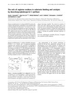
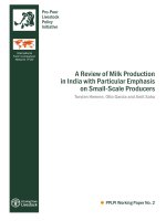
played in Fig. 1, Cho et al. (1998) by visual observations and acoustic
methods as shown in Fig. 2 and by Aya and Nariai (1991). Also, notice
that the lines of Fig. 1 separating the different condensation regimes can
change with the sparger or nozzle diameter. However, these changes are
not very pronounced, as observed by Song and Kim (2011).
In general, these maps contain six regions: the chugging region

denoted by (C), which occurs at relatively low steam mass flux and high
subcooling. In this region, steam bubbles are formed outside the injec­
tion pipe and collapse periodically, and therefore, the water from the
pool flows back entering the pipe exit region. Then, the pressure in­
creases in the pipe, and the steam exits again and forms bubbles that
collapse and the previous process is repeated. In the condensation os­
cillations region (CO), the interface oscillates violently, the steam con­
denses outside the nozzle, and the surrounding water moves back and
for following these oscillations. The TCO is the region of transition from
chugging to condensation oscillations, with the characteristic that the
subcooled water does not enter the nozzle. The SC region, which occurs
for higher steam mass flux and high subcooling, is the region where
stable condensation happens and only the jet end oscillates importantly.

There are two additional regions when the pool temperature rises above
80 ◦ C and is approximately below 92 ◦ C. The first one, below a mass flux
of 340 kg/m2s, is the BCO or bubbling condensation oscillation region,
where irregular bubbles detach from the discharge pipe, and then
condense or escape. The second one, above this max flux value, is the
IOC or interfacial oscillation condensation region characterized by the
non-stable character of the jet interface (Hong et al., 2012).
Norman et al. (2006) performed a detailed analysis and a set of ex­
periments on jet-plume condensation of steam-air mixture discharges in
a subcooled water pool. The objective was to study all the phenomena
that appear in the three regions of a buoyant gas jet: the momentum
dominated region, the transition region and the ascending plume
dominated by buoyancy forces, and in addition, the thermal response of
the pool. Norman et al. performed the study for different vent sizes,
different mass flow rates, different degrees of subcooling in the pool, and
finally, different mass fractions of non-condensable gases in the mixture.
Then Norman and Revankar (2010-a) and Norman and Revankar
(2010-b) completed this work with two papers on this same issue.
The discharges of mixtures of steam and NC gases as air has been
performed more recently by several authors as Qu and Tian (2016),
which have conducted experiments on condensation of a steam–NC
mixture jet discharged in the bottom of a subcooled water tank. They
observed that the momentum-dominated region becomes an ascending
plume formed by tiny bubbles after losing its initial momentum.
This paper’s main goal is to study and deeply analyze the jet
condensation-oscillations produced by the discharges of a steam flow
into a subcooled pool. First, it has been reviewed the works of Fukuda
(1982) , Fukuda and Saitoh (1982) and Aya et al. (1980, 1986, 1991),
extending these studies to ellipsoidal condensing-jet shapes, considering
recent advances performed by authors as Villanueva et al. (2015), and

Gallego-Marcos et al. (2019) for the estimation of the average heat
transfer coefficient (HTC). Then, we study the capability of Fukuda and
Saitoh. models extended to hemi-spherical prolate steam jets to predict
the subcooling threshold for the transition and condensation oscillation
regimes when incorporating Gallego-Marcos et al. correlation for the
HTC. In addition, it is performed a comparison of these model pre­
dictions with the experimental data for low and high frequency pressure
oscillations. Furthermore, this paper also studies the instabilities pro­
duced in the SC and IOC regimes, calculating the frequency predictions
with different models, and comparing the results with Hong et al.’s
(2012) experimental data.
The organization of the paper is as follows: first, in section 2 we have
reviewed, the direct contact condensation heat transfer and the pene­
tration length of a steam jet discharged into a subcooled pool. Then we
have used these analyses as support for section 3. In sections 3.1, 3.2,
and 3.3 we have performed a revision of the oscillations of discharged
steam jets into subcooled water pools in the following map regions:
transition condensation (TCO), condensation oscillation (CO), and
bubbling condensation oscillation (BCO). Then, in section (3.4) we have
conducted the study of the oscillations in the stable condensation (SC)
and the interfacial oscillation condensation (IOC) map regions. Finally,
in section 4, we have discussed the main conclusions and new research
areas of interest in this field.

Fig. 1. Regime map for direct contact condensation obtained by Chan and
Lee (1982).
2


J.L. Mu˜

noz-Cobo et al.

Progress in Nuclear Energy 153 (2022) 104404

Fig. 2. Condensation regime map for direct contact condensation (DCC) according to Cho et al. (1998).

2. Fundamentals of direct contact condensation heat transfer
and jet penetration length
2.1. Direct contact condensation heat transfer

f̂ (p) = 5.9083 10−

e

molecular weight of the steam, R is the gas constant. In addition, pv is the
vapor pressure, Tv is the vapor temperature, pl is the liquid pressure and
Tl the liquid temperature, and hfg is the specific enthalpy of phase
R
change. The standard value of M
= 462 kgJ◦ K for pure steam is used, and

2RT
M

Γ(a) ≈ 1 +

πa = 1 +

q′′i
√̅̅̅̅̅̅

π
hfg ϱv 2RT
M

(6)

(7)

Another common formula to express equation (5) is to consider pv =
( R)
( R)
kB
R
Tv , pl = ρsat
v (Tl ) M Tl , and M = m , being kB the Boltzmann constant
M
and m the mass of a molecule of steam. In this case, equation (5) is also
usually expressed in the form:
[ ̂ ] (
)1/2 (
)
2f
kB
q′′i =
hfg
(8)
ρv Tv1/2 − ρvsat (Tl )Tl1/2
̂
2
π

m
2− f

(2)

Chandra and Keblinski (2020) used molecular dynamics to obtain the
accommodation coefficient f̂ . They obtained that the accommodation
coefficients depend on the liquid temperature near the interface, and
they provide the following law that fit well their results and the previ­
ously calculated ones by other authors:

(3)

√̅̅̅

1.3686

ρv

f̂ (Tl ) = − 4.16 10− 6 (Tl )2 + 2.15 10− 3 Tl + 0.73

(9)

Also, Labuntsov, and Muratova and Labuntsov (Kryukov et al., 2013)
have solved the Boltzmann kinetic equation for weak evaporation and
condensation, deducing more accurate formulas than equation (5) for
non-equilibrium condensation and evaporation processes, in this case,
they found:

For high-temperature condensing processes like the one for water

steam, the value of a is normally small; for instance, for a heat
condensing flow of 100 kw/m2 , the value of a is 1.3 10− 4 , but when the
condensation mass flux increases, then the value of a also increases. For
small values of a, Γ(a) can be approximated by the expression (Carey
1992):
√̅̅̅

( )−
p
p0

vv (p)
f̂ (p) = 0.05
vv (p0 )

Being erf(a) the mathematical error function. The physical meaning
of Γ(a) is that this coefficient, according to Collier (1981), results from
the net motion of the steam toward the interface and this motion is
superimposed on the motion produced by the Maxwell distribution. The
expression for a is given by the ratio of the steam velocity component w,
normal to the interface that is produced by the steam condensation and
the characteristic molecular steam velocity in kinetic theory:
q′′i
√̅̅̅̅̅̅
hfg ϱv 2RT
M

3

Being p0 a reference pressure that is taken equal to 1 bar, this effect is

a consequence of considering the gas as a real gas. In addition, Komnos
(1981) considers the deviation in the gas behavior from that of an ideal
gas and obtained for the accommodation coefficient the following cor­
relation based on the specific volume of the steam:

Where ̂f c is known as the accommodation coefficient for condensation
while, ̂f is the accommodation coefficient for evaporation, M is the

w
a = √̅̅̅̅̅̅ =

(5)

Several efforts have been conducted to obtain the accommodation
coefficient. Marek and Straub (2001) performed a fitting to the data of
Finkelstein and Tamir (1976) and obtained the following expression for
f̂ , which diminish when the pressure increases:

The first theories on direct contact condensation were based on ki­
netic theory, Schrage (1953) conducted a theoretical study on the
interphase heat transfer and deduced, based on kinetic theory, expres­
sions for the net mass flux m′′i and the net heat flux q′′i condensing at the
interface and which are given by:
)
(
)1/2 (
M
̂f c Γ(a)pv − ̂f e pl
q′′i = hfg m′′i = hfg
(1)

2πR
Tv1/2
Tl1/2

finally, Γ(a) is given by the expression:
( )
√̅̅̅
Γ(a) = exp a2 + a π(1 + erf(a))

)
] (
)1/2 (
2̂f
M
pv
pl
hfg
−
1/2
1/2
2πR
2 − ̂f
Tv
Tl

[
q′′i =

[
q′′i =

(4)

] (
)1/2 (
)
kB
hfg
ρv Tv1/2 − ρvsat (Tl )Tl1/2
̂
2πm
2 − 0.798 f
2̂f

(10)

Expression (10) is helpful to obtain upper limits for the direct contact
condensation heat flux.

Substituting the value of Γ(a) given by expression (4), in equation
(1), and clearing q′′i , yields the expression obtained by Silver and
Simpson (1961) and if the accommodation coefficients for evaporation
and condensation have the same value:
3


J.L. Mu˜
noz-Cobo et al.

Progress in Nuclear Energy 153 (2022) 104404

2.2. Jet penetration length for discharges of pure steam

remaining effects in the value of the transport modulus.
Petrovic (2005), after performing a parametric study of the shape of
the steam plumes for different boundary conditions, arrived at the
conclusion that for conditions of high steam mass flux, high pool tem­
perature and small diameter of the injectors the shape of the steam
plume is ellipsoidal. Assuming an axisymmetric plume of length lp , as
displayed in Fig. 3a, the variation of the plume radius r(x) with the
distance is:
√̅̅̅̅̅̅̅̅̅̅̅̅̅
x2
r(x) = r0 1 − 2
(18)
lp

One of the first semi-empirical derivations of the jet penetration
length for a steam-jet discharging in a subcooled water pool was ob­
tained by Kerney et al. (1972). First, these authors deduced a semi­
empirical formula for the penetration length and then they improved
this expression by fitting the coefficients and exponents to the experi­
mental data. Denoting by h the local heat transfer coefficient from the
steam to the water, by Ws (x) = πr2 G(x) the steam mass flow rate at the
axial position x, and by m′′c (x), the condensation mass flux at the inter­
face, then the change of the steam mass flow rate along x is given by the
equation:
d
W(x) = − 2πrm′′c (x)
dx

withm′′c (x)hfg

= h(Ts − T∞ )

Because of the element of the interfacial area dS =
√̅̅̅̅̅̅̅̅̅̅̅̅̅̅̅̅̅̅̅̅̅̅̅̅
2πr(x) 1 + (r′ (x))2 dxfor direct contact condensation changes with the

(11)

distance, then the expression for the mass flow rate change is given
instead of equation (11) by:
√̅̅̅̅̅̅̅̅̅̅̅̅̅̅̅̅̅̅̅̅̅̅̅ ′′
dWs (x) = − 2πr(x) 1 + (r′ (x))2 mc dx =
√̅̅̅̅̅̅̅̅̅̅̅̅̅̅̅̅̅̅̅̅̅̅̅
h(Ts − T∞ )
− 2π r(x) 1 + (r′ (x))2
dx
(19)
hfg

Equation (11) can be written after some calculus because of the ex­
pressions for m′′c (x) and W(x) and after dividing by the mass flow rate W0
at the nozzle exit in the form:
(
)1/2
( )12
d Ws (x+ )
G

=
−
Sm B
dx+ Ws,0
G0

(12)

Integrating expression (19) between x = 0,Ws (0) = Ws,0 , and x = lp ,
with Ws (lp ) = 0 yields for the case of an ellipsoidal steam plume:
∫ lp
√̅̅̅̅̅̅̅̅̅̅̅̅̅̅̅̅̅̅̅̅̅̅̅
hΔT
hΔT
Ws,0 =
(20)
Ai =
2π
r(x) 1 + (r′ (x))2 dx
hfg
hfg
0

Where x+ = x/r0 , is the dimensionless axial distance, B is the conden­
sation driving potential defined by the expression
B=

cp (Ts − T∞ )
hfg

(13)

Being Ai the interfacial area between the steam and liquid phases, h
the average heat transfer coefficient.
After some calculus it is obtained assuming that r(x) is given by
equation (18) the following result:
⎧
)1/2
(
)1/2 ⎫
(
⎬
hΔT
π r0 lp ⎨
r02
r0
r02
1
−
Ws,0 =
arcsin
1
−
(21)
+
(
)
1/2
2
2

⎩
⎭
hfg
r2
lp
lp
lp
1 − l20

Being Ts the saturation temperature and T∞ the bulk temperature of
the pool. Finally, Sm is a nondimensional number analogous to the
Stanton number, and defined for this case as follows:
Sm =

h
cp G

(14)

Equation (12) can be integrated with the boundary conditions at the
nozzle exit and at the penetration length lp of the jet where all the steam
is condensed, so it is obtained:
Ws
Ws
lp
= 1 at x+ = 0, and
= 0 at x+ =
Ws,0
Ws,0
r0

p

If the injector exit radius r0 is much smaller than the steam penetra­
tion length lp , i.e., r0 ≪lp , then equation (21) can be approximated
retaining only first-order terms in rlp0 :

(15)

To integrate equation (12), it is necessary to know how G(x+ )
changes with x+ , and Sm with x+ . Assuming some average values Gm for
G and Sm for Sm , the integration of (12) yields for the dimensionless
steam penetration length Xp the following result deduced by Kerney et al.
(1972):
Xp =

2lp
− 1
= S m B−
D0

(
1

G0
Gm

)1/2

Ws,0 =

(16)

from equation (22), it is deduced the following expression for the
dimensionless penetration length:
(
( )
}
)
{
lp 2lp 2 G0 hfg
− 1 G0
Xp = =
=
− 1
(24)
− 1 = 0.6366 B− 1 Sm
r0 D0 π hΔT
Gm
Where B is the condensation driving potential, Sm is the average Stanton
number and Gm the average mass flux. So, it has been obtained again
that the penetration length depends on the inverse of the driving po­
( )
− 1
tential B− 1 , the inverse of the average Stanton number Sm and GGm0 .

experiments were in the range 332 − 2044 mkg2 s, the bulk temperature of the
pool denoted by T∞ was in the range 301 − 352 K at atmospheric pres­
sure, the condensation driving potential B was in the range 0.0473 −
0.1342. Then, Kerney et al. performed a fit to their data in terms of B and

( )
G0
, obtaining that the expression that best fit the data was:
Gm
2lp
= 0.7166 B−
D0

(
0.8411

G0
Gm

)0.6466

(22)

Consequently, when r0 ≪lp the interfacial area can be approximated
up to first order by:
{
}
π r0
Ai = πr0 lp
(23)
+
2 lp

Kerney et al. chose for Gm the value of 275 kg/m2s because the data
of their experiments were obtained with choked injector flows and the

remaining effects were included in the transport modulus Sm , which is
obtained experimentally. The 128 experiments performed by these au­
thors cover an extensive range of boundary conditions, the injector di­
ameters D0 were in the range 0.0004 − 0.0095 m, the mass fluxes G of the

Xp =

{
}
hΔT
π r
πr0 lp + 0
hfg
2 lp

Also, equation (24) shows that the penetration length increases with the
initial mass flux, while diminishing with the DCC heat-transfer coeffi­
cient and with the pool subcooling.
An expression for the Stanton number is first needed to obtain the
penetration length from equation (16) or (24). Several authors as Kim
et al. (2001), Chun et al. (1996), Gulawani et al. (2006), and Wu et al.
(2007) have obtained correlations for the average HTC, all of them can
be expressed in terms of the Stanton number, as displayed in Table 1, the
correlations were obtained using different exit nozzle diameters (D0 ).

(17)

Also, these authors give an expression based on equation (16), using
the assumption of Linehan and Grolmes (1970) that a constant transport
modulus Sm , provides a reasonable correlation and includes all the

4


Progress in Nuclear Energy 153 (2022) 104404

J.L. Mu˜
noz-Cobo et al.

Fig. 3. Discharge of a) a hemi-ellipsoidal prolate jet and b) an ellipsoidal steam jet into a subcooled pool, both with steam penetration length lp .

(

Table 1
Correlations for the transport modulus (Stanton number) of different authors for
the discharge of steam jets in a subcooled pool.
Method

Correlation

Average
HTC

h
=
cp Gcrit

Kim et al. (2001)
(

G0

Gcrit

)0.13315

D0 = 5mm, 7.1mm, 10.15mm,
15.5mm, 20mm

Average
HTC

( )0.3714
h
G0
= 1.3583B0.0405
cp Gm
Gm

Chun et al. (1996)

Average
HTC

(
)
h
G0 1.31
= 1.12B0.06
cp Gcrit
Gcrit
(

)
h
G0 1.12
= 1.54B0.04
cp Gcrit
Gcrit
(
) ( )0.2
pf
h
G0
= 0.576B0.04
Gcrit
ps
cp Gcrit

Gulawani et al. 2006
D0 > 6mm

Average
HTC

D0 = 1.35 mm, 4.45 mm,
7.65 mm,
10.85 mm.
Gulawani et al. 2006
D0 < 2mm

Wu et al. (2007)

D0 = 2.2 mm, 3mm

(
Xp = 0.4686 B−

1.0405

G0
Gm

are:

)0.6286
− 0.6366

)0.3665

(26)

Where N is the number of experimental points, p the number of fitting
parameters, yth,i denote the theoretical values obtained with the corre­
lation, and yexp,i the experimental values.
The results obtained for the RMSE with the different correlation and
semiempirical formulas show us that the expressions based on equation
(27) generally have a little bit less RMSE error than the expressions
based on the Kerney type equation.

ney’s equation is used for Xp and Kim’s correlation for Sm , or ellipsoidalChun if equation (24) is used, assuming an ellipsoidal shape for the jet
and Chun’s correlation for the Stanton number. The expressions ob­
tained for Ellipsoidal-Chun and Kerney-Kim for the dimensionless

2lp
D0

G0
Gm

The fitting parameter values bi of equation (27) have been obtained
with the non-linear fitting program nlfit of MATLAB, using the 104
experimental data of Kerney for different diameters of the nozzle and
different boundary conditions, the values of these fitting parameters are
displayed in Table 2. Also, the experimental data of Kerney using the
nlfit routine of MATLAB have been refitted obtaining a new correlation
with smaller root mean square error (RMSE). Additionally, this table
shows in the last column the RMSE error, which is used as a merit figure
to compare the different correlations and semiempirical formulas:
√̅̅̅̅̅̅̅̅̅̅̅̅̅̅̅̅̅̅̅̅̅̅̅̅̅̅̅̅̅̅̅̅̅̅
√∑
)2
√N (
√
y − yexp,i
√i=1 th,i
RMSE =
(28)
N− p

Substituting the expressions for the Stanton number into Kerney’s
expression, equation (16), or equation (24) for the ellipsoidal jet, one
obtains a set of semi-empirical expressions for the dimensionless pene­
tration length (Xp ). Expression which is denoted as Kerney-Kim, if Ker­

penetration lengths Xp =

1.03587

Expression (25) provides an alternative correlation expression to
Kerney’s form, given by equation (17), which can be expressed as:
( )b 3
G0
Xp = b1 B− b2
− b4
(27)
Gm

References

1.4453 B0.03587

Average
HTC

Xp = 0.692 B−

2.3. Condensation heat transfer coefficients (HTC) for steam jets

(25)

Fukuda (1982), and Simpson and Chan (1982) investigated the

Table 2

Comparison of different correlations and semiempirical formulas for Xp using Kerney Experimental data set and Gcrit = 275
Name

Method

Kerney Method

Kerney original equation

Xp =

(

KerneyEllipsoidal

Expression from ellipsoidal jet shape and fitted coefficients from Kerney-data

EllipsoidalChun

Integration of the mass conservation equation assuming ellipsoidal jet form and Chun et al.
correlation for the transport modulus

Kerney-Kim

Expression of Kerney with Kim et al. correlation for the transport modulus

(1997)

Kim et al.

0.8411

G0
Gcrit

(

Kerney data refitted with the nlfit program of MATLAB

Kim et al.

RMSE

2lp
D0

0.7166 B−

Kerney- refitted

kg
.
m2 s

)0.6466

2.6499

)0.6785

2.5816

G0
0.8463 B
Gcrit
(
)
G0 0.5521
1.7692 B− 0.6309
−
Gcrit
3.4663
( )0.6286
G0
0.4686 B− 1.0405
−
Gm
0.6366
( )0.3665
G0
0.692 B− 1.03587
Gm
( )0.344
G0
1.1846 B− 0.66
Gm
− 0.7671

Expression of Kim et al. for the pool at atmospheric pressure and Gm = 275kg/m2 s

(

Expression of Kim et al. for the dimensionless penetration length

1.06 B−

(2001)

5

0.70127

G0
Gm

)0.47688

References
Kerney et al.
(1972)

2.5777

3.5963

5.1778
6.176
4.337

Kim et al. (1997)

Kim et al. (2001)


J.L. Mu˜
noz-Cobo et al.

Progress in Nuclear Energy 153 (2022) 104404

interfacial heat transfer coefficient in DCC for steam discharges. They
estimated a time average value of the heat transfer considering that the
steam mass flow rate Ws into de bubble was constant and equal to the
existing one at the vent discharge i.e., Ws = πr02 Gs . In addition, Fukuda
computed the heat transfer coefficient at the maximum radius attained
by the bubble and assuming that the entering mass flow rate was equal
to the condensing mass flow rate at this maximum radius, which as was
obviously noticed by Gallego-Marcos et al. (2019) under-estimate the
heat transfer coefficient. This simple calculation yields:

π r02 Gs =

hΔT
π r2 Gs hfg
2
4πrmax
⟹h = 02
hfg
4π rmax ΔT

pool temperature increases the chugging oscillations occur at lower
mass fluxes. As mentioned in the introduction, in the chugging region,

the bubbles are formed outside the vent pipe and when attain a given
size break up and condense so the pool water flow back penetrating into
the vent discharging pipe (Wang et al., 2021). This process continues up
to a limit length where the pressure exerted by the steam flux coming
from the header pushes up all the liquid outside the vent, and the steam
penetrates again into the pool forming a new bubble that when attains
some size it breaks and collapses and the pool water again flows back to
the vent, starting a new cycle, which is repeated periodically. In the
transition region (TC), the oscillations are like the chugging ones except
that the amplitude of the oscillations is smaller, and the water does not
enter inside the vent line, and a cloud of small bubbles is formed near the
vent exit. The other oscillations studied in this section are the conden­
sation oscillations (CO) in these oscillations that take place at greater
mass fluxes, the steam condensation occurs outside the vent nozzle and
therefore the water does not enter inside the vent tube and the steam
water interface oscillates violently (Hong et al., 2012). Finally, if the
pool temperatures increase above 80 ◦ C appear the so-called bubbling
condensation oscillations (BCO) where the bubbles detach periodically
with some characteristic frequency.
Arinobu (1980), Fukuda and Saitoh (1982), Aya and Nariai (1986),
Zhao et al. (2016), Villanueva et al. (2015), Gallego-Marcos et al. (2019)
performed several sets of experiments covering the following conditions:
chugging (C), the transition to condensation oscillations (TC), the
condensation oscillations (CO) and the bubbling (BCO). They also per­
formed experiments to try to predict the temperature subcooling
thresholds for the appearance of the low frequency and the high fre­
quency oscillations. They found experimentally (Aya and Nariai 1986)
that for high frequency oscillations the temperature-subcooling
threshold ΔTTHf disminishes with the mass flux, however for
low-frequency oscillations Arinobu (1980) found that the temperature

subcooling threshold ΔTTLf was practically constant with the steam mass
flux.
In this section, the models of Fukuda and Saitoh (1982) and Aya and
Nariai (1986) are reviewed, but instead of a spherical or a cylindrical
model an ellipsoidal jet model has been used. Additionally, a compari­
son of the new results with these of previous models and with the
experimental data has been carried out, also discussing the best way to
improve their predictions. Finally, it has been found that especially
useful to improve the results are the correlations obtained by Gallego-­
Marcos et al. (2019).
A model like the one used by Aya and Nariai (1986) is considered,
but with a prolate hemi-ellipsoidal shape for the steam-jet. The steam
bubble is assumed to have an ellipsoidal shape, as displayed at Fig. 4,

(29)

Then Fukuda measured the maximum radius with a high-speed
camera and proposed the following correlation for the Nusselt number:
)0.9
(
hdv
dv Gs
cp,l ΔT
Nu =
= 43.78
(30)
hfg
kl
μl
Where ΔT = Ts − T∞ , is the subcooling and the rest of the symbols are

standard ones. Then Simpson and Chan (1982) performed the calcula­
tion of h performing an average of the interfacial area over a complete
cycle of the bubble.
Gallego-Marcos et al. (2019) computed the heat transfer considering
that during the time interval Δt, the spheroidal bubble size increases its
volume ΔVelip and therefore a portion of the incoming mass ρs ΔVelip does
not condense during this time interval. After detachment, the neck re­
duces its diameter andΔVelip could become negative especially when
Qb = 0 i.e., when the bubble is completely detached. In general, the heat
transfer coefficient (HTC) can be obtained from the expression:
(
)
ρ Qb Δt − ΔVelip hfg
h= s
(31)
Ai,elip ΔT
where Qb is the volumetric flow rate in m3 /s, which is equal to the steam
volumetric flow rate Qs,inj = πr02 vs,inj injected at the vent exit before the
bubble detachment. After the detachment, Gallego-Marcos et al. (2019)
found that the neck connecting the vent exit to the steam bubble was
varying its size leading to a significant uncertainty in the determination
of the volumetric flow rate Qb to the steam. Therefore Gallego-Marcos
et al. (2019) computed the HTC only for the detachment phase, and the
correlation obtained for the Nusselt number is given by the expression:
Nu =

h dv
−
= 5.5 Ja0.41 Re0.8
s We

kl

0.11

(32)

where Ja is the Jakob non-dimensional number, Re the Reynolds num­
ber and We the Webber number. The definitions used for these numbers
in equation (32) are:
Ja =

cp,l ΔT
Gs dv
ρ u2 d
, Re =
, We = s s
hfg
μs
σ

(33)

Several authors have investigated the interfacial heat transfer coef­
ficient in DCC during steam jet discharges, Chun et al. (1996) obtained
that the average HTC depends on the steam mass flux G and the degree
of pool subcooling ΔTsub = Tsat − Tl , increasing with G. These authors
found that the average HTC, hm was in the range of 1.0–3.5 mMW
2K .
Otherwise, Kim et al. (2001) found that the average HTC was in the
interval 1.24–2.05 mMW

2 K. More information on the average heat transfer
coefficient hhas been shown in Table 1.

3. Oscillations of discharged steam jets in subcooled water pools
3.1. Transition and condensation oscillations
Fig. 4. Model for the discharge of a steam mass flow rate into a pool a tem­
perature Tl thought a discharge pipe or vent of diameter dv = 2r0 , assuming a
hemi-ellipsoidal shape for the steam discharge.

The chugging oscillations (C), as displayed at Figs. 1 and 2, appear
for low steam mass fluxes G and low pool water temperatures, and as the
6


J.L. Mu˜
noz-Cobo et al.

Progress in Nuclear Energy 153 (2022) 104404

with penetration length lp (t) that oscillates around the value ls , being z(t)
the variation with time of the length of the oscillations around the
average penetration value, so it can be written:

(
) 2
1
d z
δps = ρl lm + (ls + z(t))
3
dt2

Therefore, the pressure change with time is governed by the
equation:
) 3
(
dps dδps
1
d z(t)
1 dz d2 z
+ ρl
(45)
=
= ρl lm + (ls + z(t))
3
dt3
3 dt dt2
dt
dt

(34)

lp (t) = ls + z(t)

Where according to Fig. 4 z(t) can be positive or negative. It is assumed
that the inertial effect of the pool water against the interfacial motion is
represented by all the water contained inside the cylinder of length lm ,
plus the amount of water contained in the volume of the cylinder of
length lp minus the volume of the hemi-ellipsoid as displayed at Fig. 4.
For small mass fluxes, the steam does not penetrate too much, and
the shape of the bubble is spherical as assumed by Fukuda and Saitoh

(1982) or conical. For bigger jet lengths, it can be assumed to have cy­
lindrical or hemi-ellipsoidal shapes.
The mass conservation equation for the steam volume Vs can be
written as follows:
d
π
hΔT
(Vs (t)ρs ) = dv2 Gs −
Ai (t)
dt
hfg
4

The oscillations in lp (t)take place around the equilibrium value ls ,
and at equilibrium conditions, equation (38) reduces to:
(
)
π 2
hΔT0
π
hΔT0 π2
Ai,o = dv2 Gs −
(46)
dv Gs −
r0 ls + πr02 = 0
4
hfg
4
hfg
2

Subtracting equation (46) from equation (38) yields because of
equation (40):
d
dt

ρs Vs (t) + Vs (t)

(35)

Ai (t) ≅

π

2

2

r0 lp (t) + πr02

d3 z
d2 z
dz
+ A 2 + B + C z + non − linear terms = 0
dt3
dt
dt

(36)

d

dt

∂ρs dps π 2
hΔT
Ai (t)
= dv Gs −
hfg
∂ps dt
4

(37)

Assuming that the oscillations of the physical magnitudes are per­
formed around an equilibrium value denoted by the subindex 0, then
one may write:
(39)

ΔT = Ts (t) − Tl = ΔT0 + δΔT(t) = ΔT0 + δTs (t)

(40)

∂Ts
δp
∂ps s

(41)

d2 z
dt2

(42)

where the inertial volume displayed at Fig. 4 in dark blue color is given
by the expression:
1
Vinertia = πr02 lm + π r02 lp (t)
3

2
πr02
ρs
∂p
3
(
)(
) s
2
2
ρl V0 + 3 πr0 ls lm + 13ls ∂ρs

(50)

C=

hΔT0
π 2 r0
∂p
(
)(
) s

hfg ρl V0 + 23 πr02 ls lm + 13ls ∂ρs

(51)

Because of the general solution of equation (52) can be obtained by a
linear superposition of 3 linearly independent solutions if the matrix [J]
has three linearly independent eigenvectors v(j) . Then the general solu­
tion of the linear problem can be expressed in the form (Guckenheimer
and Holmes 1986):

The fluctuation in δps are governed considering the Newton law and
the inertial mass displayed at Fig. 4, by the equation:

π r02 δps = ρl Vinertia

B=

Considering that the system stability is determined by the Lyapunov
exponents of the linear part (Guckenheimer and Holmes 1986), which
are the eigenvalues of the Jacobian Matrix of the system at the equi­
librium point, which are obtained as it is well known by solving the
equation:
⃒
⃒
⃒0 − λ
1
0 ⃒⃒
⃒
⃒ 0
0− λ

1 ⃒⃒ = 0⇒λ3 + Aλ2 + Bλ + C = 0
(53)
⃒
⃒ − C
− B A − λ⃒

The fluctuations in the difference of temperature between the steam
and the liquid pool are related to the fluctuations of temperature of the
steam and are given by:
δTs =

(48)

Equation (48) can be converted to a non-linear ordinary differential
equation system, by performing the changes of variables z˙ = z1 , z˙1 = z2 ,
the linear part of this ordinary differential equation system is:
⎞⎛ ⎞
⎛ ⎞
⎛ ⎞ ⎛
0
1 0
z
z
z
d⎝ ⎠ ⎝
0
0 1 ⎠⎝ z1 ⎠ = [J]⎝ z1 ⎠
(52)
z1 =
dt

− C − B A
z2
z2
z2

(38)

ps (t) = ps,0 + δps (t)

(47)

The coefficients of the linear terms in equation (48) are given by:
(
)
( )
( )
π2
2
h 2 r0 ls + πr0
∂Ts
h Ai,0 ∂Ts
(
)
A=
=
(49)
2
2
hfg V0 + 3 πr0 ls
hfg Vs,0 ∂ρs

∂ρs

The volume V0 in equation (36) is the volume of the header VD plus
the volume of the vent tube, the second term is the volume of a half
prolate-spheroid. The interfacial area expression has been obtained from
equation (23).
If the steam is at saturated conditions or close to them then ρs = ρs (p)
and on account that the pressure changes with time, then operating in
equation (35) yields:

ρs Vs (t) + Vs (t)

∂ρs dps
hΔT0 π 2
h δΔT
Ai (t)
=−
r0 z(t) −
hfg
∂ps dt
hfg 2

Then considering equations (41) and (44)–(46), in equation (47) it is
obtained after some calculus and algebra the following equation for the
evolution of z(t), where only the linear terms in z(t) and their derivatives
are explicitly displayed:

Where Vs (t) is the steam volume, and Ai (t) denotes the interfacial area of
the steam with the surrounding liquid. The expression for both magni­
tudes can be written in terms of the penetration length lp (t) of the jet in

the water pool as:
2
Vs (t) = V0 + πr02 lp (t)
3

(44)

3
∑

z(t) =

cj v(j) eλj t

(54)

j=1

(43)

Therefore, the linear system is stable is Re λj < 0 , j = 1, 2, 3, and
unstable if Re λj > 0for j = 1, 2, 3. By the Hartman-Grobman theorem
˜ oz-Cobo and Verdú, 1991), the
(Guckenheimer and Holmes 1986, Mun
system stability can be extended to the entire system including the

From equations (42) and (43), it is obtained after some
simplifications:

7

Progress in Nuclear Energy 153 (2022) 104404

J.L. Mu˜
noz-Cobo et al.

non-linear part, with the condition that the real parts of all the eigen­
values of the Jacobian Matrix [J] at the equilibrium point are ∕
= 0.
The system stability can be obtained by applying the Routh Hurwitz
criterium to the characteristic equation (53) (D’Azzo and Houpis, 1988).
Application of this criterium yields:
⃒
1
B
λ3 ⃒⃒
2⃒
A
C
λ ⃒
(55)
λ1 ⃒⃒ (AB − C)/A .
0⃒
C
.
λ

Table 3
Subcooling threshold for low and high frequency oscillations in discharges of

steam in subcooled pools.

To be stable, the sign of all the terms of the first column must be the
same, in this case positive therefore, A > 0, C > 0 and AB > C, therefore
for stability it also follows that B > 0. Therefore, the threshold for sta­
bility is given according to this criterium by the condition:

ls + dπv ∂Ts
ρ
ls + Vd02 s ∂ρs
π

Spherical

Spherical
Cylindrical

Subcooling
Threshold
ΔTTLf =
2πr3
∂T
ρ s
4 3 s ∂ρs
V0 + πr
3
3 ∂T s
ΔTTHf = ρs
2 ∂ρs
ΔTTLf =

ls +
ls + (

(57)

v
6

ls + dπv ∂Ts
ρ
ls s ∂ρs

Aya-and Nariai-High
frequency oscillations

Cylindrical

This paper-Low frequency
oscillations

Hemi-ellipsoidal
(Spheroid-prolate)

This paper-High frequency
oscillations

ΔTTHf =

ls +

ls

dv
4 ρ ∂T s
s

∂ρs

ΔTTLf =

dv
π ρ ∂T s
V0 s ∂ρs
ls + 2
d
π v
6

Hemi-ellipsoidal
(Spheroid-prolate)

ΔTTHf =

ls +
ls

dv

π ρ ∂T s
s

∂ρs

3.2. Results for the transition (TCO), condensation oscillations (CO), and
bubbling condensation oscillations (BCO)

Fukuda (1982) and Aya and Nariai (1986) obtained expressions for
the subcooling thresholds, which are shown in Table 3.
To obtain the subcooling threshold with the different models, it is
needed to compute two magnitudes the first one is the partial derivative
∂Ts
∂Ts
∂ρ and the second one the steam penetration length. To compute ∂ρ , it is

Experimental data for the subcooling threshold for high frequency
oscillations ΔTTHf with different mass fluxes were obtained by Fukuda
and Saitoh (1982) and by Aya and Nariai (1986). The results for this
case, as shown in Table 3, depends on the penetration length ls , the vent
diameter dv , and the product of the steam density and the partial de­
rivative ∂∂ρTs , which for polytropic processes, because of equation (59),

s

assumed that the process is polytropic because most of the thermody­
namic process of practical interest are polytropic with coefficient n
varying between 1 ≤ n ≤ 1.3 for water steam. For a polytropic process it
holds:
( )n− 1
1
∂Ts
Ts

Ts
= cte⇒
= (n − 1)
(59)

∂ρs

πd2v

∂T
ρs s
) ∂ρs

ls +

(58)

s

dv
4
V0
4

Pressure oscillations of low frequency start when the water pool
subcooling ΔT exceeds the threshold subcooling given by equation (57).
Low and high frequency pressure-oscillations can exist, according to Aya
and Nariai (1986), the lower ones are controlled by the steam volume of
the header plus the vent and the volume of the jet-steam i.e. V0 + 23 π r02 ls ,
while the high frequency pressure oscillations are controlled only by the

steam jet volume23 πr02 ls .
The threshold subcooling for high frequency oscillations is obtained
by setting V0 = 0 in equation (57) that yields:

ρs

Fukuda-low frequency
oscillations

Fukuda-high frequency
oscillations
Aya-and Nariai-low frequency
oscillations

From equation (56) because of equations (49)–(51), it is obtained
after some simplifications the following expression for the subcooling at
the oscillation threshold when the jet shape is hemi-ellipsoidal as dis­
played at Fig. 3:

ΔTTHf =

Jet Shape

(56)

AB = C

ΔTTLf =

Name

s

depends on the polytropic exponent n. Also to obtain ls , because of
equation (60), it is necessary to know the average heat transfer coeffi­
cient. These experiments clearly show as displayed in Fig. 5 that the
subcooling thresholdΔTTHf diminish with the steam mass flux Gs .
However, using the correlation obtained by Fukuda (1982), the result is
that ΔTTHf is practically constant.
If the correlation for the Nusselt number deduced by Gallego-Marcos
et al. (2019) and given by equation (32) is used, instead of the corre­
lation used by Fukuda and Saitoh (1982). First, it is observed that the
Gallego-Marcos et al. correlation depends on the subcooling and second
the expression (60) used to obtain the penetration length depends also

ρs

For polytropic processes with wet steam that suffer expansions and
contractions the polytropic index is ranging in the interval 1.08 ≤ n ≤ 1.2
depending on the characteristics of the process (Soh and Karimi 1996;
Romanelli et al., 2012), we have chosen the values of n = 1.07, 1.082,
1.09 to perform the calculations. For high temperatures of the liquid,
close to 90 ◦ C, when the steam condensation diminishes the polytropic
coefficient approach to 1.3.
To obtain the steam penetration length ls , it is performed a mass
balance between the injected mass flow rate and the condensed mass
flow rate, which yields for the spheroid-prolate case:
(
)
(

)
hΔT
hΔT π2
dv Gs hfg
π r02 Gs =
Ai =
r0 ls + πr02 ⇒ls =
− 1
(60)
hfg
hfg
2
π hΔT

on the subcooling and h, therefore the resulting equation is a non-linear
algebraic equation in ΔT, of the standard form x = f(x) and given by:
[
]
C1 kl (Tl )ΔT 1.41
∂T
ΔT = 1 +
ρs s
(61)
1.41
Gs hfg − C1 kl (Tl )ΔT
∂ρs
Where the coefficient C1 is given by:
( )0.41
5.5 cpl
− 0.11

C1 =
Re0.8
s We
dv hfg

To compute h in equation (60) we have used the HTC deduced from
Gallego-Marcos et al. (2019) correlation for the Nusselt number, and
which is given by equation (32).

(62)

The algebraic equation (61) has been solved by iterations, normally
8


J.L. Mu˜
noz-Cobo et al.

Progress in Nuclear Energy 153 (2022) 104404

Fig. 6. Subcooling threshold ΔTTHf for the high-frequency oscillations
computed using equation (61), and the correlation of Gallego-Marcos et al.
(2019), n = 1.082, and three vent diameters dv = 14, 16, 22 mm. Comparison
with the experimental data of Fukuda (1982) and Aya and Nariai (1986).

Fig. 5. Subcooling threshold ΔTTHf for high-frequency oscillations computed
using equation (61), with the correlation of Gallego-Marcos et al. (2019), three
values n = 1.077, 1.082, 1.085of the polytropic coefficient and dv = 16 mm.
Comparison with the experimental data of Fukuda (1982) and Aya and Nar­
iai (1986).

(1986). As was discussed by different authors as, Aya and Nariai (1986),
the low frequency components of the oscillations is controlled by a
larger steam volume, which includes the header and the section of pipe
from the header to the discharge vent, in the case of the experiments
performed by Chan and Lee (1982) the header volume was 0.044 m3 , in
the case of Aya and Nariai this volume ranges from 0.005 to 0.04 m3 . The
equation used to predict the subcooling threshold for low frequency
oscillations is equation (57), substituting in this equation the expression
for the penetration length given by equation (60) and because of the
expression for the heat transfer coefficient obtained by Gallego-Marcos
et al. (2019), given by equation (32), it is obtained after some calculus
the following equation for the low frequency subcooling threshold
denoted by ΔTTLf :
(
)
(
)
6V0
∂Ts
ΔT 2.41
F ΔTTLf = C2
=0
(64)
TLf + Gs hfg ΔTTLf − Gs hfg ρs
dv3
∂ρs

few iterations are needed for convergence, usually less than 10. In some
cases, particularly for low mass flux values smaller than 5 kg/ m2 s, the

Newton method has been used, since gives better convergence. Also, it is
noticed that the subcooling values obtained when varying the mass flux
are dependent on the polytropic coefficient n. Fig. 5 displays the high
frequency subcooling threshold computed with three different values n
= 1.077, n = 1.082 and = 1.085 of this coefficient, and with a vent
diameter dv = 16 mm. Also, notice that it has been observed that for all
these values of the polytropic coefficient, the calculated subcooling
thresholds are located between the experimental values obtained by Aya
and Nariai and those obtained by Fukuda. However, for n = 1.085 there
is one point that is a little bit above the experimental data, as displayed
at Fig. 5.
Because of Fukuda and Saitosh’s expression for the subcooling
threshold ΔTHfT is independent on the steam mass flux Gs , as it is
deduced considering Table 3. We have deduced that the polytropic
exponent used by Aya and Nariai (1986) to predict a threshold value of
ΔTTHf = 44.3 Kusing Fukuda expression is:
3
ΔTTHf = 44.3 = (n − 1)Ts ⟹n = 1.079
2

Where C2 is given by:
( )0.41
5.5kl cpl
−
C2 = C1 kl =
Re0.8
s We
dv hfg

(63)

0.11

(65)

Equation (64) has been solved by the following Newton iteration
algorithm that converges very fast for the analyzed cases:
)
(
F ΔTTLf
(r)
(
)
ΔT (r+1)
(66)
TLf = ΔT TLf −
′
F ΔTTLf

So, the polytropic coefficient is close to 1.08, and with this coeffi­
cient the model predictions given by equation (61) are close and a little
bit below the curve denoted as n = 1.082 in Fig. 5.
Also, from Fig. 5 it is observed that the subcooling threshold pre­
dicted by equation (61) diminish with the mass flux Gs as observed
experimentally. However, for high mass fluxes the slope of the curve
becomes smaller than the experimental one and for small mass fluxes
becomes bigger.
The results for the predicted subcooling threshold depend slightly on
the vent diameter, we have performed the calculations with three
different diameters dv = 12 mm, dv = 16 mm and dv = 22 mm, and the

results are displayed at Fig. 6. These results are also compared with the
experimental data of Fukuda and Aya and Nariai. It is observed that the
model predicts that the subcooling threshold diminishes when the vent
diameter increases.
Next, the liquid temperature threshold for the occurrence of low
frequency oscillation components in the discharges of steam into a
subcooled water pool will be discussed. Experimentally this case has
been studied by Arinobu (1980), Chan and Lee (1982), Aya and Nariai

Denoting by the supra-index r the subcooling result of the r-th iter­
′
ation and being F (ΔTTLf ) the derivative of the function F(ΔTTLf ), with
respect to the subcooling. For this case of low subcooling the polytropic
exponent should be closer to the adiabatic value of 1.3, and then this
value has been taken for the calculations. For the volume of the header
plus the pipes, a volume V0 = 0.04768m3 has been chosen, as suggested
by Lee and Chan (1980). In Fig. 7, it is represented the liquid temper­
ature threshold for low frequency oscillation versus the mass flux ob­
tained solving equation (64), with the previous data and a vent
discharge diameter of dv = 50.8 mm. It is observed that both curves are
very close and the variation of the slope with GS is practically the same.
It is convenient to analyze the sensitivity of the low frequency tem­
perature threshold Tl,TLf to the vent discharge diameter dv and to the
polytropic coefficient n. This threshold Tl,TLf was computed for three
9


J.L. Mu˜
noz-Cobo et al.

Progress in Nuclear Energy 153 (2022) 104404

Fig. 7. Liquid temperature thresholdTl,TLf = 100 − ΔTTLf for low frequency
pressure oscillations for steam condensation in pool water versus gas flux ac­
cording to Chan and Lee data (1982). The model results were calculated with
the facility data dv = 50.8 mm, V0 = 0.04768 m3 and a polytropic coefficient
value of n = 1.3.

Fig. 9. Liquid temperature thresholdTl,TLf for low frequency pressure oscilla­
tions for steam condensation in pool water versus the gas flux according to
Chan and Lee data (1982). The model results were calculated with three pol­
ytropic values n = 1.079, 1.2, 1.3, V0 = 0.04768 m3 and a vent diameter dv =
50.8 mm as in Chan and Lee experiment.

different vent diameters (dv = 45.8, 50.8, 55.8 mm) and three different
values of the polytropic coefficient (n = 1.079,1.2,1.3). In addition, these
results were compared with the experimental data of Chan and Lee
(1982).
Fig. 8 displays the results obtained solving equation (64) for different
vent diameters. It is observed that the experiment of Chan and Lee was
performed with a vent diameter of 50.8 mm, and the model results that
are closer to the experimental data are the ones obtained with a vent
diameter of 55.8 mm displayed with violet color, while the more distant
ones are the computed with a vent diameter of 45.8 mm. Therefore,
increasing the vent discharge diameter tends to diminish the liquid
temperature threshold for low frequency oscillations.
Also, Fig. 9 displays, the threshold temperatures for low frequency
pressure oscillations, computed with three different values of the poly­
tropic coefficient (n = 1.079, 1.2, 1.3). It is observed that the results that

are closer to the experimental values are the ones obtained with the
polytropic coefficient of 1.3. This is a logic consequence of the fact that
when increasing the pool temperature, and this temperature is close to
saturation conditions, the heat exchange at the interface decreases and
the process tends to be an adiabatic process with a polytropic coefficient
value close to 1.3.
To finish this section, Fig. 10 displays the results obtained solving
equation (64) and then computing the liquid temperature threshold
Tl,TLf = 100 − ΔTl,TLf for low frequency oscillations. Additionally, Fig. 10
compares these results with the ones measured by Chan and Lee (1982)
and Cho et al. (1998) (Figs. 1 and 2). The results show that for steam
mass fluxes smaller than 50 kg/m2 s, the model results are closer to the
experimental data of Chan and Lee and for mass fluxes higher than 75
kg/m2 s, the model results are closer to the data of Cho et al. and for
higher fluxes practically match these last data as shown in Fig. 10.

Fig. 8. Liquid temperature thresholdTl,TLf for low frequency pressure oscilla­
tions for steam condensation in pool water versus gas flux according to Chan
and Lee data (1982). The model results were calculated with three vent di­
ameters dv = 45.8 , 50.8, 55.8 mm, V0 = 0.04768 m3 and a polytropic coefficient
value of n = 1.3.

Fig. 10. Liquid temperature thresholdTl,TLf for low frequency pressure oscil­
lations of a condensing jet of steam in pool water versus the gas flux according
to Chan and Lee data (1982) and Cho et al. data (1998). Current model results
forTl,TLf were computed with n = 1.3, V0 = 0.04768 m3 and a vent diameter dv =
50.8 mm as in Chan and Lee experiment.
10

J.L. Mu˜
noz-Cobo et al.

Progress in Nuclear Energy 153 (2022) 104404

3.3. Oscillations in the SC and IOC map regions

concerning the effective diameter of the vapor or steam in the SDR re­
gion, therefore at the frontier between the two regions it is assumed that
the effective diameter is d1 (X) = k1 X; ii) the model also assumes that the
velocity in the liquid region can be represented by an average velocity
denoted by ul (x); iii) in addition the model considers that the entrained
water does not affect the total kinetic energy KEl transferred to the liquid
but affect to the local velocity because the entrained mass increases the
amount of mass in the jet so its velocity must diminish accordingly; iv) It
is assumed that the velocity of entrainment at the liquid boundary de­
pends on the average velocity of the jet in the LDR region.
First, integrating the liquid mass conservation equation (68) between
the boundary X and x yields:
∫
dX παE x
′
′
′
A(x)ul (x) − A(X) =
d2 (x )ul (x )dx
(69)
dt cos β X

3.3.1. Extension of Hong et al. model to include entrainment in the liquid

region
At first, the modelling of the oscillations in the SC and IOC regions,
follows the method developed by Hong et al. (2012). In addition, the
modelling also considers the effect produced by the liquid entrainment
in the liquid dominant region, as displayed in Fig. 11. This section also
discusses the model characteristics that can be improved to consider the
new contributions. Zhao et al. (2016) performed experiments in this
region with mass fluxes ranging from 300 to 800 kg/ m2 s, and subcooling
of pool water (ΔT) ranging from 40 to 80 ◦ C, which means that the
experiments were in the right-hand side regimes of Fig. 1.
Hong’s model assumes that the jet is formed by two regions, a steam
dominated region (SDR) where the steam condenses and attains an
average penetration length denoted by X, and a liquid dominated region
(LDR). In addition, we have assumed in this paper that in the LDR re­
gion, the liquid jet entrains mass from the ambient fluid, and the
entrainment velocity ue (x) is proportional to the liquid jet average ve­
locity ul (x):
√̅̅̅̅̅
ρl
ul (x)
ue (x) = αE
(67)

Equation (69) has been solved by perturbation theory considering
the solution of order zero as the solution without entrainment in the
liquid region, i.e., proceeding in this way when αE = 0 is taken, the so­
lution obtained by Hong et al. (2012) is recovered. From equation (69) it
follows:
∫
A(X) dX

παE x
′
′
′
ul (x) =
+ε
d2 (x )ul (x )dx
(70)
A(x) dt
cos β X

ρa

Being αE the entrainment coefficient, that for a jet has a value
ranging fromαE = 0.0522 toαE = 0.065 (Rodi 1982; Papanicolaou and
List, 1988; Harby et al., 2017), ρa is the ambient density that is the pool
√̅̅̅̅̅̅̅̅̅̅̅
density, which is close to the jet density in the LDR region, so ρl /ρa is
close to 1.
Due to the liquid entrained, the continuity equation in the LDR re­
gion can be written as:

∂
παE
d2 (x)ul (x)
(A(x)ul (x)) =
∂x
cos β

Where ε is the order parameter that is set to 1 according to the pertur­

bation method. Next, we set in equation (69):
(71)

(1)
2 (2)
ul (x) = u(0)
l (x) + εul (x) + ε ul (x) + …

The zero order and first order terms of the solution are:
u(0)
l (x) =

(68)

A(X) dX (K1 X)2 dX
=
A(x) dt (K2 x)2 dt

(72)

and

Being A(x) the transverse area of the jet in the LDR region, β the
expansion angle of the jet in the LDR region, and d2 (x) the jet diameter.
Hong et al.’s mechanistic model is based on the simple assumption
that the work (Worksl )performed by the steam against the liquid region
as the vapor region expands is given to the ambient liquid as kinetic
energy (KEl ). Additionally, considering equation (68), the liquid region
expands due to the liquid entrained as displayed at Fig. 4. In this model
the liquid entrained in the mixing region is neglected, because this re­

gion is small compared to the liquid dominant region.
In addition, the model also assumes: i) that the effective diameter of
the liquid region at a distance x measured from the vent discharge is
proportional to this distance, i.e., d2 (x) = k2 x, being k2 the jet expan­
sion coefficient in the LDR region. The same assumption is performed

u(1)
l (x) =

1 παE
A(x) cos β

∫

x
X

′

(0)

′

′

d2 (x )ul (x )dx =

(x)
1 παE dX (k1 X)2
log

A(x) cos β dt (k2 )2
X

(73)

Therefore, the first-order solution when entrainment in the LDR is
considered is given by the expression:
( )
(k1 X)2 dX
4αE dX (k1 )2 log Xx
ul (x) =
+
(74)
( x )2
(k2 x)2 dt cos β dt (k2 )4
X

The next step is to obtain the work performed by the steam against
the liquid region as the vapor region expands, Worksl , this work can be
expressed as obtained by Hong et al. (2012) as follows:
Worksl =

π
12

k12 X ⋅ (Ps − P∞ )

(75)

Being Ps the steam pressure of the SDR region and P∞ the pressure of

the LDR region. The kinetic energy given to the liquid region is
computed by performing the following integral over the volume of the
LDR region:
∫
∫∞
1 2
1 2 π(k2 x)2
KEl =
ρl ul (x)dV(x) =
ρl ul (x)
dx
(76)
4
X 2
VLDR 2
Direct substitution of the velocity expression given by equation (74)
in equation (76), yields after some calculus:
(
(
( )
)2 )
π dX 2 k14 3
8αE
1
8αE
KEl = ρl
(77)
X 1+
+
dt k22

8
cos β k22 2 cos β k22
Equating the work performed by the steam during the expansion to
the kinetic energy gained by the liquid and performing the derivative of
the result with respect to time yields, after some calculus, the following
result:

Fig. 11. Modelling of submerged steam jet with entrainment in the
liquid region.
11


J.L. Mu˜
noz-Cobo et al.

X

( )2
( )2
d2 X 3 dX
1 k2
(
+
−
2
dt
2 dt
ρl k1

Progress in Nuclear Energy 153 (2022) 104404

1+

(Ps − P∞ )
(
)2 ) = 0
+ 12 cos8αβE k2

8αE
cos β k22

(78)

d2 X (1) (t)
+ ω2oscil X (1) (t) = 0
dt2

(84)

2

with frequency given by:
√̅̅̅̅̅̅̅̅̅̅̅̅̅̅̅̅̅̅̅̅̅̅̅̅̅̅̅̅̅̅̅̅̅̅̅̅̅̅̅̅̅̅̅̅̅̅̅̅̅̅̅̅̅̅̅̅̅̅̅̅̅̅̅̅̅̅̅̅̅̅̅̅̅
ωoscil k2 1 √
1
√P∞
foscil (Hz) =
=
√ νn (
(

)2 )
2π
k1 2π √ ρl
8αE
2
X eq 1 + cos β k2 + 12 cos8αβE k2

Equation (78) is the “jet equation with entrainment in the LDR re­
gion”, which reduces to Hong et al. (2012) “jet equation” when no
entrainment is considered (αE = 0). Equation (78) has a form that re­
sembles to the Rayleigh-Plesset equation (Plesset, 1949) for the bubble
dynamics (Moody 1990) except the last term, where the difference
( )2
comes from the factor kk21
and the entrainment term. About this

2

3.3.2. Model with different expansion coefficients in the steam and liquid
regions
Another approach that yields slightly different results is to consider
that the diameter d1 (x)of the steam dominated region including the
mixing region, and the diameter of the liquid dominated region denoted
by d2 (x), are given by the equations:
(86)

′

d1 (x) = d0 + 2k1 x = d0 + K1 x for 0 ≤ x ≤ X

(79)

′

The penetration length Xeq is in equilibrium when the jet pressure Ps is
equal to the ambient valueP∞ , it is assumed that the process is polytropic
and at equilibrium the jet volume is V = Veq . Therefore, if the jet is not at
equilibrium, it can be written:
( )n
Veq
Ps = P∞
(80)
V

d2 (x) = d0 + K1 X + 2k2 (x − X) = d0 + K1 X + K2 (x − X) for x ≥ X

(87)

Where the expansion coefficients k1 and k2 are given by:
′

′

′

′

k1 = tang α and k2 = tang β

(88)

Being α and β the expansion angles of the steam-mixing region and
liquid respectively, as displayed at Fig. 12.
In this case, the work performed by the steam against the liquid as
the steam expands is given by:
∫X
π
Worksl = (Ps − P∞ )
(d0 + K1 x)2 dx =
0 4

Where n is the polytropic coefficient that depends on the type of poly­
tropic process and is in the range 1 ≤ n ≤ 1.3.
If there is a bubble which is expanding its radius R = X, then the
volume change as V∝X3 . But, if it is considered a cylinder with constant
diameter d which is expanding its length X, then its volume change as
V∝X. For this reason, it is denoted by ν the dependence of the volume
with the penetration length equal to ν = 3 for a bubble, and ν = 1 for a
cylinder, or intermediate values for other geometries. Therefore, on
account of these comments, it may be written:
( )νn
Xeq
Ps = P∞
(81)
X

(
)
π
1

(Ps − P∞ ) X d02 + d0 K1 X 2 + K12 X 3
3
4

(89)

Also, equation (68) needs to be solved in this case, so using the
previously explained perturbation method, the zero-order solution for
the liquid velocity is:
(0)

ul (x) =

Therefore, the pressure in equation (81) can be expanded up to first
order in the perturbation parameter as follows:
⎛
⎞ν n
)νn
(
( ) νn
⎜
⎟
Xeq
Xeq
1
⎜
)⎟
Ps =P∞
=P∞
=P∞ ⎜(

⎟
⎝ 1+ ε X(1) (t) +o(ε2 ) ⎠
X
Xeq + εX (1) (t)+o(ε2 )
Xeq
(
)
X (1) (t)
≅ P∞ 1− ενn
Xeq

2

It is observed that if in equation (85) the entrainment coefficient is
set equal to zero, i.e., αE = 0, then equation (85) reduces to the Hong
et al. equation for the frequency of the oscillations of a jet with pene­
tration length Xeq .

equation, for a bubble Moody (1990), says that a compressible steam
bubble resembles a spring and the surrounding ambient liquid a mass.
Therefore, performing a small compression and release of a gas bubble,
which is initially in mechanical equilibrium with the surrounding liquid
would start an oscillation. This situation can be extended to a jet if
initially is in equilibrium with X = Xeq , and this equilibrium initial jet
length Xeq is perturbed by a small amount at t = 0, and the gas its
assumed perfect (Appendix C2 of Moody (1990)). The solution can be
obtained by perturbation methods assuming that at order 0 the solution
is the undisturbed state, i.e., X(0) = Xeq , so it may be written:
X(t) = X (0) + εX (1) (t) + ε2 X (2) (t) + …

(85)

A(X) dX
dX
(d0 + K1 X)2
=
A(x) dt (d0 + K1 X + K2 (x − X))2 dt

(90)

(82)

Where, as it is common practice o(ε2 ) means that terms of order ε2 or
higher are included in this term, and therefore this term is neglectable
compared with the others.
Performing the expansion (79) in equation (78) and because of
equation (82), and retaining only first order terms of the order param­
eter ε, yields the following equation for the amplitude of the oscillations:
( )2
d2 X (1) (t) P∞ k2
νn
(1)
(
+
(83)
(
)2 )X (t) = 0
2
ρl k1
dt

8
α
2
Xeq
1 + cos βE k2 + 12 cos8αβE k2
2

2

Equation (83) can be rearranged and has the typical form of an
oscillator:

Fig. 12. Modelling of steam discharge into quiescent pool and jet expan­
sion behavior.
12


J.L. Mu˜
noz-Cobo et al.

The first order term of the liquid velocity is given by:
∫
1 παE x
’
’
d2 (x’ )u(0)
u(1)
l (x) =
l (x )dx
A(x) cos β X

(
)
A(X) dX 4αE
K2 (x − X)
=
log 1 +
A(x) dt cos β K2
d0 + K1 X

Progress in Nuclear Energy 153 (2022) 104404

Worksl + KE momentum = KEl
transf by cond

Where, as in the previous sections Worksl is the expansion work per­
formed by the steam against the liquid, KEl is the kinetic energy that has
the liquid in the liquid dominated region, and finally KE momentum is

(91)

After some calculus and simplifications, it is obtained the following
result for the first order approximation of the velocity:
(
(
))
A(X) dX
4αE
K2 (x − X)
1+
ul (x) =

log 1 +
(92)
A(x) dt
d0 + K1 X
cos β K2

transf by cond
the kinetic energy transferred from the steam to the liquid by conden­
sation because as the steam condenses, the momentum is transferred
from one phase to the other.
In this model, the work performed by the steam against the liquid if
the steam jet expansion has the form of a hemi-ellipsoid, as shown in
Fig. 13, is given by:
∫X
π
Worksl =
(Ps − P∞ ) πr(x)2 dx = d02 X(Ps − P∞ )
(98)
6
x=0

Substituting the liquid velocity into the kinetic energy expression for
the jet liquid region it is obtained after some calculus:
∫∞
1 2
KEl =
ρl ul (x)A(x)dx
X 2
( )(
)2 )

(
π (d0 + K1 X)3 dX 2
8αE
1
8αE
= ρl
+
1+
(93)
dt
8
K2
cos β K2 2 cos β K2

where to compute the integral of equation (98) it has been assumed,
according to Fig. 13 and equation (18), that:
√̅̅̅̅̅̅̅̅̅̅̅̅̅̅
d0
x2
(99)
r(x) =
1− 2
2
X

Equating equations (89) and (93), i.e., if the work performed by the
steam against the liquid is given to the liquid region. Followed by
derivation of the resulting equation with respect to the time yields after
simplifications the following result:
(

)
( )
( )2
d0 d2 X 3 dX
1 K2
(Ps − P∞ )
(
X+
+
−
(
)2 ) = 0
K1 dt2 2 dt
ρl K 1
1 + cos8αβEK2 + 12 cos8αβEK2

The kinetic energy of the liquid KEl in the liquid dominated region
when entrainment is considered is obtained from equation (93) setting
K1 = 0, which yields:
∫∞
1 2
KEl =
ρl ul (x)A(x)dx
X 2
( )(
)2 )
(
π (d0 )3 dX 2
8αE
1

8αE
1+
(100)
= ρl
+
dt
8 K2
cos β K2 2 cos β K2

(94)
Equation (94) is the jet dynamics equation when entrainment in the
liquid region is considered, and it is assumed that the jet expands in the
steam dominated region with angle α and in the LDR with angle β. This
equation matches the Rayleigh-Plesset equation (Plesset, 1949) for the
dynamics of a bubble when d0 = 0, K1 = K2 and αE = 0. The new factors
and corrections consider that the jet expand from a source of diameter
d0 , and there is entrainment in the liquid region and that the volume
expansion in both regions LDR and SDR is different.
Next, equation (94) is solved as in appendix C of Moody’s book
(1990), performing a perturbation expansion of the solution as in
(0)
equation (79), with the initial conditions X(0) (0) = Xeq and X˙ (0) = 0.

Considering that K2 = 2 tangβ and simplifying finally, KEl can be
expressed as follows:
(
)2 )
( )(
π (d0 )3 dX 2
4αE 1 4αE

1+
(101)
KEl = ρl
+
8 K2 dt
sin β 2 sin β
It remains to calculate the amount of kinetic energy transferred to the
liquid during the condensation because the steam that condenses into
the liquid phase conserves its momentum. The kinetic energy contained
in the liquid for x ≤ X, before all the steam condenses and which is due
to the momentum transfer by condensation is a part of the liquid kinetic
energy contained in this region. It is assumed that this amount is a
fraction fmc of the liquid kinetic energy in this region (x ≤ X), so it can be
written:
∫X
1
KE momentum =
fmc ρl u2l (x)Al (x)dx
(102)
2
fX
transf by cond

In addition, it is considered that the steam pressure evolution with time
is governed by equation (82). Therefore, the equation obeyed by the
time dependent part X(1) (t) is given in first order perturbation theory by:
( )
d2 X (1) (t) P∞ K2
νn
(1)

+
(
)(
(
)2 )X (t) = 0
dt2
ρl K 1
d0
8αE
8αE
1
Xeq Xeq + K1 1 + cos β K2 + 2 cos β K2

(95)
Equation (95) is the equation of an oscillator as in equation (84) with
frequency given by:
foscil (Hz) =
=

Near the vent exit there is a small region where not condensation
takes place, and the steam is superheated, then it is assumed that this
region is a fraction f of the jet penetration length. The area of the liquid
for x ≤ X, is:

ωoscil
2π

√̅̅̅̅̅̅̅̅̅̅̅̅̅̅̅̅̅̅̅̅̅̅̅̅̅̅̅̅̅̅̅̅̅̅̅̅̅̅̅̅̅̅̅̅̅̅̅̅̅̅̅̅̅̅̅̅̅̅̅̅̅̅̅̅̅̅̅̅̅̅̅̅̅̅̅̅̅̅̅̅̅̅̅̅̅̅̅̅̅̅̅̅̅̅̅̅̅̅̅̅̅̅̅
1 √
1

√K2 P∞
νn (
√
)(
(
)2 )
2π √K1 ρl
d0
Xeq Xeq + K1 1 + cos8αβEK2 + 12 cos8αβEK2

(97)

(96)

With K1 = 2 tg α and K2 = 2 tg β.
3.3.3. Model with momentum transfer to the liquid by condensation
In this model, it is assumed that the jet expands with an angle βin the
liquid dominated region that entrains water from the surrounding, also
it is assumed that a part of the kinetic energy of the steam jet is trans­
ferred to the liquid by the transfer of momentum by condensation that
occurs before all the steam condenses completely. In this case the me­
chanical energy conservation equation is written as follows:

Fig. 13. Steam jet with prolate hemi-ellipsoidal shape condensing in water.
13


J.L. Mu˜
noz-Cobo et al.

(
)
x2
Al (x) = π r02 − r(x)2 = πr02 2
X

Progress in Nuclear Energy 153 (2022) 104404

(103)

d2 X (1) 2 P∞ ν n
+
3 ρl
dt2

The mass conservation equation of the liquid in the region (x ≤ X)
displayed in blue at Fig. 13 is given by the equation:
√̅̅̅̅̅̅̅̅̅̅̅̅̅̅̅̅̅̅̅̅̅̅̅
∂
hΔT
(104)
(ρl A(x)ul (x)) = παE d0 ul (x) + 2πr(x) 1 + (r′ (x))2
∂x
hfg

1
[ (
]X (1) = 0
( )2 )
4αE

1 4αE
−
f
Xeq Kd02 1 + sin
+
X
mf eq
2 sin β
β

(111)

dX
,
dt

Equation (111) is the equation of an oscillator as in equation (84) and
(95) with frequency given by:
√̅̅̅̅̅̅̅̅̅̅̅̅̅̅̅̅̅̅̅̅̅̅̅̅̅̅̅̅̅̅̅̅̅̅̅̅̅̅̅̅̅̅̅̅̅̅̅̅̅̅̅̅̅̅̅̅̅̅̅̅̅̅̅̅̅̅̅̅̅̅̅̅̅̅̅̅̅̅̅̅̅̅̅̅̅̅̅̅̅̅̅̅̅̅
1 √
1
√2 P∞ ν n
[ (
]
foscill (Hz) = √
(112)
( )2 )
2π √3 ρl
d0
4αE

4αE
Xeq K2 1 + sin β + 12 sin
X
−
f
mf
eq
β

ul (x) =

Good results are obtained for all cases taking fmf Xeq to be of the order
of the exit vent diameter with a correction that considers the pool
temperature as will be discussed in the next section.

In a zero-order approximation, ul (x) can be computed from ul (X) =
using the continuity equation and neglecting the entrainment term
and the condensation term in the right-hand side. So, the velocity ul (x) is
given by:
dX Al (X)
dt Al (x)

(105)

Substituting equation (105) in equation (102), it is obtained
( )2
∫X
1
1 − f π 2 dX
KE momentum = ρl fmc

u2l (x)Al (x)dx = fmc
ρl d0 X
2
f 8
dt
fX
transf by cond

3.4. Model results, comparison with experimental data and discussion for
the SC and IOC map regions

(106)
So finally, equation (106) can be written in the form:
( )2
π
dX
KE momentum = fmf ρl d02 X
dt
8
transf by cond

(107)

Where fmf is a model parameter that will be obtained by fitting and from
physical reasons.
Therefore, substituting the expressions for KEl , KE momentum ,
transf by cond
and Worksl , into the mechanical energy conservation equation (97),
which is an extension of the mechanical conservation equation used by
Hong et al. (2012), including the term KE momentum , and the

transf by cond
entrainment in the liquid region, it is obtained:
( )(
(
( )
)2 )
π 2
π 2 dX 2 π (d0 )3 dX 2
4αE 1 4αE
1+
= ρl
d X(Ps − P∞ ) + fmf ρl d0 X
+
dt
6 0
8
8 K2 dt
sin β 2 sin β

The purpose of this section is to compare the results of the previous
formulas with the experimental data of Hong et al. (2012). Hong et al.
measurements were performed for steam mass flux values ranging from
200kg/m2 s to 900 kg/m2 s, and pool temperatures ranging from 35 ◦ C to
95 ◦ C. According to the map of Cho et al. (1998), displayed at Fig. 2, the
measurements with low mass fluxes, approximately between 200 and
300 kg/m2 s are at the condensation oscillation regime (CO). However,
when the mass flux increased maintaining the pool temperature constant
there is a change of regime from the CO regime, when all the jet interface
oscillates violently, to the stable condensation regime SC, when only the

oscillation at the end of the jet interface is important. Obviously, as it is
observed in Fig. 2, the transition regime from CO to SC takes place at
higher mass fluxes when the pool temperature increases. Finally, it is
also observed in Fig. 2 that for pool temperatures above 85 ◦ C there are
two additional changes of regime: to bubbling condensation oscillation
(BCO) for steam mass fluxes below 350 kg/m2 s and to interfacial
condensation oscillations (IOC) for steam mass fluxes above 350 kg/m2 s.
There is a set of parameters values that must be discussed before we
compare the results with the experimental data. The first one is the angle
of expansion in the liquid dominated region β, angle which is around 30◦

(108)
Simplifying equation (108) yields:
(
(
( )2
)2 )( )2
d0
4αE 1 4αE
dX
dX
4X(Ps − P∞ )
1+
− fmf X
=
+
dt
dt
K2
sin β 2 sin β

3ρl

(109)

Derivation of the previous equation with respect to the time gives
after some simplifications the following result:
[ (
]
(
)2 )
( )2
d0
4αE 1 4αE
d2 X fmf dX
2 Ps − P∞
1+
− fmf X
+
=
(110)
+
2
dt
3
K2
sin β 2 sin β
2 dt
ρl
Equation (110) is the jet dynamics equation when entrainment in the
liquid region is considered, and it is assumed that the steam jet has the

shape of a prolate hemi-ellipsoid as displayed at Fig. 13, and in addition
the liquid expands by entrainment in the LDR with angle β. Also, it is
considered the kinetic energy received by the liquid from the mo­
mentum conservation of the condensed steam.
Next, equation (110) is solved as in appendix C of Moody’s book
(1990), performing a perturbation expansion of the solution as in
(0)
equation (79), with the initial conditions X(0) (0) = Xeq and X˙ (0) = 0.

In addition, it is considered that the steam pressure evolution with time
is governed by equation (82). Therefore, the equation obeyed by the
time dependent part X(1) (t) is given in first order perturbation theory by:

Fig. 14. Expansion angles in the upper and lower parts of the jet in the liquid
dominated region. The photographs obtained with a high-speed camera are
from Hong et al. paper (2012).
14


J.L. Mu˜
noz-Cobo et al.

Progress in Nuclear Energy 153 (2022) 104404

Fig. 15. Comparison of the predicted frequencies using equation (114) with the experimental ones measured by Hong et al. (2012) using four different correlations
for the penetration length.
15


J.L. Mu˜

noz-Cobo et al.

Progress in Nuclear Energy 153 (2022) 104404

Fig. 15. (continued).

(Fig. 14). The images have been taken from the paper of Hong et al.
(2012). Obviously, the β values depend on the mass flux injected, the
subcooling temperature of the pool, the vent diameter and so on.
Another problem is that the measured expansion angle is a slightly
bigger in the lower part of the jet than in its upper part, so an average
angle of 33◦ has been taken for the model.
The parameter value used for the polytropic coefficient has been
taken equal to n = 1.3. Another important parameter is the volume
expansion with the characteristic length. For a bubble the value of this
parameter is ν = 3, this means that the volume change with the bubble
radius as V ∼ R3 , however if the shape of the steam jet is a cylinder of
constant radius, then V = π r02 X ∼ X, in this case ν = 1. Then, this
parameter varies between 1 ≤ ν ≤ 3. In this case, the volume variation of
the jet steam is not exactly like a constant cylinder expansion but has a
small expansion in the other two dimensions, so finally ν = 1.3 has been
taken.
For the entrainment coefficient αE of jets Papanicolaou and List
(1988) measured its value and obtained αE,jet = 0.055, also Rodi (1982)
proposes to use αE,jet = 0.052. Other authors as Carazzo et al. (2006) give
higher values for this coefficient ranging in the interval 0.065 < αE,jet <
0.084. More recently Van Reeuwijk et al. (2016) obtained the entrain­
ment coefficient by simulation with DNS, for jets they obtained the value
of αE,jet = 0.067. This model uses the value of αE,jet = 0.0595 , which is
compatible with most experimental data. For the parameter K2 , its value

is computed from K2 = 2 tan β, as defined in equations (87) and (88).
The average penetration length lp of the steam in the subcooled pool was
computed with four different correlations explained previously in sec­
tion 2, Kerney-Ellipsoidal, Chun-Ellipsoidal and two of Kim, as displayed
at Table 2. Therefore, in equations (96) and (112), Xeq is the jet

penetration length, Xeq = lp .
Finally, to compute fmf Xeq that is related to the initial jet length,
where no condensation takes place, note that this distance is of the order
of the vent diameter and that changes slightly with the pool temperature
T. So, it is used:
(113)

fmf Xeq ≈ (fE − fT (T − T0 ))d0

Where fE = 1, fT = 0.001,T0 = 60◦ C, and T is the pool temperature in
centigrade degrees and T0 a reference temperature. So, to compare the
predicted frequency with the experimental data of Hong et al. (2012),
the following expressions are used:
√̅̅̅̅̅̅̅̅̅̅̅̅̅̅̅̅̅̅̅̅̅̅̅̅̅̅̅̅̅̅̅̅̅̅̅̅̅̅̅̅̅̅̅̅̅̅̅̅̅̅̅̅̅̅̅̅̅̅̅̅̅̅̅̅̅̅̅̅̅̅̅̅̅̅̅̅̅̅̅̅̅̅̅̅̅̅̅̅̅̅̅̅̅̅̅̅̅̅̅̅̅̅̅̅̅̅̅̅̅̅̅̅̅̅̅̅̅̅̅̅̅
1 √
1
√2 P∞ ν n
[ (
]
foscill (Hz) = √
( )2 )
2π √3 ρl
d0
4αE

1 4αE
− (fE − fT (T − T0 ))d0
Xeq K2 1 + sin β + 2 sin β
(114)
And neglecting the entrainment and pool temperature effects on the
previous equation, it reduces to:
√̅̅̅̅̅̅̅̅̅̅̅̅̅̅̅̅̅̅̅̅̅̅̅̅̅̅̅̅̅̅̅̅̅̅̅̅̅̅̅̅̅̅̅̅̅̅̅̅
1 √
1
√2 P∞ ν n
[
]
foscill (Hz) = √
(115)
2π 3 ρl Xeq d0 − fNE d0
K2

Where the fitting constant in equation (115) has been taken as constant,
fNE = 0.62. Fig. 15 display the experimental data obtained by Hong et al.
(2012) for the frequency of the oscillations versus the mass flux at
different pool temperatures. Also, these same figures display the fre­
quencies of the oscillations computed with equation (114) for different
mass fluxes and pool temperatures and different correlations for the
16


J.L. Mu˜
noz-Cobo et al.

Progress in Nuclear Energy 153 (2022) 104404

penetration length lp of the steam in water. The correlations used to
predict the value of the parameter Xeq = lp in equation (114) were the
four ones mentioned above, Ellipsoidal-Kerney, Ellipsoidal-Chun, Kim
et al. (1997), Kim et al. (2001). The values used in equation (114) for the
parameters were fE = 1, fT = 0.001, T0 = 60◦ C and in equation (115)
fNE = 0.062. The value of angleβ = 34◦ and the parameter K2 = 2 tan β.
The polytropic coefficient was set to n = 1.3, and the parameter ν = 1.3.
The predictions of equation (114) are in general better than the pre­
dictions given by equation (115), especially for higher pool tempera­
tures above 80 ◦ C. Also, it is necessary to point out that equation (114)
predicts the frequencies well even at 80 ◦ C and 85 ◦ C. Now according to
Fig. 2, for mass fluxes around 210 kg/m2 s there is a change of regime
from CO to SC at a pool temperature of 20 ◦ C. This transition regime
limit Glim for the mass flux increases with the pool temperature and is
equal to 300kg/m2 s at 60 ◦ C. In Fig. 15, it is observed that in general
equation (114) considering the entrainment and the pool temperature
effects predicts very well the frequency for all the pool temperatures.
The cases for the highest pool temperature 95 ◦ C are not displayed,
because considering the map of Fig. 2, this case is at the limit of another
transition regime and will not be studied here, because of it is necessary
to consider the changes that produces the regime transition on the fre­
quency formula.
It is observed at Fig. 16 (a) and 16 (b) that the ellipsoidal Kerney and
the ellipsoidal Chun correlations give good prediction results for all the
pool temperatures between 35 ◦ C and 75 ◦ C and all the mass fluxes
ranging from 300 to 900 kg/m2s. As observed in the plot of predicted
versus experimental values of the frequency, Fig. 16, all the results lie
inside the band ±15%. In addition, when using Kim et al. (1997 and
2001) correlations for estimating the penetration length in the

frequency formula the results, displayed at Fig. 16 (c) and (16 (d), are a
little bit worse, as some points are above the +15% error band although
close to this band, and a few points are below the − 15% band of error,
but also close to this band. Also notice that the quality of the results
obtained for the predicted frequencies as displayed in Fig. 16-a, 16-b,
16-c, and 16-d follows the same order than the RMSE obtained for the
predicted steam penetration length as shown in Table 2.
Let us compare now the results obtained with Hong et al. (2012)
model with the results obtained with Hong’s model when the entrain­
ment is included in the liquid dominated region. In this case, the model
results of Hong et al. (2012) are given by equation (85) setting the
entrainment parameter equal to zero i.e., αE = 0. For Hong et al. model
considering entrainment, αE = 0.059 is selected. The values of the rest of
coefficients where fixed to the following values: the ratio k2 /k1 = 3.72,
the polytropic coefficient n = 1.3, the exponent for the expansion of the
volume in terms of the radial distance was set to ν = 3, as in Hong’s
paper. For the entrainment case, the value of the coefficient k2 is needed,
we set k2 = 1.6, so k1 = 0.43, which yields k2 /k1 = 3.72. The chosen
value of the angle was β = 33◦ , this angle appears in the frequency
formula, expression that includes the entrainment because the entrain­
ment area in the liquid region depends on β. Fig. 17 show the compar­
ison of the predicted results using equation (85) when entrainment is
considered, αE = 0.059, and when entrainment is neglected, αE = 0, in
this last case one gets the equation previously obtained by Hong et al.
(2012).
It is observed that, in general, the prediction performed considering
the entrainment in the LDR zone yields frequency predictions that are
lower than the predictions with αE = 0 because of the inertial mass
opposed to the interface oscillations is bigger when entrainment is

Fig. 16. Experimental frequencies versus predicted ones obtained with equation (114) considering entrainment for pool temperatures ranging from 35 ◦ C to 75 ◦ C
and mass fluxes from 300 to 900 kg/m2s. The steam penetration length was obtained with a) Ellipsoidal-Kerney correlation, (b)Ellipsoidal-Chun correlation, (c) Kim
et al. (1997) correlation, (d) Kim et al. (2001) correlation.
17


J.L. Mu˜
noz-Cobo et al.

Progress in Nuclear Energy 153 (2022) 104404

Fig. 17. Comparison of the predicted frequencies using Hong equation with entrainment, equation (85) and without entrainment with the experimental data
measured by Hong et al. (2012), using different correlations for the penetration length.

18


J.L. Mu˜
noz-Cobo et al.

Progress in Nuclear Energy 153 (2022) 104404

Fig. 17. (continued).

considered. Furthermore, it can be highlighted that the model consid­
ering the entrainment works well even at high temperatures of the pool
as displayed at Fig. 17 (j), 17 (k), 17 (l) and 17 (m).
It is observed in Fig. 18 (a) and 18 (b) that when the Hong’s formula
with entrainment is used for the frequency, then the Kim et al. (2001)

and the Kim et al. (1997) correlations for the penetration length give the
best prediction results for all the pool temperatures between 35 ◦ C and
75 ◦ C and all the mass fluxes ranging from 300 to 900 kg/m2s. As shown
in Fig. 18, the plot of predicted versus experimental values of the fre­
quency, all the results lie inside the band ±15%. In addition, when using
ellipsoidal-Kerney and ellipsoidal-Chun correlations for the penetration
length in the frequency formula the results are slightly worse, since some
points are above the +25% error band but close to this band, and a few
points are below the − 25% band of error but also close to this band.
Finally, taking as figure of merit the root mean-square relative error
defined in the standard way:

RMSRE(f ) =

√̅̅̅̅̅̅̅̅̅̅̅̅̅̅̅̅̅̅̅̅̅̅̅̅̅̅̅̅̅̅̅̅̅̅̅̅̅̅̅̅̅̅̅̅̅̅̅
(
)2
√
N
√1 ∑
fmodel,i − fexp,i
√
N

i=1

fexp,i

(116)

Where N is the number of experimental points for temperatures from
35 ◦ C to 75 ◦ C and for the mass fluxes ranging from 300kg/m2 s. Table 3
shows the RMSRE values obtained with the new equation (114), which
includes entrainment and Hong’s equation including entrainment. The
smallest RMSRE value, as displayed at Table 4, was obtained using
equation (114) plus entrainment, i.e., αE ∕
= 0 and the ellipsoidal-Chun
correlation for the penetration length of the steam. If one uses equa­
tion (85) with entrainment, the smallest value was obtained with Kim
et al. (2001) correlation for the penetration length. In general, the
RMSRE values are smaller with equation (114) plus entrainment, as
shown in Table 4.

19


J.L. Mu˜
noz-Cobo et al.

Progress in Nuclear Energy 153 (2022) 104404

Fig. 18. Experimental frequencies versus predicted ones obtained with Hong equation considering entrainment (equation (85)) for pool temperatures ranging from
35 ◦ C to 75 ◦ C and mass fluxes from 300 to 900 kg/m2s. The steam penetration length was obtained with: (a) Kim et al. (1997), (b) Kim et al. (2001), (c)
Ellipsoidal-Kernel and (d) Ellipsoidal-Chun correlations.

deduced by substituting in equation (24) the transport modulus by the
correlation obtained by Chun et al. (1996), being denoted this expres­
sion as the Ellipsoidal-Chun in Table 2. Also, we have obtained by a
fitting procedure of equation (27) to Kerney experimental data using the
MATLAB routine NLFIT the unknown coefficients, bi , which yields a new

correlation for the penetration length denoted as Ellipsoidal-Kerney. It is
noteworthy to remark that this ellipsoidal-Kerney correlation has a
root-mean-square-error smaller than the Kerney original correlation, as
shown at Table 2.
Several types of instabilities produced by the local steam discharges
through vents or nozzles have been reviewed in this paper. These local
discharges can produce mainly six types of instabilities known as
“Chugging” (C), “Transition to Condensation Oscillations” (TCO),
“Condensation Oscillations” (CO), “Bubbling Condensation Oscillations”
(BCO), “Stable Condensation” oscillations (SC), and “Interfacial Oscil­
lation Condensation” (IOC). In section (3.1), we have reviewed the
transition to condensation oscillations (TCO) and the condensation os­
cillations (CO) using a hemi-ellipsoidal model for the condensation of
the steam jet based on previous works of Aya and Nariai (1986,1991)
that used a cylindrical jet shape, Fukuda (1982) that used a spherical jet
shape and Gallego-Marcos et al. (2019) that correct Fukuda and Saitoh.
correlation for the condensation heat transfer coefficient considering
only the detachment phase of the spherical bubble. In this paper we have
considered a hemi-ellipsoidal prolate jet, that according to the
high-speed photographs is more realistic for many cases. The determi­
nation of the temperature threshold for the stability of low and high

Table 4
RMS relative error (RMSRE) calculated using equation (114) including
entrainment (Ent.) and equation (85) including entrainment.
Correlation used to obtain lp in the
equation for foscillation

RMSRE (Eq.
(114) + Ent.)

RMSRE (Eq. (85)
Hong + Ent.)

Ellipsoidal-Kerney
Ellipsoidal-Chun
Kim-97
Kim-2001

0.0780
0.0681
0.1466
0.1091

0.1819
0.1819
0.0803
0.0765

4. Conclusions
In this paper we have reviewed and analyzed the instabilities that
take place during the discharge of steam in subcooled water pools and
tanks and produced by the direct contact condensation of steam (DCC) at
the steam-water interface. Because an important parameter for these
processes is the jet penetration length, first we have compared the cor­
relations developed by authors as Kim et al. (1997), Kim et al. (2001),
Kerney et al. (1972) displayed at Table 2 with Kerney et al. experimental
data obtaining the root-mean-square-error. In addition, we have devel­
oped in equation (24) an alternative form to Kerney correlation valid for
hemi-ellipsoidal prolate steam jets and a general expression in equation

(27) for the penetration lengths of this type of jets. Because the jet
penetration length, as shown in equation (24), depends on the transport
modulus (Stanton number). Then, a new expression for this length it is
20


J.L. Mu˜
noz-Cobo et al.

Progress in Nuclear Energy 153 (2022) 104404

frequency oscillations is performed based on non-linear dynamics
methods
considering
the
Lyapunov
exponents
and
the
Hartman-Grobman theorem (Guckenheimer and Holmes 1986),
˜ oz-Cobo and Verdú 1991) that yields a clearer and modern meth­
(Mun
odology compared with previous ones (Fukuda 1982; Aya and Nariai
1991), although the results are similar. However, the method used in
this paper permits to be extended in the future to obtain the limit cycle
oscillation behavior when including the non-linear terms. Table 3 dis­
plays the subcooling temperature thresholds for low and high frequency
oscillations in discharges of steam in subcooled pools for spherical, cy­
lindrical, and hemi-ellipsoidal prolate jets extending previous develop­
ment of Fukuda and Saitoh (1982) and Aya and Nariai (1986,1991).

Two types of comparisons have been performed in this paper
considering the subcooled threshold for high and low frequency oscil­
lations. First, we have compared the high frequency oscillations
threshold with the experimental results of Aya and Nariai (1986) and
Fukuda (1982) for low steam mass fluxes ranging from 0 to 30 kg/ m2 s.
The subcooled threshold temperature for high frequency oscillations
was computed with the formula for a hemi-ellipsoidal prolate steam jet,
displayed at Table 3, and the correlation of Gallego-Marcos et al. (2019)
for the heat transfer coefficient to obtain the penetration length using
equation (60). It is observed in Fig. 5 that the predicted subcooling
threshold for the high frequency oscillations ΔTTHf versus the steam
mass flux lies between the results measured by Fukuda and Saitoh
(1982) and Aya and Nariai (1986,1991). An additional observation is
that ΔTTHf computed solving equation (61) deduced considering equa­
tion (60) and the correlation of Gallego-Marcos et al. (2019) diminishes
with the mass flux but not with a constant slope value as observed
experimentally. If one uses Fukuda (1982) correlation for the heat
transfer coefficient, the result is that the predicted subcooling threshold
versus the steam mass flux for high frequency oscillations is constant and
does not depend on the mass steam flux GS .
We have found that the results for ΔTTHf are very sensitive to the
polytropic coefficient value of the condensing steam jet. The polytropic
coefficient value for this case should be close to 1.08 as discussed in
section (3.1). Additionally, we have seen that for polytropic processes,
where the steam suffers expansion and contractions the polytropic index
should be in the interval 1.08 ≤ n ≤ 1.2 (Soh and Karimi 1996, Roma­
nelli et al., 2012). Therefore, it is recommended measurements of the
polytropic coefficient at the conditions of this kind of experiments. For
higher liquid temperatures bigger than 90 ◦ C, the steam condensation
diminishes when rising the pool temperature and the polytropic coeffi­

cient should be close to the value of 1.3 used for adiabatic processes.
Secondly, in section 3.2, we compared the liquid temperature
threshold Tl,TLf = Tsat − ΔTTLf , for the occurrence of low frequency os­
cillations computed using equation (57) deduced in this paper, consid­
ering equation (60) for the penetration length and the correlation of
Gallego-Marcos et al. (2019) to obtain the HTC, with the experimental
data of Chan and Lee (1982). We have obtained that the predicted liquid
temperature threshold versus the mass flux practically matches the
experimental data for low mass fluxes. In this case, the results that are
closer to the experimental ones are obtained with a polytropic coeffi­
cient of 1.3 as displayed at Figs. 7 and 9. This behavior is logic consid­
ering that the liquid temperature is higher than 90 ◦ C and the exchange
of heat at the interface diminishes as the process approaches to the
conditions of an adiabatic process. The interesting result is that the slope
of the curve of Tl,TLf versus GS also matches the slope of the experimental
data, so the physics of the process is well captured in comparison with
previous results (Arinobu, 1980; Fukuda and Saitoh, 1982). This
threshold for the occurrence of low frequency oscillations corresponds in
the map to the threshold for transition to bubbling condensation oscil­
lations regime in Cho et al. (1998) and to the transition to ellipsoidal
oscillatory bubble regime in Chan and Lee (1982), see Figs. 1 and 2.
Consequently, we decided to compare the liquid temperature
threshold for low frequency oscillations with the experimental results of

Chan and Lee (1982) and Cho et al. (1998), for a bigger interval of mass
fluxes ranging from 0 to 200 kg/m2 s. The model results for Tl,TLf = Tsat −
ΔTTLf , as shown at Fig. 10, match the experimental data of Chan and Lee
for mass fluxes below 50 kg/m2 s and when the mass fluxes are above 50
kg/m2 s the predicted results tend progressively to the experimental data
of Cho et al. (1998). So that for mass fluxes above 75 kg/m2 s, the pre­

dicted threshold temperatures match the experimental ones of Cho et al.
(1998). Although, the temperature differences between predicted and
experimental results are very small, it is necessary to perform more
precise measurements to confirm the liquid temperature threshold for
bubbling condensation oscillations (BCO).
Finally, in section (3.3), first we review in subsection (3.3.1) the
Hong et al. model (2012) for modelling the oscillations in the stable
condensation regime when only the final part of the jet oscillates. The
next step was to add to the Hong et al. model the entrainment of the
surrounded liquid in the liquid dominated region (LDR) not considered
by Hong. Obviously if the amount of liquid that is entrained into the jet
increases as occurs in this type of jets, then the inertial mass in the LDR
region growths, which obviously diminishes the frequency of the oscil­
lations. As observed in equation (85), the increment in the entrainment
coefficient αE tend to diminish the frequency of the oscillations as
physically expected. Also, if the jet angle β increases then the frequency
also diminishes, the reason is that the entrainment area becomes larger
and therefore increases the mass of entrained liquid, which rises the
inertial mass and therefore diminishes the oscillation frequency. It is
observed in equation (85) that when the entrainment coefficient is set to
zero the new formula reduces to Hong’s original formula for the fre­
quency of the oscillations. The Hong’s model parameters considering the
entrainment were adjusted to the experimental data of Hong et al.
(2012). Then, it is observed that using the correlations of Kim et al.
(1997 and 2001) for the jet penetration length all the data in the plot of
experimental frequencies versus the predicted ones were inside the error
band of ±15%, as displayed at Fig. 18 (a) and 18 (b). While for the
ellipsoidal-Kerney and ellipsoidal-Chun models, all the data were inside
the ±25%error band, as shown in Fig. 18 (c) and 18 (d). In both cases, we
considered ranges of steam mass fluxes from 300 to 900 kg/m2 s and pool

temperatures inside the interval 35 to 75 ◦ C.
Then in section 3.3.2, we studied a generalization of Hong’s model
with different expansion coefficients in the steam and liquid dominated
regions starting from an initial diameter d0 . This approach is equivalent
to consider a steam jet expanding from a virtual origin located at − xv
′
′
and radius r(x) = k1 (x + xv ), being k1 xv = r0 . This approach gives for
the oscillation frequency the result provided by equation (96). However,
many of the experimental observations for mass fluxes higher than
200kg/m2 s shows a hemi-ellipsoidal steam jet in the steam dominated
region where the water close to the jet receives kinetic energy from the
work performed by the steam during the expansion and the momentum
transfer during the steam condensation. So, we have improved the bal­
ance of mechanical energy performed by Hong et al. (2012), adding to
the mechanical work performed by the steam on the liquid during the jet
expansion, the kinetic energy transferred to the liquid by the momentum
transfer during the condensing process. As shown in equation (97), see
section (3.3.3), these two contributions are equated to the kinetic energy
in the liquid dominated region, where we have considered the entrain­
ment of liquid from the surrounding ambient that produces a jet
expansion with angle β that can be measured experimentally. In this
approach, we have obtained after some simplifications equations (114)
and (115) for the frequency, where equation (115) is a simplification of
equation (114) neglecting the entrainment and the pool temperature
effect on the noncondensing length near the vent. In this case, if we
represent the predicted frequencies versus the experimental ones for all
the mass fluxes ranging from 300 kg/m2s to 900 kg/m2s, and pool
temperatures ranging from 35 ◦ C to 75 ◦ C, it is observed at Fig. 16 (a), 16
(b) that the model predictions with equation (114) are within the ±15%

error bands, when we use the correlations of ellipsoidal-Chun and
21


J.L. Mu˜
noz-Cobo et al.

Progress in Nuclear Energy 153 (2022) 104404

ellipsoidal-Kerney to compute the jet penetration length in equation
(114). However, if we use the correlations of Kim et al. (1997 and 2001)
for lp , then most of the points as displayed in Fig. 16 (c) and 16 (d) are
inside the ±15% error bands and a few ones are a little above or below,
but always close to the error bands. Also, the new frequency formula
given by equation (114) yields in general smaller values for the RMSRE
as shown in Table 4. So, the new improvements to the Hong model gives
better results and diminish the discrepancies between predictions and
experimental data. So more precise measurements of the expansion
angles in the LDR and SDR regions are necessary to improve the model
predictions.

D’Azzo, J., Houpis, C., 1988. Linear Control System Analysis and Design, Editorial Mac
Graw Hill. Editorial: McGraw-Hill Inc., US, ISBN 9780070161863.
De With, A., 2009. Steam plume length diagram for direct contact condensation of steam
injected into water. Int. J. Heat Fluid Flow 30, 971–982.
Finkelstein, Y., Tamir, A., 1976. Interfacial heat transfer coefficients of various vapors in
direct contact condensation. Chem. Eng. J. 12, 199–209.
Fukuda, S.J., Saitoh, S., 1982. Pressure variations due to vapor condensation in liquid, (I)
classification of phenomena and study on chugging, vol 24, No 6. J. Atom. Energy
Soc. Jpn. 24 (No 5), 372–380.

Fukuda, S.J., 1982. Pressure variations due to vapor condensation in liquid, (II)
phenomena at large vapor mass flow flux. J. Atom. Energy Soc. Jpn. 24 (No 6),
466474.
Gallego-Marcos, I., Kudinova, P., Villanueva, W., Puustinen, M., Ră
asă
anenc, A., Kimmo
Tielinenc, K., Kotroc, E., 2019. Effective momentum induced by steam condensation
in the oscillatory bubble regime. Nucl. Eng. Des. 350, 259–274.
Gregu, G., Takahashi, M., Pellegrini, M., Mereu, R., 2017. Experimental study on steam
chugging phenomenon in a vertical sparger. Int. J. Multiphas. Flow 88, 87–98.
Guckenheimer, J., Holmes, P., 1986. Nonlinear oscillations, dynamical systems and
bifurcation of vector fields. In: Second Printing Revised and Corrected. Editorial
Springer Verlag.
Gulawani, S.S., Joshi, J.B., Shah, M.S., Rama-Prasad, C.S., Shukla, D.S., 2006. CFD
Analysis of Flow Pattern and Heat Transfer in Direct Contact Steam Condensation.
Chem. Eng. Sci. 61, 5204–5220. />Harby, K., Chiva, S., Mu˜
noz-Cobo, J.L., 2017. Modelling and experimental investigation
of horizontal buoyant gas jet injected into stagnant uniform ambient liquid. Int. J.
Multiphas. Flow 93, 33–47.
Hong, S.J., Park, G.C., Cho, S., Song, C.H., 2012. Condensation dynamics of submerged
steam jet in subcooled water. Int. J. Multiphas. Flow 39, 66–77.
Komnos, A., 1981. Ein thermo-hydrodynamisches Modell zur Wiederbenetzung. Ph.D.
thesis. Technical University of Munich.
Kerney, P.J., Faeth, G.M., Olson, D.M., 1972. Penetration characteristic of a submerged
steam-jet. AIChe 18 (3), 548–553.
Kim, Y.S., Kung, M.K., Park, J.W., 1997. An experimental investigation of direct
condensation of steam in subcooled water. J. Kor. Nucl. Soc. 29 (No 1), 45–57.
Kim, H.Y., Bae, Y.Y., Song, C.H., Park, J.K., Choi, S.M., 2001. Experimental study on
stable steam condensation in a quenching tank. Int. J. Energy Res. 25 (3), 239–252.
Kryukov, A.P., Levashov, V.Y., Puzina, Y., 2013. Non-equilibrium Phenomena Near

Vapor-Liquid Interfaces. Springer Briefs in Applied Science and Technology, ISBN
978-3-319-00083-1.
Lee, C.K.B., Chan, C.K., 1980. Steam chugging in pressure suppression containment.
Report Nuclear Regulatory Commission NUREG/CR 1562 R4.
Li, H., Villanueva, W., Kudinov, P., 2014. Approach and development of effective models
for simulation of thermal stratification and mixing induced by steam injection into a
large pool of water. Sci. Technol. Nucl. Instal 2014, 11. Article ID 108782.
Linehan, J.H., Grolmes, M.A., 1970. Condensation of a high velocity vapor on a
subcooled liquid jet in a stratified fluid flow. In: IHTC4 Fourth International Heat
Transfer Conference. Paris-Versailles. />Marek, R., Straub, J., 2001. Analysis of the evaporation coefficient and the condensation
coefficient of water. Int. J. Heat Mass Tran. 44, 39–53.
Moody, F.J., 1990. Introduction to Unsteady Thermo-Fluid Mechanics. Editorial John
Wiley and Sons, ISBN 0-471-85705-X.
Mu˜
noz-Cobo, J.L., Verdú, G., 1991. Application of Hopf bifurcation theory and
variational methods to the study of limit cycles in boiling water reactors. Ann. Nucl.
Energy 18 (No 5), 269–302.
Norman, T.L., Revankar, S.T., Ishii, M., Kelly, J.M., 2006. Steam-air Mixture
Condensation in a Subcooled Water Pool, Report PU/NE-06-12. University of
Purdue, School of Nuclear Engineering.
Norman, T.L., Revankar, S.T., 2010-a. Jet-plume condensation of steam–air mixtures in
subcooled water. Part1: Experiments. Nucl. Eng. Des. 240, 524–532.
Norman, T.L., Revankar, S.T., 2010-b. Jet-plume condensation of steam–air mixtures in
subcooled water, part 2: code model. Nucl. Eng. Des. 240, 533–537.
Papanicolaou, P.N., List, E.J., 1988. Investigations of round vertical turbulent buoyant
jets. J. Fluid Mech. 195, 341–391.
Petrovic, A., March 15, 2005. Analytical study of flow regimes for direct contact
condensation based on parametrical investigation. ASME. J. Pressure Vessel Technol.
February 127 (1), 20–25, 2005.
Plesset, M.S., 1949. The dynamics of cavitation bubbles. ASME J. Appl. Mech. 16,

228–231.
Qu, X.H., Tian, M.C., 2016. Acoustic and visual study on condensation of steam–air
mixture jet plume in subcooled water. Chem. Eng. Sci. 144, 216–223.
Rodi, W., 1982. Turbulent Buoyant Jets and Plumes. The Science and Applications of
Heat and Mass Transfer, Reports Reviews and Computer Programs, vol. 6. Pergamon
Press, New York.
Romanelli, A., Bove, I., Gonz´
alez, F., 2012. Air expansion in the water rocket. Am. J.
Phys. 81 (10) />Sideman, S., Moalem-Maron, S., 1982. Direct contact condensation. Adv. Heat Tran. 15,
227–281.
Silver, R.S., Simpson, H.C., 1961. The Condensation of Superheated Steam. Proceedings
of a conference held at the National Engineering Laboratory, Glasgow, Scotland.
Simpson, M.E., Chan, C.K., 1982. Hydrodynamics of a subsonic vapor jet in subcooled
liquid. J. Heat Tran. 104 (2), 271–278.
Song, C.H., Kim, Y.S., 2011. Direct contact condensation of steam jet in a pool. Adv. Heat
Tran. 43, 227–283.
Schrage, R.W., 1953. A Theoretical Study of Interphase Mass Transfer. Columbia
University Press, New York.

Author contributions
˜ oz-Cobo: Conceptualization, Formal analysis, Data cura­
J.L.Mun
tion, Funding acquisition, Investigation, Methodology, Software, Su­
pervision, Writing – original draft, D.Blanco: Data curation, Formal
analysis, Investigation, Software, Validation, Writing – review & editing,
C.Berna: Formal analysis, Methodology, Writing – review & editing, Y.
´ rdova: Methodology, Validation, Visualization, Writing – review &
Co
editing.
Declaration of competing interest

The authors declare the following financial interests/personal re­
lationships which may be considered as potential competing interests:
Yaisel Cordova reports financial support was provided by Valencia
Directorate of Research Culture and Sport.
Data availability
Data will be made available on request.
Acknowledgments
One of the authors of this project received a Grisolía scholarship to
perform his PhD. The authors of this paper are indebted to Generalitat
Valenciana (Spain) by its support under the Grisolía scholarship
program.
References
Aya, I., Nariai, H., 1986. Occurrence of pressure oscillations induced by steam
condensation in pool water. Bull. JSME 29 (No. 253), 2131–2137.
Aya, I., Nariai, H., 1991. Elevation of heat transfer coefficient at direct contact
condensation of cold water and steam. Nucl. Eng. Des. 131, 17–24.
Aya, I., Nariai, H., Kobayashi, M., 1980. Pressure and fluid oscillations in vent system
due to steam condensation, (I) experimental results and analysis model for chugging
(I). J. Nucl. Sci. Technol. 17 (7), 499–515. />18811248.1980.9732617.
Arinobu, M., 1980. Studies on the dynamic phenomena caused by steam condensation in
water. In: Proceedings of the First International Topical Meeting on Nuclear Reactor
Thermal-Hydraulics, vol. 1. NUREG/CP-0014, Saratoga New York, pp. 293–302, 912.
Chan, C.K., Lee, C.K.B., 1982. A regime map for direct contact condensation. Int. J.
Multiphas. Flow 8 (No. l), 11–20.
Carazzo, G., Kaminski, E., S. Tait, S., 2006. The route to self-similarity in turbulent jets
and plumes. J. Fluid Mech. 547, 137.
Carey, V.P., 1992. Liquid-Vapor Phase-Change Phenomena, Series in Chemical and
Mechanical Engineering Published. Hemisphere Publishing Corporation.
Chandra, A., Keblinski, P., 2020. Investigating the validity of Schrage relationships for
water using molecular-dynamics simulations. J. Chem. Phys. 153, 124505 https://

doi.org/10.1063/5.0018726.
Cho, S., Song, C.H., Park, C.K., Yang, S.K., Chung, M.K., 1998. Experimental study on
dynamic pressure pulse in direct contact condensation of steam jets discharging into
subcooled water. In: Proc. 1st Korea-Japan Symposium on Nuclear Thermal
Hydraulics and Safety (NTHAS98), pp. 291–298. Pusan, Korea.
Chun, M.H., Kim, Y.S., Park, J.W., 1996. An investigation of direct condensation of steam
jet in subcooled water. Int. Commun. Heat Mass Tran. 23 (7), 947–958.
Collier, J.G., 1981. Convective Boiling and Condensation, second ed. McGraw-Hill.
Cumo, M., Farello, G.E., Ferrari, 1977. Heat transfer in condensing jets of steam in water
(Pressure-Suppression systems). Research Report CNEN, Italy, RT/ING 8 (77).

22


J.L. Mu˜
noz-Cobo et al.

Progress in Nuclear Energy 153 (2022) 104404

Soh, W.K., Karimi, A.A., 1996. On the calculation of the heat transfer in a pulsating
bubble. Appl. Math. Model. 20 (September), 638–645, 1996.
Sun, J., Ran, X., Zhang, Z.X., Fan, G., Ding, M., 2020. Effects of direct contact
condensation on flow characteristics of natural circulation system at low pressure.
Front. Energy Res. 8, 173.
Urban, C., Schlüter, M., 2014. Investigations on the stochastic nature of condensation
induced water hammer. Int. J. Multiphas. Flow 67, 1–9.
Van Reeuwijk, M., Salizzoni, P., Hunt, G., Craske, J., 2016. Turbulent transport and
entrainment in jets and plumes: a DNS study. Phys. Rev. Fluids 1, 074301.
Villanueva, W., Lia, H., Pustinen, M., Kudinova, P., 2015. Generalization of experimental
data on amplitude and frequency of oscillations induced by steam injection into a

subcooled pool. Nucl. Eng. Des. 295, 155–161.
Wang, J., Chen, L., Cai, Q., Hu, C., Wang, C., 2021. Direct contact condensation of steam
jet in subcooled water: a review. Nucl. Eng. Des. 377, 111142.
Wu, X.Z., Yan, J.J., Shao, S.F., Cao, Y., Liu, J.P., 2007. Experimental study on the
condensation of supersonic steam jet submerged in quiescent subcooled water: steam
plume shape and heat transfer. Int. J. Multiphas. Flow 33 (12), 1296–1307.
Zhao, Q., Cong, Y., Wang, Y., Chen, W., Chong, D., Yan, J., 2016. Effect of noncondensation gas on pressure oscillation of submerged steam jet condensation. Nucl.
Eng. Des. 305, pp110–120.
Zhao, Q., Chong, D., Chen, W., Li, G., Yan, J., 2020. Review: steam cavity characteristics
of steam submersed jet condensation at SC regime. Prog. Nucl. Energy 130 (2020),
103560.

̂f : Accommodation factor for evaporation
e
foscill : Oscillation frequency of the steam jet (s− 1)
G: Mass flux (kg/m2s)
h: Heat transfer coefficient (J/m2s◦ K)
hfg : Specific enthalpy of phase change (J/kg)
Ja: Jakob number
lp : Jet penetration length (m)
ls : Average jet penetration length during the oscillations (m)
M: Molecular weight of the steam
m′′c : Condensing mass flux at the interface (kg/m2s)
n: Polytropic exponent
Nu: Nusselt number
ps : steam pressure
q′′i : Interfacial heat flux (J/m2s)
Q: Volumetric flow rate (m3/s)
r(x): Jet radius (m)
r0 : Radius of the vent at the exit

R: Universal gas constant
Sm: Transport modulus (Stanton number)
T: Temperature (◦ K)
ue : Entrainment velocity (m/s)
ul : Liquid velocity (m/s)
V0 : Header volume (m3)
Vs : Steam volume (m3)
Ws : Steam mass flow rate (kg/s)
X: Distance from the vent exit to the beginning of the liquid dominated region (m)

Nomenclature

l

Xp = rp0 =

Latin symbols

2lp
D0 :

Nondimensionalized jet penetration length

Greek symbols

Ai : Interfacial area (m2)
A(x): Jet transverse area at a distance x (m2)
B: Condensation driving potential
J
cp : Specific heat at constant pressure (kgºK

)

α: Expansion angle in the steam dominated region
αE : Entrainment coefficient

β: Jet expansion angle in the liquid dominated region

ε: Order parameter in perturbation theory
λj : Lyapunov exponents (s− 1)

d1 (x): Jet diameter in the steam dominated region
d2 (x): Jet diameter in the liquid dominated region
dv = 2r0 : Vent diameter (m)
̂f : Accommodation factor for condensation

ν: Coefficient that gives the variation of the volume with the characteristic length
ρ: Density (kg/m3)

c

23