Developing an internally consistent methodology for K-feldspar MAAD TL thermochronology
Bạn đang xem bản rút gọn của tài liệu. Xem và tải ngay bản đầy đủ của tài liệu tại đây (1.81 MB, 6 trang )
Radiation Measurements 153 (2022) 106751
Contents lists available at ScienceDirect
Radiation Measurements
journal homepage: www.elsevier.com/locate/radmeas
Developing an internally consistent methodology for K-feldspar MAAD TL
thermochronology
N.D. Brown a,b,c ,∗, E.J. Rhodes b,d
a
Department
Department
Department
d
Department
b
c
of
of
of
of
Earth and Planetary Science, University of California, Berkeley, CA, USA
Earth, Planetary, and Space Sciences, University of California, Los Angeles, CA, USA
Earth and Environmental Sciences, University of Texas, Arlington, TX, USA
Geography, University of Sheffield, UK
ARTICLE
INFO
Keywords:
Feldspar thermoluminescence
Low-temperature thermochronology
Kinetic parameters
ABSTRACT
Luminescence thermochronology and thermometry can quantify recent changes in rock exhumation rates and
rock surface temperatures, but these methods require accurate determination of several kinetic parameters.
For K-feldspar thermoluminescence (TL) glow curves, which comprise overlapping signals of different thermal
stability, it is challenging to develop measurements that capture these parameter values. Here, we present
multiple-aliquot additive-dose (MAAD) TL dose–response and fading measurements from bedrock-extracted
K-feldspars. These measurements are compared with Monte Carlo simulations to identify best-fit values for
recombination center density (𝜌) and activation energy (𝛥𝐸). This is done for each dataset separately, and then
by combining dose–response and fading misfits to yield more precise 𝜌 and 𝛥𝐸 values consistent with both
experiments. Finally, these values are used to estimate the characteristic dose (𝐷0 ) of samples. This approach
produces kinetic parameter values consistent with comparable studies and results in expected fractional
saturation differences between samples.
1. Introduction
Recent work has shown that luminescence signals can be used
to study the time–temperature history of quartz or feldspar grains
within bedrock. Applications include estimations of near-surface exhumation (Herman et al., 2010; King et al., 2016b; Biswas et al.,
2018), borehole temperatures (Guralnik et al., 2015b; Brown et al.,
2017), and even past rock temperatures at Earth’s surface (Biswas et al.,
2020). While luminescence thermochronology and thermochronometry
provide useful records of recent erosion and temperature changes, these
methods depend upon which kinetic model is assumed and how the
relevant parameters are determined (cf. Li and Li, 2012; King et al.,
2016b; Brown et al., 2017).
In this study, we demonstrate how a multiple-aliquot additivedose (MAAD) thermoluminescence (TL) protocol can yield internally
consistent estimates of recombination center density, 𝜌 (m−3 ), and
activation energy, 𝛥𝐸 (eV), in addition to the other kinetic parameters
needed to determine fractional saturation as a function of measurement
temperature, 𝑁𝑛 (𝑇 ) (Fig. 1). In MAAD protocols, naturally irradiated
aliquots are given an additional laboratory dose before the TL signals
are measured. By contrast, the widely used single-aliquot regenerativedose (SAR) protocol produces a dose–response curve and 𝐷𝑒 estimate
from individual aliquots which, after the natural measurement, are
repeatedly irradiated and measured, each time filling the traps before
emptying them during the measurement (Wintle and Murray, 2006).
One advantage of a SAR protocol is that each disc yields an independent
𝐷𝑒 estimate, which can be measured to optimal resolution by incorporating many dose points. This ensures that with even small amounts of
material a date can be determined (e.g., when dating a pottery shard
or a target mineral of low natural abundance). The caveat is that any
sensitivity changes which occur during a measurement sequence must
be accounted for. In optical dating, this is achieved by monitoring
the response to some constant ‘test dose’ administered during every
measurement cycle. For TL measurements, however, the initial heating
measurement can alter the shape of subsequent regenerative glow
curves, rendering this approach of ‘stripping out’ sensitivity change
by monitoring test dose responses as inadequate, because only certain
regions within the curve will become more or less sensitive to irradiation (in some cases, this is overcome by monitoring the changes in peak
heights through measurement cycles, although this incorporates further
assumptions; Adamiec et al., 2006). The MAAD approach avoids such
heating-induced sensitivity changes, though radiation-induced sensitivity changes are also possible (Zimmerman, 1971).
∗ Corresponding author at: Department of Earth and Environmental Sciences, University of Texas, Arlington, TX, USA.
E-mail address: (N.D. Brown).
/>Received 1 December 2021; Received in revised form 18 March 2022; Accepted 29 March 2022
Available online 9 April 2022
1350-4487/© 2022 Elsevier Ltd. All rights reserved.
Radiation Measurements 153 (2022) 106751
N.D. Brown and E.J. Rhodes
Table 1
Thermoluminescence measurement sequence.
Step
Treatment
Purpose
1
2
3
4
5
6
7
8
Additive dose, 𝐷 = 0 − 5000 Gy
Preheat (𝑇 = 100 ◦ C, 10 s)
TL (0.5 ◦ C/s)
TL (0.5 ◦ C/s)
Test dose, 𝐷𝑡 = 10 Gy
Preheat (𝑇 = 100 ◦ C, 10 s)
TL (0.5 ◦ C/s)
TL (0.5 ◦ C/s)
Populate luminescence traps
Remove unstable signal
Luminescence intensity, 𝐿
Background intensity
Constant dose for normalization
Remove unstable signal
Test dose intensity, 𝑇
Background intensity
g/cm3 ; Rhodes 2015) in order to isolate the most potassic feldspar
grains. Under a binocular scope, three K-feldspar grains were manually
placed into the center of each stainless steel disc for luminescence
measurements.
All luminescence measurements were performed at the UCLA luminescence laboratory using a TL-DA-20 Risøautomated reader equipped
with a 90 Sr/90 Y beta source which delivers 0.1 Gy/s at the sample
location (Bøtter-Jensen et al., 2003). Emissions were detected through
a Schott BG3–BG39 filter combination (transmitting between ∼325–
475 nm). Thermoluminescence measurements were performed in a
nitrogen atmosphere.
3. Measurements
To characterize the dose–response characteristics of each sample, 15
aliquots were measured for each of the 12 bedrock samples. Additive
doses were: 0 (𝑛 = 6; natural dose only), 50 (𝑛 = 1), 100 (𝑛 = 1), 500
(𝑛 = 1), 1000 (𝑛 = 3), and 5000 Gy (𝑛 = 3). The measurement sequence
for each disc is shown in Table 1. Discs were heated from 0 to 500 ◦ C
at a rate of 0.5 ◦ C/s to avoid thermal lag between the disc and the
mounted grains, with TL intensity recorded at 1 ◦ C increments (Fig.
S1).
Thermoluminescence signals following laboratory irradiation (regenerative TL) of K-feldspar samples are known to fade athermally
and thermally on laboratory timescales (Wintle, 1973; Riedesel et al.,
2021). To quantify this effect in our samples, we prepared 10 natural
aliquots per sample. These aliquots were first preheated to 100 ◦ C
for 10 s at a rate of 10 ◦ C/s and then heated to 310 ◦ C at a rate of
0.5 ◦ C/s. The preheat treatment is identical to the one used in the dose–
response experiment described in the additive dose experiment. The
second heat is analogous to the subsequent TL glow curve readout (step
3 in Table 1), but the maximum temperature of 310 ◦ C is significantly
lower than the peak temperature used in the MAAD dose–response
experiment. This lower peak temperature was chosen to be just higher
than the region of interest within the TL glow curve (150–300 ◦ C),
to minimize changes in TL recombination kinetics induced by heating,
and ultimately, to evict the natural TL charge population within this
measurement temperature range.
Following these initial heatings, aliquots were given a beta dose of
50 Gy, preheated to 100 ◦ C for 10 s at a rate of 10 ◦ C/s and then held at
room temperature for a set time (Auclair et al., 2003). Per sample, two
aliquots each were stored for times of approximately 3 ks, 10 ks, 2 d,
1 wk and 3 wk. Following storage, aliquots were measured following
steps 3 - 8 of Table 1. Typical fading behavior is shown for sample
J1499 in Fig. 2 and for all samples in Fig. S2.
Fig. 1. Flowchart illustrating how datasets (green parallelograms) are analyzed (yellow
squares) to derive luminescence kinetic parameters (red circles) and other quantities (blue hexagons) to ultimately arrive at fractional saturation as a function of
measurement temperature. Figures corresponding to various steps are cross-referenced.
2. Samples and instrumentation
The K-feldspar samples analyzed in this study were extracted from
bedrock outcrops across the southern San Bernardino Mountains of
Southern California. Young apatite (U-Th)/He ages (Spotila et al., 1998,
2001) and catchment-averaged cosmogenic 10 Be denudation rates from
this region (Binnie et al., 2007, 2010) reveal a landscape which is
rapidly eroding in response to transpressional uplift across the San
Andreas fault system. Accordingly, we expect the majority of these samples to have cooled rapidly during the latest Pleistocene, maintaining
natural trap occupancy below field saturation which is a requirement
for luminescence thermochronometry (King et al., 2016a).
Twelve bedrock samples were removed from outcrops using a chisel
and hammer. Sample J1298 is a quartz monzonite and the other
samples are orthogneisses. After collection, samples were spray-painted
with a contrasting color and then broken into smaller pieces under
dim amber LED lighting. The sunlight-exposed, outer-surface portions
of the bedrock samples were separated from the inner portions. The
unexposed inner portions of rock were then gently ground with a
pestle and mortar and sieved to isolate the 175 - 400 μm size fraction.
These separates were treated with 3% hydrochloric acid and separated by density using lithium metatungstate heavy liquid (𝜌 < 2.565
4. Extracting kinetic parameters from measurements
To extract kinetic parameters from our measurements, we use the
localized transition model of Brown et al. (2017), which assumes firstorder trapping and TL emission by excited-state tunneling to the nearest
radiative recombination center (Huntley, 2006; Jain et al., 2012; Pagonis et al., 2016). This model is physically plausible, relies on minimal
free parameters, and successfully captures the observed dependence
2
Radiation Measurements 153 (2022) 106751
N.D. Brown and E.J. Rhodes
Fig. 2. (a) Normalized TL curves of sample J1499 are shown following effective delay
times (𝑡∗ ) ranging from 3197 s (red curves) to 25.7 d (dark blue curves). (b) 𝑇1∕2 values
from these glow curves are plotted as a function of 𝑡∗ (circles). Several simulated
datasets are shown for comparison to illustrate the effects of varying luminescence
parameters 𝛥𝐸 (values of 1.10, 1.15, and 1.20 eV shown for 𝜌 = 1027.0 m−3 ) and 𝜌
(1026.5 , 1027.0 , and 1027.5 m−3 shown for 𝛥𝐸 = 1.15 eV).
Fig. 3. (a) Sensitivity-corrected TL curves for three aliquots of sample J0165 following
an additive dose of 5 kGy. The 𝑦-axis scaling is logarithmic. (b) Five MAAD TL curves
are plotted for comparison to illustrate the effects of varying luminescence parameters
𝛥𝐸 (values of 1.0, 1.1, and 1.2 eV shown for 𝜌 = 1027.0 m−3 ) and 𝜌 (1025.65 , 1026.15 ,
and 1026.65 m−3 shown for 𝛥𝐸 = 1.1 eV). (c) The first derivatives of both datasets are
plotted together. Note the sensitivity of model fit to 𝜌 value.
of natural TL (NTL) 𝑇1∕2 (measurement temperature at half-maximum
intensity for the bulk TL glow curve) on geologic burial temperatures
and laboratory preheating experiments (Brown et al., 2017; Pagonis
and Brown, 2019). Additionally, the model explains the more subtle
decrease in NTL 𝑇1∕2 values with greater geologic dose rates (Brown
and Rhodes, 2019) and the lack of regenerative TL (RTL) 𝑇1∕2 variation
following a range of laboratory doses (Pagonis et al., 2019).
The kinetic model is expressed as:
(
)
(
)
𝑑𝑛(𝑟′ )
𝑃 (𝑟′ )𝑠
𝐷̇
=
𝑁(𝑟′ ) − 𝑛(𝑟′ ) − 𝑛(𝑟′ ) exp −𝛥𝐸∕𝑘𝐵 𝑇
𝑑𝑡
𝐷0
𝑃 (𝑟′ ) + 𝑠
where 𝜌 is the dimensional recombination center density (m−3 ). Lastly,
𝛼 is the potential barrier penetration constant (m−1 ) (pp. 60–66; Chen
and McKeever, 1997):
√
2 2𝑚∗𝑒 𝐸𝑒
𝛼=
(4)
ℏ
∗
where 𝑚𝑒 is the effective electron mass within alkali feldspars (kg),
estimated by Poolton et al. (2001) as 0.79 × 𝑚𝑒 ; ℏ is the Dirac constant;
and 𝐸𝑒 is the tunneling barrier (eV), here assumed to be the excited
state depth.
In the analyses that follow, we evaluate the dimensional 𝜌 rather
than the commonly used dimensionless 𝜌′ to disentangle 𝜌 and 𝛥𝐸.
Within the localized transition model, 𝜌′ embeds depth of the excited
state within the tunneling probability term (Eqs. (3) and (4)). Assuming
a fixed ground-state energy level (Brown and Rhodes, 2017), variation
in 𝜌′ then also implies variation in 𝛥𝐸. Therefore, we isolate these two
parameters during data misfit analysis, though we ultimately translate
the best-fit 𝜌 into 𝜌′ using the independently optimized 𝛥𝐸 value.
(1)
where 𝑛(𝑟′ ) and 𝑁(𝑟′ ) are the concentrations (m−3 ) of occupied and
total trapping sites, respectively, at a dimensionless recombination
distance 𝑟′ ; 𝐷̇ is the geologic dose rate (Gy/ka); 𝐷0 is the characteristic
dose of saturation (Gy); 𝛥𝐸 is the activation energy difference between
the ground- and excited-states (eV); 𝑇 is the absolute temperature of the
sample (K); 𝑘𝐵 is the Boltzmann constant (eV/K); and 𝑠 is the frequency
factor (s−1 ). 𝑃 (𝑟′ ) is the tunneling probability at some distance 𝑟′ (s−1 ):
𝑃 (𝑟′ ) = 𝑃0 exp(−𝜌′−1∕3 𝑟′ )
(2)
where 𝑃0 is the tunneling frequency factor (s−1 ). The dimensionless
recombination center density, 𝜌′ , is defined as
𝜌′ ≡
4𝜋𝜌
3𝛼 3
5. Kinetic parameters
We compared results from Eq. (1) with the fading and dose–
response datasets to estimate the recombination center density 𝜌 (m−3 )
(3)
3
Radiation Measurements 153 (2022) 106751
N.D. Brown and E.J. Rhodes
and the activation energy 𝛥𝐸 of each sample using a Monte Carlo
approach. First, we compared the 𝑇1∕2 values from room temperature
fading measurements (Fig. 2) with modeled values produced using
Eq. (1) (Fig. 2). For each of the 5000 iterations, values of 𝜌 and 𝛥𝐸 were
randomly selected within the ranges of 1024 − 1028 m−3 and 0.8 - 1.2
eV, respectively. As illustrated in Fig. 2, higher 𝛥𝐸 values produce less
time dependence of 𝑇1∕2 decay and higher 𝜌 values reduce 𝑇1∕2 values
at all delay times. Data misfit was quantified with the error weighted
sum of squares for all fading durations and the best-fit fifth and tenth
percentile contours for these simulations are shown in blue in Fig. 4.
Next, we compared the shape of the MAAD TL curves following
the 5 kGy additive dose with that predicted by Eq. (1). Specifically,
on a semilog plot of TL intensity versus measurement temperature,
the slope of the high-temperature limb of the TL glow curve (defined
here as 220–300 ◦ C) steepens significantly at greater 𝜌 values, whereas
variations in 𝛥𝐸 values produce only slight differences (Fig. 3). Using
the same approach and parameter ranges as above, we plot the bestfit fifth and tenth percentile contours in red in Fig. 4. Significantly, the
best-fit contours for 𝜌 and 𝛥𝐸 overlap when the fading and curve shape
datasets are combined. Values consistent with both the tenth percentile
contours of each sample are listed in Table 2.
𝐷0 values were estimated by comparing measured and simulated
TL dose–response intensities. Simulated growth curves were produced
with Eq. (1), using the best-fit 𝜌 and 𝛥𝐸 values listed in Table 2. We
assume that frequency factors 𝑃0 and 𝑠 equal 3 × 10¹⁵ s−1 (Huntley,
2006) and the ground-state depth 𝐸𝑔 is 2.1 eV (Brown and Rhodes,
2017). Results from 1000 Monte Carlo iterations for sample J1500 are
shown in Fig. 5, with the mean and standard deviation of the best-fit
fifth percentile values plotted as a red diamond.
Given that all samples are orthogneisses except for J1298, a quartz
monzonite, we compare values of derived kinetic parameters (Table 2).
Both 𝛥𝐸 and 𝜌′ values are consistent within 1𝜎. Omitting samples
J0165 (1664 ± 194 Gy) and J1500 (527 ± 200 Gy), the remaining
𝐷0 values are also consistent within 1𝜎. Though none of the 12 samples exhibit significantly different properties in hand sample or thin
section, sample J1500 comes from a relict surface atop the Yucaipa
Ridge tectonic block and is expected to have experienced a higher
degree of chemical weathering than any other sample, which may have
reduced its 𝐷0 value (cf. Bartz et al., 2022). Alternately, the degree
of metamorphism experienced by these rocks prior to exposure at the
surface is locally variable (Matti et al., 1992), possibly resulting in
different in luminescence properties (Guralnik et al., 2015a).
Fig. 4. Contours are shown for the 5th and 10th best-fit percentiles of Monte Carlo
simulations reproducing TL glow curve shape (red contours) and 𝑇1∕2 dependence
on laboratory storage time (blue contours) based upon randomly selected values for
parameters 𝜌 and 𝛥𝐸 for samples J0165 and J1499.
Fig. 5. Calculated misfit between measured and simulated TL dose–response data as a
function of chosen 𝐷0 value, using optimized 𝜌′ and 𝛥𝐸 values listed in Table 2. Monte
Carlo iterations from the best-fit 5th percentile (red markers) are used to calculate the
𝐷0 , represented by the diamond with error bars and also listed in Table 2.
Table 2
Thermoluminescence kinetic parameters.
6. Fractional saturation values
Fig. 6 shows the ratio of the natural TL signals to the ‘natural + 5
kGy’ TL signals. Each ratio shown in Fig. 6 represents the mean and
standard deviation of ratios from 6 natural and 3 ‘natural + 5kGy’
aliquots (18 ratios per sample per channel). Ten of 108 aliquots were
excluded based on irregular glow curve shapes.
The additive dose responses were corrected for fading during laboratory irradiation, prior to measurement using the kinetic parameters
in Table 2 and the approach of Kars et al. (2008), modified for the
localized transition model (e.g., Eq. 14 of Jain et al., 2015). Assuming
that an additive dose of 5 kGy will fully saturate the source luminescence traps (a reasonable assumption based on the 𝐷0 values in
Table 2), these 𝑁∕(𝑁 + 5 kGy) ratios are assumed to represent the
fractional saturation values for each measurement temperature channel
at laboratory dose rates, 𝑁𝑛 (𝑇 ), where 𝑇 = 150 − 300 ◦ C with step sizes
of 1 ◦ C. That 𝑁𝑛 (𝑇 ) values of all samples fall within the range of 0 to 1
at 1𝜎 supports this assumption.
Likewise, the differences in 𝑁∕(𝑁 + 5 kGy) ratios between samples
shown in Fig. 6 are expected from their position within the landscape.
Sample J0172 (𝑁∕(𝑁 + 5 kGy) ≲ 0.2) is taken from the base of a
rocky cliff with abundant evidence of modern rockfall. Sample J0216
(𝑁∕(𝑁 + 5 kGy) ≲ 0.4) is taken from a hillside near the base of the
Sample
𝐷0 (Gy)
J0165
J0172
J0214
J0216
J0218
J1298
J1299
J1300
J1499
J1500
J1501
J1502
1664
1411
1008
1097
936
1282
1175
1006
932
527
959
1287
±
±
±
±
±
±
±
±
±
±
±
±
194
318
300
418
463
328
362
438
507
200
326
325
𝛥𝐸 (eV)
𝜌′ × 10−4
1.08
1.10
1.08
1.04
1.04
1.10
1.11
1.09
1.08
1.09
1.11
1.10
7.10
7.65
6.47
5.08
5.08
10.57
10.48
7.54
6.78
7.54
10.73
11.32
±
±
±
±
±
±
±
±
±
±
±
±
0.08
0.06
0.08
0.09
0.07
0.06
0.07
0.06
0.05
0.06
0.06
0.06
±
±
±
±
±
±
±
±
±
±
±
±
3.94
3.65
3.59
2.69
2.42
5.58
5.54
4.18
3.23
3.99
5.67
5.69
mountains and sample J1502 (𝑁∕(𝑁 +5 kGy) ≲ 1.0) is taken from a soilmantled spur. In other words, geomorphic evidence suggests that recent
exhumation rates are greatest for sample J0172, less for J0216, and
least for J1502. As cooling rate is assumed to scale with exhumation
rate, it is encouraging that the calculated 𝑁∕(𝑁 +5 kGy) ratios for these
samples follow this pattern.
7. Conclusions
The kinetic parameters (Table 2) determined using the approach
described here and summarized in Fig. 1 are consistent with previous
estimates for K-feldspar TL signals in the low-temperature region of
4
Radiation Measurements 153 (2022) 106751
N.D. Brown and E.J. Rhodes
Fig. 6. (a–c) The sensitivity-corrected natural (red lines) and ‘natural + 5 kGy’ (dark blue circles) TL glow curves are shown for samples J0172, J0216, and J1502, with a
logarithmic 𝑦-axis. Each glow curve is a separate aliquot. (d–f) The ‘natural/(natural + 5 kGy)’ data are plotted as measured (red Xs) and unfaded (blue circles).
the glow curve that assume excited-state tunneling as the primary
recombination pathway (Sfampa et al., 2015; Brown et al., 2017; Brown
and Rhodes, 2019) as well as numerical results from localized transition
models (Jain et al., 2012; Pagonis et al., 2021). Additionally, the 𝜌
and 𝛥𝐸 values determined by data-model misfit of 𝑇1∕2 fading measurements (Fig. 2) and by of glow curve shape measurements (Fig. 3)
yield mutually consistent results. By combining these analyses, the
best-fit region is considerably reduced, giving more precise estimates
of both 𝜌 and 𝛥𝐸 (Fig. 4) which can then be incorporated into the
determination of 𝐷0 (Fig. 5). This approach has potential to produce
reliable kinetic parameters to better understand the time–temperature
history of bedrock K-feldspar samples.
Biswas, R.H., Herman, F., King, G.E., Braun, J., 2018. Thermoluminescence of
feldspar as a multi-thermochronometer to constrain the temporal variation of rock
exhumation in the recent past. Earth Planet. Sci. Lett. 495, 56–68.
Biswas, R.H., Herman, F., King, G.E., Lehmann, B., Singhvi, A.K., 2020. Surface
paleothermometry using low-temperature thermoluminescence of feldspar. Clim.
Past 16, 2075–2093.
Bøtter-Jensen, L., Andersen, C.E., Duller, G.A.T., Murray, A.S., 2003. Developments
in radiation, stimulation and observation facilities in luminescence measurements.
Radiat. Meas. 37, 535–541.
Brown, N.D., Rhodes, E.J., 2017. Thermoluminescence measurements of trap depth in
alkali feldspars extracted from bedrock samples. Radiat. Meas. 96, 53–61.
Brown, N.D., Rhodes, E.J., 2019. Dose-rate dependence of natural TL signals from
feldspars extracted from bedrock samples. Radiat. Meas. 128, 106188.
Brown, N.D., Rhodes, E.J., Harrison, T.M., 2017. Using thermoluminescence signals
from feldspars for low-temperature thermochronology. Quat. Geochronol. 42,
31–41.
Chen, R., McKeever, S., 1997. Theory of Thermoluminescence and Related Phenomena.
World Scientific.
Guralnik, B., Ankjaergaard, C., Jain, M., Murray, A.S., Muller, A., Walle, M., Lowick, S.,
Preusser, F., Rhodes, E.J., Wu, T.-S., Mathew, G., Herman, F., 2015a. OSLthermochronometry using bedrock quartz: A note of caution. Quat. Geochronol.
25, 37–48.
Guralnik, B., Jain, M., Herman, F., Ankjaergaard, C., Murray, A.S., Valla, P.G.,
Preusser, F., King, G.E., Chen, R., Lowick, S.E., Kook, M., Rhodes, E.J., 2015b.
OSL-thermochronometry of feldspar from the KTB borehole, Germany. Earth Planet.
Sci. Lett. 423, 232–243.
Herman, F., Rhodes, E.J., Braun, J., Heiniger, L., 2010. Uniform erosion rates and relief
amplitude during glacial cycles in the Southern Alps of New Zealand, as revealed
from OSL-thermochronology. Earth Planet. Sci. Lett. 297 (1–2), 183–189.
Huntley, D.J., 2006. An explanation of the power-law decay of luminescence. J. Phys.:
Condens. Matter 18 (4), 1359–1365.
Jain, M., Guralnik, B., Andersen, M.T., 2012. Stimulated luminescence emission from
localized recombination in randomly distributed defects. J. Phys.: Condens. Matter
24 (38), 385402.
Jain, M., Sohbati, R., Guralnik, B., Murray, A.S., Kook, M., Lapp, T., Prasad, A.K.,
Thomsen, K.J., Buylaert, J.-P., 2015. Kinetics of infrared stimulated luminescence
from feldspars. Radiat. Meas. 81, 242–250.
Kars, R., Wallinga, J., Cohen, K., 2008. A new approach towards anomalous fading
correction for feldspar IRSL dating–tests on samples in field saturation. Radiat.
Meas. 43, 786–790.
King, G.E., Guralnik, B., Valla, P.G., Herman, F., 2016a. Trapped-charge thermochronometry and thermometry: A status review. Chem. Geol. 446, 3–17.
King, G.E., Herman, F., Lambert, R., Valla, P.G., Guralnik, B., 2016b. Multi-OSLthermochronometry of feldspar. Quat. Geochronol. 33, 76–87.
Li,
B.,
Li,
S.H.,
2012.
Determining
the
cooling
age
using
luminescence-thermochronology. Tectonophysics 580, 242–248.
Matti, J.C., Morton, D.M., Cox, B.F., 1992. The San Andreas Fault System in the Vicinity
of the Central Transverse Ranges Province, Southern California. Open-File Report
92–354, US Geological Survey.
Pagonis, V., Ankjaergaard, C., Jain, M., Chithambo, M.L., 2016. Quantitative analysis of
time-resolved infrared stimulated luminescence in feldspars. Physica B 497, 78–85.
Pagonis, V., Brown, N.D., 2019. On the unchanging shape of thermoluminescence peaks in preheated feldspars: Implications for temperature sensing and
thermochronometry. Radiat. Meas. 124, 19–28.
Pagonis, V., Brown, N.D., Peng, J., Kitis, G., Polymeris, G.S., 2021. On the deconvolution of promptly measured luminescence signals in feldspars. J. Lumin. 239,
118334.
Declaration of competing interest
The authors declare the following financial interests/personal relationships which may be considered as potential competing interests:
Nathan Brown reports financial support was provided by the National
Science Foundation.
Acknowledgments
We thank Tomas Capaldi, Andreas Lang, Natalia Solomatova and
David Sammeth for help with sample collection. We also thank Reza Sohbati for his comments that improved this paper. Brown acknowledges
funding by National Science Foundation award number 1806629.
Appendix A. Supplementary data
Supplementary material related to this article can be found online
at />References
Adamiec, G., Bluszcz, A., Bailey, R., Garcia-Talavera, M., 2006. Finding model parameters: Genetic algorithms and the numerical modelling of quartz luminescence.
Radiat. Meas. 41, 897–902.
Auclair, M., Lamothe, M., Huot, S., 2003. Measurement of anomalous fading for feldspar
IRSL using SAR. Radiat. Meas. 37, 487–492.
Bartz, M., Peña, J., Grand, S., King, G.E., 2022. Potential impacts of chemical
weathering on feldspar luminescence dating properties. Geochronology http://dx.
doi.org/10.5194/gchron-2022-3, Preprint .
Binnie, S.A., Phillips, W.M., Summerfield, M.A., Fifield, L.K., 2007. Tectonic uplift,
threshold hillslopes, and denudation rates in a developing mountain range. Geology
35, 743–746.
Binnie, S.A., Phillips, W.M., Summerfield, M.A., Fifield, L.K., Spotila, J.A., 2010.
Tectonic and climatic controls of denudation rates in active orogens: The San
Bernardino Mountains, California. Geomorphology 118, 249–261.
5
Radiation Measurements 153 (2022) 106751
N.D. Brown and E.J. Rhodes
Spotila, J., Farley, K., Sieh, K., 1998. Uplift and erosion of the San Bernardino
Mountains associated with transpression along the san andreas fault, California,
as constrained by radiogenic helium thermochronometry. Tectonics 17, 360–378.
Spotila, J., Farley, K., Yule, J., Reiners, P., 2001. Near-field transpressive deformation
along the San Andreas fault zone in southern California, based on exhumation
constrained by (U-Th)/He dating. J. Geophys. Res. 106, 30909–30922.
Wintle, A., 1973. Anomalous fading of thermoluminescence in mineral samples. Nature
245 (5421), 143–144.
Wintle, A., Murray, A., 2006. A review of quartz optically stimulated luminescence
characteristics and their relevance in single-aliquot regeneration dating protocols.
Radiat. Meas. 41, 369–391.
Zimmerman, J., 1971. The radiation-induced increase of the 100C thermoluminescence
sensitivity of fired quartz. J. Phys. C: Solid State Phys. 4 (18), 3265–3276.
Pagonis, V., Brown, N.D., Polymeris, G.S., Kitis, G., 2019. Comprehensive analysis of
thermoluminescence signals in MgB4 O7 :Dy,Na dosimeter. J. Lumin. 213, 334–342.
Poolton, N., Nicholls, J., Bøtter-Jensen, L., Smith, G., Riedi, P., 2001. Observation of
free electron cyclotron resonance in NaAlSi3 O8 feldspar: direct determination of
the effective electron mass. Phys. Status Solidi B 225 (2), 467–475.
Rhodes, E.J., 2015. Dating sediments using potassium feldspar single-grain IRSL: initial
methodological considerations. Quat. Int. 362, 14–22.
Riedesel, S., Bell, A.M.T., Duller, G.A.T., Finch, A.A., Jain, M., King, G.E., Pearce, N.J.,
Roberts, H.M., 2021. Exploring sources of variation in thermoluminescence
emissions and anomalous fading in alkali feldspars. Radiat. Meas. 141, 106541.
Sfampa, I., Polymeris, G., Pagonis, V., Theodosoglou, E., Tsirliganis, N., Kitis, G., 2015.
Correlation of basic TL, OSL and IRSL properties of ten K-feldspar samples of
various origins. Nucl. Instrum. Methods Phys. Res. B 359, 89–98.
6