Reducing the influence of geometry-induced gradient deformation in liquid chromatographic retention modelling
Bạn đang xem bản rút gọn của tài liệu. Xem và tải ngay bản đầy đủ của tài liệu tại đây (1.72 MB, 9 trang )
Journal of Chromatography A 1635 (2021) 461714
Contents lists available at ScienceDirect
Journal of Chromatography A
journal homepage: www.elsevier.com/locate/chroma
Reducing the influence of geometry-induced gradient deformation in
liquid chromatographic retention modelling
Tijmen S. Bos a,c,∗, Leon E. Niezen b,c, Mimi J. den Uijl b,c, Stef R.A. Molenaar b,c, Sascha Lege d,
Peter J. Schoenmakers b,c, Govert W. Somsen a,c, Bob W.J. Pirok b,c
a
Division of Bioanalytical Chemistry, Amsterdam Institute for Molecular and Life Sciences, Vrije Universiteit Amsterdam, De Boelelaan 1085, 1081 HV
Amsterdam, The Netherlands
Van ’t Hoff Institute for Molecular Science (HIMS), University of Amsterdam, Science Park 904, 1098 XH Amsterdam, The Netherlands
c
Centre for Analytical Sciences Amsterdam (CASA), The Netherlands
d
Agilent Technologies, R&D and Marketing GmbH, Hewlett-Packard-Strasse 8, 76337 Waldbronn, Germany
b
a r t i c l e
i n f o
Article history:
Received 28 July 2020
Revised 15 October 2020
Accepted 9 November 2020
Available online 13 November 2020
Keywords:
optimization
multi-step gradients
gradient deformation
retention modelling
response functions
a b s t r a c t
Rapid optimization of gradient liquid chromatographic (LC) separations often utilizes analyte retention
modelling to predict retention times as function of eluent composition. However, due to the dwell volume and technical imperfections, the actual gradient may deviate from the set gradient in a fashion
unique to the employed instrument. This makes accurate retention modelling for gradient LC challenging,
in particular when very fast separations are pursued. Although gradient deformation has been addressed
in method-transfer situations, it is rarely taken into account when reporting analyte retention parameters
obtained from gradient LC data, hampering the comparison of data from various sources. In this study,
a response-function-based algorithm was developed to determine analyte retention parameters corrected
for geometry-induced deformations by specific LC instruments. Out of a number of mathematical distributions investigated as response-functions, the so-called “stable function” was found to describe the
formed gradient most accurately. The four parameters describing the model resemble the statistical moments of the distribution and are related to chromatographic parameters, such as dwell volume and flow
rate. The instrument-specific response function can then be used to predict the actual shape of any other
gradient programmed on that instrument. To incorporate the predicted gradient in the retention modelling of the analytes, the model was extended to facilitate an unlimited number of linear gradient steps
to solve the equations numerically. The significance and impact of distinct gradient deformation for fast
gradients was demonstrated using three different LC instruments. As a proof of principle, the algorithm
and retention parameters obtained on a specific instrument were used to predict the retention times
on different instruments. The relative error in the predicted retention times went down from an average of 9.8% and 12.2% on the two other instruments when using only a dwell-volume correction to 2.1%
and 6.5%, respectively, when using the proposed algorithm. The corrected retention parameters are less
dependent on geometry-induced instrument effects.
© 2020 The Authors. Published by Elsevier B.V.
This is an open access article under the CC BY license ( />
1. Introduction
The majority of methods in liquid chromatography (LC) utilize
gradient elution, where the fraction of strong solvent (e.g. the organic modifier in reversed-phase LC) ϕ is gradually increased. Ana-
∗
Corresponding author: Tijmen S. Bos. Division of Bioanalytical Chemistry, Amsterdam Institute for Molecular and Life Sciences, Vrije Universiteit Amsterdam,
De Boelelaan 1085, 1081 HV Amsterdam, The Netherlands. Telephone number:
+31640951663.
E-mail address: (T.S. Bos).
lyte retention depends on the mobile-phase composition and, thus,
on the applied gradient when the analyte moves through the column. Consequently, models that describe the retention of analytes
when using a gradient must accurately account for the true shape
of the programmed gradient. To automate and accelerate the development of effective gradient-elution methods, computer-aided optimization tools, such as ChromSword [1], PEWS [2], Drylab [3] and
MOREPEAKS (formerly PIOTR) [4], employ scanning experiments to
establish the required retention parameters for each analyte [5,6].
The gradient delay arising from the dwell volume (VD ) of the LC
system [7,8] is generally taken into account during retention pre-
/>0021-9673/© 2020 The Authors. Published by Elsevier B.V. This is an open access article under the CC BY license ( />
T.S. Bos, L.E. Niezen, M.J. den Uijl et al.
Journal of Chromatography A 1635 (2021) 461714
diction [3]. The dwell volume is different between instruments, but
it is generally assumed that apart from this delay the actual gradient delivered to the column is identical to the programmed gradient. However, other instrument-related factors, such as errors in
temperature and flow rate, will also influence the separation [9,10].
Gritti et al. have extensively investigated gradient deformation in
reversed-phase LC and the effects thereof on the separation [11–
13]. They were able to improve retention prediction for fast gradients on a single instrument by taking the adsorption isotherms
of individual analytes into account [11]. In the same study it was
shown that for less-retained compounds the resolution would collapse when fast gradients are applied and the authors proposed to
modify the gradient to prevent this behaviour.
Gradient deformations can be caused, for example, by flow imperfections caused by a mixer or by regular dispersion in the connection tubing. Modest gradient deformation may be of limited
concern when the retention parameters obtained using a specific
instrument are exclusively used for optimization of gradients on
the same instrument. However, because deformation of the gradient is dependent on the mobile-phase delivery assembly, the installed injection devices and the (pre-column) connectors of the
instrument, the obtained retention parameters cannot be used to
accurately predict analyte retention on other LC systems. A correct
comparison of (reported) retention parameters acquired on various
LC gradient instruments is only possible after accounting for the
differences in the actual gradient shapes [14].
Geometry-induced deviations from programmed eluent compositions are relatively most prominent in very fast gradients, such as
those encountered in ultra-high-performance LC (UHPLC) or in the
second dimension of comprehensive two-dimensional liquid chromatography (LC × LC). Quarry et al. showed already in the 1980s
that the actual shape of fast gradient programs in particular can be
significantly deformed [15]. Deformations can be induced by the
specific (mixing) properties and interactions of the two solvents
forming the gradient, as well as by the geometrical features of the
LC instrument. Retention-scanning experiments can in principle be
conducted using isocratic elution. However, when applying the retention parameters thus obtained for predicting gradient separations, correction for gradient deformation is still required [15,16].
The deformation of a linear gradient depends on the flow rate
(F ) and the slope of the gradient, which is the change in the volume fraction of modifier ( ϕ ) divided by the duration of the linear segment of the gradient (tG ) [17]. The most-accurate experimental method to reveal the true gradient profile is through detection of a chromophoric agent dissolved in one of the gradientforming solvents [15]. Another approach is through interpretation
of isocratically acquired retention parameters [18], but this requires
a large number of runs [19]. In silico accounting for the gradient deformation arising from the LC system would be an attractive next step, as it can potentially be automated and requires a
minimal number of measurements. Ideally, it would improve the
accuracy of predicted optimal gradient separations.
In this paper, we present a novel computational strategy to establish the effects of gradient deformations caused by the geometry of the instrument, yielding geometry-independent retention
parameters from a limited number of gradient experiments. We
demonstrate that the influence of gradient deformation is potentially significant and that it is worthwhile to correct for this. As
input data, our algorithm employs a measured gradient delay in
a water-water system. For our algorithm, multiple response functions were tested to determine the most accurate and best interpretable model. To incorporate the gradient deformation into
retention modelling, new models were derived that support any
number of gradient steps. The used experimental setup exclusively
provides information on the geometry-induced gradient deformation, but excludes any effects of the solvent and mixtures, such as
viscosity, density and miscibility effects. Solvent adsorption [20,21]
and solvatochromic effects were not studied.
2. Theory
In this paper we employ the log-linear (“linear solvent
strength”, LSS) model for retention prediction, but other retention
models may be used as well.
2.1. Retention time in LSS gradient elution with linear gradient
In the log-linear model (Eqn. 1), k0 represents the extrapolated
retention factor at ϕ = 0 and S represents the magnitude of change
in ln k with increasing eluent strength (ϕ ).
ln k = ln k0 − Sϕ
(1)
This model is often referred to as the linear solvent strength
(LSS) model in combination with linear gradients [23].
In the event that an analyte elutes before a programmed gradient, the retention time (tR,before ) is given by
tR,before = t0 (1 + kinit )
(2)
where kinit is the analyte retention factor at the start of the gradient and t0 depicts the column dead time. By incorporating the LSS
model into the gradient equation it follows that
tinit + tD
1 ϕfinal dϕ
tR − τ − tG
∫
+
= t0 −
B ϕinit kϕ
kfinal
kinit
(3)
where B (dϕ /dt ) is the slope of a gradient running from ϕinit to
ϕfinal , tinit is the initial isocratic time, tD the dwell time, kϕ the
retention factor at a certain fraction of strong solvent and τ = tD +
tinit + t0 . Schoenmakers et al. derived equations to predict retention
times during a linear gradient [5]
tR,gradient =
tinit + tD
1
ln 1 + SB · kinit t0 −
SB
kinit
+
τ
(4)
as well as retention times in the event that the analyte elutes after
the gradient, with retention factor at the final conditions kfinal , and
gradient time tG .
tR,after = kfinal t0 −
tinit + tD
kinit
−
1
k
1 − final
BS
kinit
+ tG + τ
(5)
2.2. Describing the shape of the geometry-corrected gradient
Characterizing the shape of the geometry-corrected gradient
(GCG) starts by finding a model and related parameters that accurately describes how the programmed gradient is influenced by
the instrument. This response of the system can be expressed in
the form of a distribution or a so-called response function. The
whole gradient experiences the same geometrical effects as expressed through this response function. Summing all prior signals
resulting from the response function at any point in time results
in the GCG. Examples of a programmed gradient, the corresponding response function and the GCG are depicted in Fig. 1.
The response function can be expressed using a mathematical distribution, the properties of which can be described using
its statistical moments [24]. A graphical overview of the moments
[25] and their parametrized symbols, which are used in this paper as instrument parameters, is shown in Fig. 2. The corresponding equations can be found in Supplementary Material section S-1.
The zeroth moment (A ) is the area. In our case, this moment is
adjusted to be identical to the composition at a certain time point.
The first moment (μ ) is normalized for the area and gives the
centre of gravity of the distribution (mean), which is equal to the
dwell time of the setup. The variance (σ 2 ) or scale is the centralized second moment (i.e. corrected to the first moment) and which
2
T.S. Bos, L.E. Niezen, M.J. den Uijl et al.
Journal of Chromatography A 1635 (2021) 461714
For all measurements involving chromatography, the same
XBridge BEH Shield RP18 column (50 mm × 4.6 mm i.d., 2.5-μm
particles; Waters, Milford, MA, USA) was used.
3.2. Chemicals
The eluent was prepared using deionised water (resistivity
18.2 M
cm; Arium 611UV, Sartorius, Germany). Acetone and
acetonitrile (ACN) of HPLC grade were obtained from Biosolve
(Valkenswaard, The Netherlands). Emodin (EMOD), sudan I (SUD),
phenol (PHEN), anthracene (ANT), toluene (TOL) and thiourea were
obtained from Merck – Sigma-Aldrich (Darmstadt, Germany).
3.3. Analytical procedures
3.3.1. Sample preparation
All test-compound solutions were prepared in ACN and contained 100 mg•L−1 of thiourea as t0 marker. The approximate concentrations of the solutions were: EMOD, 250 mg•L−1 ; TOL, 1500
mg•L−1 ; SUD, PHEN and ANT, each 500 mg•L−1 .
Fig. 1. Schematic illustrating the conversion of a programmed linear gradient to the
GCG using response curves at different time points. Blue line: programmed gradient. Red lines: Response function. Magenta: GCG shape.
3.3.2. Chromatographic method
Measurements of the actual gradient shape were performed on
all LC instruments without a column at flow rates of 0.25, 0.5 and
0.75 mL•min−1 . Solvent A was water and solvent B was water containing 0.1 vol% acetone. An initial isocratic time (100% A) of 0.25
min was used. The gradient ran from 0 to 100% B in 0.5, 1.0 or 1.5
min. All gradient measurements were performed in triplicate. UV
detection was performed at 210 nm with a bandwidth of 4 nm;
the reference wavelength was 360 nm with a bandwidth of 100
nm and a slit size of 4 nm. The sampling rate for Instruments 1
and 3 was 160 Hz, while for Instrument 2 it was 20 Hz. Column
ovens were set to 30°C.
Retention-time measurements of the test compounds were performed on all instruments with the LC column installed using a
flow rate of 0.5 mL•min−1 with an initial isocratic time (100% solvent A) of 0.25 min. The gradient ran from 0 to 100% B in 0.5,
1.0 or 1.5 min, followed by a 10-min isocratic hold. Solvent A was
ACN-water (5:95, v/v) and solvent B was ACN-water (95:5, v/v).
Between measurements, 10 min of equilibration time was allowed.
For all analyte measurements, the same two bottles of solvent mixtures (A (5:95, v/v) and B (95:5, v/v)) were used which were ultrasonicated before use. The injection volume was 5 μL. All testcompound solutions contained a t0 marker and were measured individually. Measurements were repeated 4 times and thus 5 measurements per solution. Detection was at 254 nm with a bandwidth of 4 nm; the reference wavelength was set to 360 nm with
a bandwidth of 100 nm and a slit size of 4 nm. The sampling rate
was 160 Hz for instruments 1 and 3 and 20Hz for instrument 2.
Column ovens were set to 30°C.
Fig. 2. The common properties of a distribution with the corresponding moment,
visualisation thereof, traditional symbols and symbols (A, μ, σ , S, K) of the parameterized moments (∼, δ, γ , β, α).
is correlated to the width of the distribution, which captures some
of the flow profile of the instrument. The skewness (i.e. magnitude of tailing/fronting) is the standardized and centred third moment (i.e. corrected to the variance and the first moment) and is
instrument dependent and correlated to the kurtosis (i.e. degree of
flattening). The kurtosis (K) is the standardized and centred fourth
moment (i.e. corrected to the variance and the first moment). The
skewness and the kurtosis together describe the degree of tailing
and the shape of the distribution.The response curve thus can describe the deviation from the programmed gradient arising from
any possible source, such as the dwell volume, flow and imperfections therein (e.g. flow turbulence caused by the mixer or sharp
bends in tubing).
3.3.3. Data treatment
All algorithms were written in MATLAB 2019b update 3 (Mathworks, Natick, MA, USA). Measurements of the actual gradient
shape were first normalized between 0 and 1, after which three
identical measurements were averaged to minimize noise. The
recorded gradient measurements were truncated to a period of 6
minutes for establishing the response-function parameters to reduce the computation time. Retention times and t0 values were
averaged before fitting the retention model.
3. Experimental
3.1. Instrumental
Experiments were carried out on three Agilent LC instruments
(Agilent Technologies, Waldbronn, Germany). Instrument 1 was
an Agilent 1290 Infinity II series equipped with a binary pump
(G7120A) equipped with a 35-μL JetWeaver mixer, an autosampler (G7129B), a column oven (G7116B) and a diode-array detector
(DAD, G7117B). Instrument 2 was an Agilent 1100 series equipped
with a quaternary pump (G1311A), an autosampler (G1313A), a column oven (G1316A) and a DAD (G1365B). Instrument 3 was an
Agilent 1290 Infinity II series equipped with a quaternary pump
(G7104A) equipped with a 35-μL JetWeaver mixer, an autosampler
(G7167B), a column oven (G7116B) and a DAD (G7114B).
4. Results and Discussion
Our strategy encompasses three steps to correct the measured retention parameters for the actual gradient. Firstly, the
instrument-specific response function that determines the shape of
3
T.S. Bos, L.E. Niezen, M.J. den Uijl et al.
Journal of Chromatography A 1635 (2021) 461714
Table 1
Obtained sum-of-squared errors (SSE) values for the regression experiments determined on Instrument 1 with flow rates of 0.25, 0.5 and 0.75 mL•min−1 and
gradients times of 0.5, 1 and 1.5 min. Color scale from red through yellow (50%) to green representing high to low SSE values.
the actual gradient is determined. Secondly, this response function
is used to predict the corrected shape (GCG) of a gradient of interest. The GCG can then be used to more accurately determine the
LSS model parameters describing analyte retention. Finally, these
latter retention parameters are used to predict the retention on a
different instrument, using its specific response function.
4.1. Gradient-profile description
4.1.1. Selecting the optimum response function
Generally, two methods exist to describe the gradient deformation. One relies on a direct fit of the gradient curves. The other
method, describes how every timepoint of the initial gradient
passes through the detector. The first approach should allow a description of the start (quick bend), middle (linear), and end of the
gradient (slow bend). This may, for example, be achieved with an
alternative-skew exponential power distribution [26], which was
slightly altered for this purpose, resulting in an accurate description of the profile. However, this first approach works only for
linear gradients and no chromatographically meaningful correlations between the parameters describing different gradients could
be found, resulting in large errors when predicting new gradients.
Therefore, in this paper the second approach is followed. Which is
not limited to linear gradients.
Multiple mathematical distribution functions were tested for
their suitability to describe the response function to construct the
GCG by applying the function to all time points. The gradientprofile measurements on Instrument 1 were used for the initial exploration of the different response functions. The sum of squared
errors (SSE) of the fitted distributions are reported in Table 1 and
Fig. 3. The four-parameter stable function is referred to as “4pStable”. To test the influence of the asymmetry and tailing factor in
the stable function, two stable functions with one of these parameters fixed to its “Gaussian” state were tested. These were referred
to as “3p-Stable”. Besides the stable and Gaussian functions, other
distributions that can express asymmetrical tailing were tested.
These specific distributions were tested because of their ability to
describe significant tailing [22], which is required to cover the slow
rounding at the end of the actual gradient. Equations of the tested
distributions can be found in Supplementary Material section S-2.
Two examples per fitted distribution can be found in Supplementary Material section S-3. The four-parameter stable function was
found to yield the smallest SSE and is referred to as the stable distribution in the rest of the paper.
The selected stable distribution contains four parameters
(δ, γ , β , α ) which respectively resemble the four statistical moments (μ, σ , S, K), although they are defined differently [22], as indicated in Fig. 2.
Fig. 3. Boxplot of the SSE values per type of distribution used for the response
function describing the observed gradient determined on Instrument 1 with flow
rates of 0.25, 0.5 and 0.75 mL•min−1 and gradients times of 0.5, 1 and 1.5 min.
The response functions tested all are distribution functions,
based on the same underlying mathematics, but their unique properties can be described through their characteristic function expressed as ϑX (u ). This way of describing the stable function is the
most concise way to cover all possible interpretations of the stable
function [22]. The ϑX (u ) is defined, while u is in the real domain,
as
∞
∞
−∞
−∞
ϑX (u ) = E eiuX = ∫ eiux dF (x ) = ∫ eiux f (x )dx
(6)
where u is the x domain up to the upper limit of x, i is the imaginary unit and e is Euler’s number. E (x ) is the expected value,
F (x ) is the cumulative distribution function and f (x ) is the probability density function. X states the variables in the equation. In
case of the stable distribution these equal (δ, γ , β , α ). The tailing
parameter (α ) is restricted between 0 < (α ) ≤ 2 and the asymmetry parameter (β ) is restricted between -1 ≤ β ≤ 1. When α equals
2, the distribution is Gaussian. When β is positive the distribution
is tailing and when β is negative the distribution is fronting. δ is
the mean parameter and γ the scale parameter. Both are positive
real numbers for the application as response function.
The ϑX (u ) of the stable distribution is defined as Eqn. 8, where
α does not equal 1 and X equals (δ, γ , β , α ). In this equation, the
sign logic is defined as follows:
sign(u ) =
4
−1
0
1
u<0
u=0
u>0
(7)
T.S. Bos, L.E. Niezen, M.J. den Uijl et al.
Journal of Chromatography A 1635 (2021) 461714
Table 2
Response function parameters obtained by fitting gradient-profile measurements with the four-parameter stable function for various settings on Instrument 1.
Flow rate
(mL•min−1 )
0.25
0.5
0.75
Mean parameter
(δ )
Mean parameter
(δ ) ∗ Flow rate
Scale parameter
(γ )
Scale parameter
(γ ) ∗ Flow rate
Asymmetry
parameter (β )
Tailing parameter
tG (min)
0.5
1
1.5
0.5
1
1.5
0.5
1
1.5
0.57
0.57
0.57
0.29
0.29
0.29
0.19
0.19
0.20
0.14
0.14
0.14
0.15
0.15
0.15
0.14
0.14
0.15
0.073
0.070
0.062
0.034
0.031
0.033
0.022
0.023
0.021
0.018
0.018
0.016
0.017
0.016
0.017
0.017
0.017
0.016
0.9998
0.9998
0.9998
0.9995
0.9992
0.9989
0.9973
0.9975
0.9975
1.25
1.23
1.17
1.24
1.20
1.22
1.22
1.24
1.21
(α )
Table 3
Response function parameters obtained by fitting the gradient profiles obtained on three different instruments with the four-parameter stable
function. Parameters were obtained by fitting a series of gradient profiles (see Table 2) simultaneously. The variance and mean parameters
were normalized by multiplying by the flow rate.
Instrument
Mean parameter (δ )
1
2
3
0.1465
0.9295
0.4245
∗
Flow rate
Scale parameter (γ )
0.0206
0.0559
0.0555
∗
Flow rate
Asymmetry parameter (β )
Tailing parameter(α )
0.8647
0.1545
0.9999
1.3813
2.0000
1.3068
Fig. 4. Representation of the response functions of Instruments 1 (A), 2 (B), and 3 (C) for a flow rate of 0.5 ml/min. AU indicates arbitrary units.
ϑ (u|X ) = E eiuX = e−γ
(
α |u|α 1+iβ ∗sign (u )·tan πα ·
2
uniform it leads to tailing. Flow imperfections can occur due to irregular flow in the mixer and other parts of the LC instrument. Interaction between the solvent and the LC instrument is expected to
be minimal in a well-designed and well-maintained system. In the
present experiments (mixing water with water containing acetone)
only interaction of acetone with system components would be reflected in the gradient profile, which was assumed to be minimal.
Parameters for each instrument were obtained by fitting all the
gradient-profile measurements simultaneously with the response
curve (i.e. the stable function), so as to incorporate the effect of
the flow rate which introduces an additional error between measurements. In case of an random error the response function can
be defined in less detail and thus results in a more Gaussian shape
of the response function. The obtained parameters for the individual response curves are shown in Table 3. In Fig. 4 the resulting
response functions are plotted for a flow rate of 0.5 mL•min−1 .
For Instrument 2 the response function is a Gaussian distribution
since the tailing parameter (α ) is 2. This was caused by the downward drift in the detector response, which the regression model
attempted to compensate as seen in Supplementary Material section S-4. While this effect was caused by the detector and thus
has no influence of the actual gradient, the measured data is influenced. However, this resulted in a Gaussian response function
which means that the deformation in the form of bending at the
end is less well described and thus making the correction less accurate.
((γ |u|)1−α −1 )+iδu) (8)
Application of the Fourier-inversion theorem to the ϑX (u )
yields the following equation for the probability density function
of the stable distribution, where t is the time.
fX (t |ϕ ) =
ϕ
2π
∞
∫ e−iut ϑX (u )du
−∞
(9)
The above results (Table 1, Fig. 3) show that the stable distribution function describes the data best. An additional advantage is
that its parameters resemble the statistical moments, allowing the
user to explain differences between instruments in a less-abstract
way than with some of the other distributions.
4.1.2. Determining instrumental parameters
Fitting the selected response function to each experimental gradient profile obtained with Instrument 1 yielded scale (γ ) and
mean (δ ) parameters that appeared inversely correlated to the
flow rate. Table 2 provides the best-fit response-function parameters for each setting. Moreover, the asymmetry factor (β ) was
found to be always positive and a tailing factor (α ) lower than 2,
indicating tailing of the distribution function. This was expected
since any additional instrument component of the flow-delivery
system may induce flow imperfections which is expected to result
in a gradient delay, and not an acceleration. This would primarily
be observable in the mean parameter (δ ), but if this delay is not
5
T.S. Bos, L.E. Niezen, M.J. den Uijl et al.
Journal of Chromatography A 1635 (2021) 461714
Eqn.s 12 and 13 can be used to numerically approximate the
retention time for elution under GCG conditions. However, since,
tD is already included in the GCG it should be set to zero.
4.3. Computation of retention parameters
4.3.1. Without correction for gradient deformation
For comparison, retention parameters for the LSS model were
first established assuming a perfect linear gradient, only considering the dwell time of the instruments (i.e. not correcting for
instrument-induced deformation, using Eqns. 4 and 5). In essence,
Eqn.s 12 and 13 were applied to the theoretical gradient profile
to eliminate the error due to the model, but these equations reduce to Eqn.s 4 and 5 when there is no change in slope during
the gradient. The dwell time was taken as the time difference between the midpoint of the programmed gradient and that of the
measured gradient. The results are shown in Table 4. The measured retention times for each test compound and the accompanying t0 values can be found in Supplementary Material section S-6.
While the retention parameters obtained for a specific instrument
allow computation of retention times of the test compounds on the
same instrument with good accuracy, as expected, it is clear that
the LSS parameters established using different instruments deviate
dramatically. This is particularly evident for Instrument 2. These
results confirm that only adjusting for the dwell time does not suffice to obtain correct retention parameters, and clearly illustrate
the adverse effects of the gradient deformation.
Fig. 5. Measured (blue line) and modelled gradient profile (GCG; red dashed line)
for Instrument 1 using a gradient time of 1 min and a flow rate of 0.5 mL•min−1 .
AU indicates arbitrary units. SSE between the measured and the modelled was
5.6•10−4 .
These response curves were used to describe the GCG. An example is shown in Fig. 5, where the measured gradient of Instrument 1 (F = 0.5 mL•min−1 , tG = 1 min) is plotted (blue
curve) with the reproduced gradient (GCG) overlayed (dashed
red curve).
4.3.2. Incorporating correction for geometry-induced gradient
deformation
The LSS parameters of the test compounds were also established using Eqns. 13 and 14, i.e. correcting for gradient deformation employing the established GCGs for each LC instrument. The
GCGs were calculated using the parameters from Table 3 and approximated by 100 linear-gradient steps. The results are listed in
Table 5. Gradient correction yields higher ln k0 and S values as
compared to those obtained by correcting only for the dwell time
(see Section 4.3.1, Table 4). In all cases but ANT on Instrument 1,
the model showed a much better fit to the retention times, as indicated by the SSE values. The obtained retention parameters (ln k0
and S) still vary significantly. Although geometry-induced gradient
deformation have been eliminated still, solvent-related deformations remain, which may be significant, due to the differences in
pump technology between the LC instruments.
In order to test whether the retention parameters obtained using the GCG correction yield more consistent retention prediction
4.2. Retention modelling using n gradients
In order to improve retention modelling, the method to compute retention times had to be adapted to accommodate for the
established GCG shapes. The equations for the retention time
Eqns. 4 and (5) were derived by incorporating the retention model
(Eqn. 1) in the general gradient equation (Eqn. 3) for the case of
a linear gradient. The GCGs as shown in Fig. 5 were approximated
numerically as a series of short linear segments. To facilitate this,
an adjusted gradient equation was derived to handle any number
(n) of gradient steps with duration tn , slope Bn and initial composition ϕ n (with ϕ n +1 = ϕ n + tn Bn ). The retention factor at ϕ n is
denoted by kn . The derived formulas are shown in Eqn.s 10 and
11 (See Supplementary Material section S-5 for a detailed derivation).
ϕn +Bn T d ϕ
∫
kϕ
ϕn
tR,
= Bn t0 −
a f ter n gradients
t1 + tD
t2
tn
1 ϕ2 d ϕ
1 ϕ3 d ϕ
1 ϕn d ϕ
∫
∫
∫
−
− ...−
−
−
− ...−
k1
k2
kn
B1 ϕ1 kϕ
B2 ϕ2 kϕ
Bn−1 ϕn−1 kϕ
= kn+1 t0 −
t1 +tD
k1
−
t2
k2
− ...−
tn
kn
−
1
B1
(10)
ϕ2 d ϕ
ϕ3 d ϕ
ϕn+1 dϕ
1
1
+
ϕ1 kϕ − B2 ϕ2 kϕ − . . . − Bn ϕn
kϕ
(11)
t0 + tD + t1 + t2 + . . . + tn−1 + tn + tG,1 + tG,2 + . . . + tG,n−1 + tG,n
At this stage, retention models can be included, as shown
for the LSS model in Eqns. 12 and 13. The derivation of the
Eqns. 12 and 13 can be found in Supplementary Material section
S-5.
tR, during
1
nth gradient
1
Bn−1 S kn−1
=
1
−
kn
t1 + tD
t2
tn
1
1
1
1
1 + Bn S kn t0 −
−
− ...−
+
−
Bn S
k1
k2
kn
B1 S k1
k2
a f ter n gradients
1
1
1
−
B2 S k2
k3
+ ...+
(12)
+ t0 + tD + t1 + t2 + . . . + tn−1 + tn + tG,1 + tG,2 + . . . + tG,n−1
t1 + tD
t2
tn
1
1
1
−
− ...−
+
−
k1
k2
kn
B1 S k1
k2
t0 + tD + t1 + t2 + . . . + tn−1 + tn + tG,1 + tG,2 + . . . + tG,n−1 + tG,n
tR,
+
= kn+1 t0 −
6
+
1
1
1
−
B2 S k2
k3
+ ...+
1
1
1
−
Bn S kn
kn+1
+
(13)
T.S. Bos, L.E. Niezen, M.J. den Uijl et al.
Journal of Chromatography A 1635 (2021) 461714
Table 4
LSS parameters (Eqn. 1) determined for the test compounds on each LC instrument using uncorrected gradient parameters and
Eqns. 4 and 5. Colour scale from red through yellow (50% of Table 4 and 5) to green representing high to low SSE values of
the predicted versus the experimental retention times respectively.
Table 5
LSS parameters Eqn. 1) as determined for the test compounds on each LC instrument using corrected gradient parameters and
Eqns. 12 and (13). Colour scale from red through yellow (50% of Table 4 and 5) to green representing high to low SSE values of the
predicted versus the experimental retention times respectively.
among the LC systems, the error in predicted retention times was
calculated. The retention parameters determined on Instrument 1
were used to predict retention times on Instruments 2 and 3, using uncorrected gradient data (dwell volume only) or incorporating
gradient correction (using GCGs). The obtained results are summarized in Fig. 6 (see Supplementary Material section S-7 for a detailed overview of each compound and instrument combination).
Fig. 6 indicates that after GCG correction for the influence of
the instrumentation the relative error decreases in all situations in
comparison with correcting for the dwell volume only. Especially
the retention time prediction for instrument 2 is approaching acceptable errors. It was not expected that this prediction would perform best since the response function was influenced by the downward drift resulted in a Gaussian response function which should
result in a less accurate defined GCG.
The error for many compounds is still in the high single digits. This may be due – at least in part – to solvent-related deformations. The fact that we aim to correlate a binary system with
two quaternary systems may contribute to different deformations.
Quaternary pumps tend to give rise to composition errors due to
volume contraction during proportioning at the multi-channel gradient valve, while the same effect causes flow errors for binary
pumps.
Additionally, the measurements of the gradient profiles may be
improved. In this research, acetone was used, which is a volatile
compound. Non-constant losses in the online degasser of the flowdelivery module may cause errors. This may be verified by running
a backward gradient (from 100% to 0% B). In that case the acetonecontaining solvent will spend less time in the degasser when channel B has no flow. A non-volatile UV-absorbing analyte, which does
not adsorb to the degasser membrane or other surfaces, may improve the accuracy of the measured gradient profiles and the de-
rived instrument parameters. Another limitation of our approach is
the assumption that the response of the UV detector is linear for
acetone and that solvatochromic effects do not occur. However, the
effect of the latter is not expected in the water-water and acetone
system used in this study. Finally, the results obtained for Instrument 2 showed that detector drift can affect the obtained instrumental parameters (See example in Supplementary Material section S-4). Additional studies on all of the above points may further
refine the corrections.
Although not all instrument influences could be corrected for, a
significant reduction in prediction errors was achieved, which may
improve retention modelling and method transfer and may contribute to determining instrument-independent retention parameters.
5. Concluding remarks and outlook
We have developed an algorithm to correct retention modelling
for gradient deformation induced by instrument geometry. Several
mathematical distributions were evaluated for their ability to describe the response function associated with the gradient deformation. The four-parameter stable distribution was found to be
most suitable for this purpose. Using this response function, the
geometry-corrected gradient (GCG) shape for water-based systems
could be accurately described. Both the variance and the mean of
the response function proved inversely proportional to the flow
rate.
For retention prediction the deformed (i.e. non-linear) gradient profile was approximated by a hundred small linear segments.
Equations were derived to compute retention times for a compound eluting during and after such complex multi-step gradients. This allowed correcting for the GCG shape and resulted in
7
T.S. Bos, L.E. Niezen, M.J. den Uijl et al.
Journal of Chromatography A 1635 (2021) 461714
Fig. 6. Relative errors (%) in the predicted retention times of the test compounds on Instruments 2 (top) and 3 (bottom) obtained when using retention parameters determined for the test compounds on Instrument 1 at different flow rates. Relative errors obtained using uncorrected gradients and Eqns. 4 and 5 (left) and using GCG correction
and Eqns. 12 and 13 (right).
more comparable retention parameters between instruments. Most
importantly, we found that correcting the retention parameters
geometry-induced deformations significantly improved the prediction of retention times on other instruments. The average reduction of the prediction error depended on the instrument. Using
data obtained on one instrument (Instrument 1) and the newly developed algorithm improved the average relative error in retention
time from 9.8% and 12.2% down to 2.1% and 6.5 % for two other
instruments (Instrument 2 and 3, respectively) in comparison with
a conventional approach (only correcting for the dwell volume).
However, while prediction accuracy could be improved, a large
spread remained between retention parameters for various analytes obtained using different instruments. Thus, such parameters should not be interpreted as the true retention parameters.
In our proof-of-principle study we corrected for gradient deformation measured with water and water containing a tracer (acetone) as the gradient-forming solvents. This allowed correction for
geometry-induced deformation of the gradient. While the response
function described this water-water system adequately, additional
effects due to viscosity and density differences and possible volume contraction or expansion are expected when mixing different
solvents. Taking these solvent effects on the gradient shape into
account may potentially improve the accuracy of the retention parameters and thus further reduce the effect of the instrumentation
on the obtained retention parameters. However, this correction
may be more complex, as more variables related to the solvents
used, additives, temperature, pressure, etc. may need to be considered. When using different solvents solvatochromic effects may
also occur, which may affect the measured gradient profile. Therefore, methods to account for changes in the absorption coefficient
may also need to be explored. Furthermore, it should be noted
that our measurements were exclusively conducted using fast gradients. The results show that the extent of deformation depends
on the employed flow rate. Lower flow rates may be expected to
yield improved prediction accuracies. Moreover, the present study
was limited to the log-linear (“linear-solvent-strength”) retention
model. Further improvements may be obtained by investigating
other models.
Nevertheless, correction using the current algorithm yielded
significantly improved prediction accuracies across different instruments.
Credit author statement
Tijmen S. Bos: Conceptualization, Methodology, Writing - Original Draft, Visualization, Software Formal analysis Leon E. Niezen:
Investigation, Writing - Review & Editing Mimi J. den Uijl: Investigation, Writing - Review & Editing Stef R.A. Molenaar: Formal analysis, Methodology, Software, Writing - Review & Editing Sascha Lege: Conceptualization, Resources, Writing - Review &
Editing Peter J. Schoenmakers: Supervision, Writing - Review &
Editing Govert W. Somsen: Supervision, Writing - Review & Editing. Bob W.J. Pirok: Conceptualization, Supervision, Funding acquisition, Project administration, Writing - Review & Editing
Declaration of competing interest
The authors declare that they have no known competing financial interests or personal relationships that could have appeared to
influence the work reported in this paper.
8
T.S. Bos, L.E. Niezen, M.J. den Uijl et al.
Journal of Chromatography A 1635 (2021) 461714
Acknowledgements
[9] A. Beyaz, W. Fan, P.W. Carr, A.P. Schellinger, Instrument parameters controlling
retention precision in gradient elution reversed-phase liquid chromatography,
J. Chromatogr. A. 1371 (2014) 90–105 />085.
[10] I.A.H. Ahmad, F. Hrovat, A. Soliven, A. Clarke, P. Boswell, T. Tarara, A. Blasko, A
14 Parameter Study of UHPLC’s for Method Development Transfer and Troubleshooting, Chromatographia 80 (2017) 1143–1159 />s10337- 017- 3337- 8.
[11] F. Gritti, G. Guiochon, Calculated and experimental chromatograms for distorted gradients and non-linear solvation strength retention models, J. Chromatogr. A. 1356 (2014) 96–104 />[12] F. Gritti, G. Guiochon, Separations by gradient elution: Why are steep gradient profiles distorted and what is their impact on resolution in reversed-phase
liquid chromatography, J. Chromatogr. A. 1344 (2014) 66–75 />1016/j.chroma.2014.04.010.
[13] F. Gritti, G. Guiochon, The distortion of gradient profiles in reversed-phase liquid chromatography, J. Chromatogr. A. 1340 (2014) 50–58 />1016/j.chroma.2014.03.004.
[14] A.P. Schellinger, P.W. Carr, A practical approach to transferring linear gradient
elution methods, J. Chromatogr. A 1077 (2005) 110–119 />j.chroma.2005.04.088.
[15] M.A. Quarry, R.L. Grob, L.R. Snyder, Measurement and use of retention data
from high-performance gradient elution, J. Chromatogr. A. 285 (1984) 1–18
/>´
[16] G. Vivó-Truyols, J.R. Torres-Lapasió, M.C. Garcıa-Alvarez-Coque,
Error analysis
and performance of different retention models in the transference of data
from/to isocratic/gradient elution, J. Chromatogr. A. 1018 (2003) 169–181 https:
//doi.org/10.1016/j.chroma.2003.08.044.
[17] N. Wang, P.G. Boswell, Accurate prediction of retention in hydrophilic interaction chromatography by back calculation of high pressure liquid chromatography gradient profiles, J. Chromatogr. A. 1520 (2017) 75–82 />1016/j.chroma.2017.08.050.
[18] M.H. Magee, J.C. Manulik, B.B. Barnes, D. Abate-Pella, J.T. Hewitt, P.G. Boswell,
“Measure Your Gradient”: A new way to measure gradients in high performance liquid chromatography by mass spectrometric or absorbance detection,
J. Chromatogr. A. 1369 (2014) 73–82 />084.
[19] P.G. Boswell, J.R. Schellenberg, P.W. Carr, J.D. Cohen, A.D. Hegeman, Easy and
accurate high-performance liquid chromatography retention prediction with
different gradients, flow rates, and instruments by back-calculation of gradient and flow rate profiles, J. Chromatogr. A. 1218 (2011) 6742–6749 https:
//doi.org/10.1016/j.chroma.2011.07.070.
[20] A. Velayudhan, M.R. Ladisch, Effect of modulator sorption in gradient elution
chromatography: gradient deformation, Chem. Eng. Sci. 47 (1992) 233–239
0 09- 2509(92)80217- Z.
[21] W. Piatkowski,
˛
R. Kramarz, I. Poplewska, D. Antos, Deformation of gradient
shape as a result of preferential adsorption of solvents in mixed mobile phases,
J. Chromatogr. A. 1127 (2006) 187–199 />06.018.
[22] J. Nolan, Stable Distribution: Models for Heavy-Tailed data, Birkhauser, 2019.
[23] L.R. Snyder, J.W. Dolan, J.R. Gant, Gradient elution in high-performance liquid chromatography, J. Chromatogr. A. 165 (1979) 3–30 />S0 021-9673(0 0)85726-X.
[24] D.W. Morton, C.L. Young, Analysis of Peak Profiles Using Statistical Moments, J.
Chromatogr. Sci. 33 (1995) 514–524 />[25] T.S. Bos, W.C. Knol, S.R.A. Molenaar, L.E. Niezen, P.J. Schoenmakers, G.W. Somsen, B.W.J. Pirok, Recent applications of chemometrics in one- and twodimensional chromatography, J. Sep. Sci. (2020) jssc.2020 0 0 011 />10.10 02/jssc.2020 0 0 011 .
[26] A.D. Hutson, An alternative skew exponential power distribution formulation,
Commun. Stat. - Theory Methods. 48 (2019) 3005–3024 />1080/03610926.2018.1473600.
TB, LN, SM, PS, GS and BP acknowledge the UNMATCHED
project, which is supported by BASF, DSM and Nouryon, and receives funding from the Dutch Research Council (NWO) in the
framework of the Innovation Fund for Chemistry and from the
Ministry of Economic Affairs in the framework of the “PPStoeslagregeling”. BP acknowledges the Agilent UR grant #4354.
MU acknowledge the TooCOLD project, which is part of the TTW
Open Technology Programma with project number 15506 which is
(partly) financed by the Dutch Research Council (NWO).
This work was performed in the context of the Chemometrics
and Advanced Separations Team (CAST) within the Centre for Analytical Sciences Amsterdam (CASA). The valuable contributions of
the CAST members are gratefully acknowledged.
Supplementary materials
Supplementary material associated with this article can be
found, in the online version, at doi:10.1016/j.chroma.2020.461714.
References
[1] E.F. Hewitt, P. Lukulay, S. Galushko, Implementation of a rapid and automated high performance liquid chromatography method development strategy for pharmaceutical drug candidates, J. Chromatogr. A. 1107 (2006) 79–87
/>[2] E. Tyteca, A. Périat, S. Rudaz, G. Desmet, D. Guillarme, Retention modeling
and method development in hydrophilic interaction chromatography, J. Chromatogr. A. 1337 (2014) 116–127 />[3] J.W. Dolan, D.C. Lommen, L.R. Snyder, Drylab® computer simulation for highperformance liquid chromatographic method development. II, Gradient Elution,
J. Chromatogr. A. 485 (1989) 91–112 />89134-2.
[4] B.W.J. Pirok, S. Pous-Torres, C. Ortiz-Bolsico, G. Vivó-Truyols, P.J. Schoenmakers, Program for the interpretive optimization of two-dimensional resolution,
J. Chromatogr. A. 1450 (2016) 29–37 />061.
[5] P.J. Schoenmakers, H.A.H. Billiet, R. Tijssen, L. De Galan, Gradient selection in
reversed-phase liquid chromatography, J. Chromatogr. A. 149 (1978) 519–537
021-9673(0 0)810 08-0.
[6] B.W.J. Pirok, A.F.G. Gargano, P.J. Schoenmakers, Optimizing separations in online comprehensive two-dimensional liquid chromatography, J. Sep. Sci. 41
(2018) 68–98 02/jssc.20170 0863.
[7] D. Abate-Pella, D.M. Freund, Y. Ma, Y. Simón-Manso, J. Hollender, C.D. Broeckling, D.V. Huhman, O.V. Krokhin, D.R. Stoll, A.D. Hegeman, T. Kind, O. Fiehn,
E.L. Schymanski, J.E. Prenni, L.W. Sumner, P.G. Boswell, Retention projection
enables accurate calculation of liquid chromatographic retention times across
labs and methods, J. Chromatogr. A. 1412 (2015) 43–51 />j.chroma.2015.07.108.
[8] P.G. Boswell, J.R. Schellenberg, P.W. Carr, J.D. Cohen, A.D. Hegeman, A study on
retention “projection” as a supplementary means for compound identification
by liquid chromatography–mass spectrometry capable of predicting retention
with different gradients, flow rates, and instruments, J. Chromatogr. A. 1218
(2011) 6732–6741 />
9