Bayesian optimization of comprehensive two-dimensional liquid chromatography separations

Journal of Chromatography A 1659 (2021) 462628

Contents lists available at ScienceDirect

Journal of Chromatography A
journal homepage: www.elsevier.com/locate/chroma

Tutorial Article

Bayesian optimization of comprehensive two-dimensional liquid
chromatography separations
Jim Boelrijk a,d,∗, Bob Pirok a,b, Bernd Ensing a,c, Patrick Forré a,d
a

AI4Science Lab, University of Amsterdam, The Netherlands
Analytical Chemistry Group, Van ’t Hoff Institute for Molecular Sciences, University of Amsterdam, The Netherlands
c
Computational Chemistry Group, Van ’t Hoff Institute for Molecular Sciences, University of Amsterdam, The Netherlands
d
AMLab, Informatics Institute, University of Amsterdam, The Netherlands
b

a r t i c l e

i n f o

Article history:
Received 25 May 2021
Revised 16 September 2021
Accepted 13 October 2021
Available online 14 October 2021

Keywords:
Bayesian optimization
Gaussian process
LC×LC
Method development
Retention modeling
Experimental design

a b s t r a c t
Comprehensive two-dimensional liquid chromatography (LC×LC), is a powerful, emerging separation
technique in analytical chemistry. However, as many instrumental parameters need to be tuned, the technique is troubled by lengthy method development. To speed up this process, we applied a Bayesian optimization algorithm. The algorithm can optimize LC×LC method parameters by maximizing a novel chromatographic response function based on the concept of connected components of a graph. The algorithm
was benchmarked against a grid search (11,664 experiments) and a random search algorithm on the optimization of eight gradient parameters for four different samples of 50 compounds. The worst-case performance of the algorithm was investigated by repeating the optimization loop for 100 experiments with
random starting experiments and seeds. Given an optimization budget of 100 experiments, the Bayesian
optimization algorithm generally outperformed the random search and often improved upon the grid
search. Moreover, the Bayesian optimization algorithm offered a considerably more sample-efficient alternative to grid searches, as it found similar optima to the grid search in far fewer experiments (a factor
of 16–100 times less). This could likely be further improved by a more informed choice of the initialization experiments, which could be provided by the analyst’s experience or smarter selection procedures.
The algorithm allows for expansion to other method parameters (e.g., temperature, flow rate, etc.) and
unlocks closed-loop automated method development.
© 2021 The Authors. Published by Elsevier B.V.
This is an open access article under the CC BY license ( />
1. Introduction
Comprehensive
two-dimensional
liquid
chromatography
(LC×LC), is a powerful, emerging separation technique in analytical chemistry. The method development and optimization
of LC×LC experiments require a challenging number of design
decisions, rendering the technique costly for implementation
in the routine analytical lab environment. Firstly, a decision is
required on two orthogonal separation mechanisms and a number

of sample-independent physical parameters such as the column
dimensions, particle sizes, flow rates, and the modulation time.
Secondly, the optimal chemical parameters must be determined.
This typically concerns the type of mobile phase, its composition,
and how it is programmed to change over time. Parameters such

∗

Corresponding author.
E-mail addresses: (J. Boelrijk), (B. Ensing).

as temperature, pH, and buffer strength can be used to further
optimize the selectivity in each dimension. Method development
in LC×LC thus requires intricate tailoring of all of the physical
and chemical parameters that affect retention and selectivity.
Although impressive LC×LC applications have been achieved due
to the knowledge and expertise of analysts [1–3], method development typically is a cumbersome, lengthy and costly process.
For this reason, LC×LC is mainly being used by a select group
of expert users and unfortunately, industrial LC×LC applications
remain relatively rare. To alleviate this problem, studies have
focused on strategies for method development and optimization
of LC×LC methods. One solution focuses on retention modeling,
in which a physicochemical retention model is derived based
on gradient-scanning techniques. This entails the recording of a
limited number of chromatograms of the same sample using a
different gradient slope. The retention times of sample analytes
are then matched across the recorded chromatograms, which
allows for the fitting of the retention times to a retention model
[4,5]. The retention model can then be used to predict retention

/>0021-9673/© 2021 The Authors. Published by Elsevier B.V. This is an open access article under the CC BY license ( />

J. Boelrijk, B. Pirok, B. Ensing et al.

Journal of Chromatography A 1659 (2021) 462628

times for most of the chemical parameters. Together with a
chromatographic response function that assesses the quality of
the method, retention modeling then allows for method optimization. Optimization can be done using a plethora of methods, for
example using a grid search, an exhaustive search over a grid
of parameters. This is implemented in packages such as DryLab
(for 1D-LC) [6] and MOREPEAKS (formerly PIOTR) for 1D- and
2D-LC [7]. However, grid searches quickly become unfeasible as
the number of parameters increases, due to the combinatorial
nature of the problem. Therefore, other works focus on smarter
optimization strategies such as evolutionary algorithms, which
are better equipped for dealing with large numbers of parameters [8,9]. For example, Hao et al. used retention modeling and
developed a genetic approach to optimize a multi-linear gradient
profile in 1D-LC for the separation of twelve compounds that were
degraded from lignin [8]. The simulated chromatograms were
verified with experimental measurements and were found to be
consistent (retention time prediction error < 0.82%). Huygens et al.
employed a genetic algorithm to optimize 1D- and 2D-LC [9]. They
showed, in silico that for an LC×LC separation of 100 compounds,
their algorithm improved upon a grid search of 625 experiments
in less than 100 experiments. However, the authors simplified
the experimental conditions considerably and used a total plate
number of 20 million (20,0 0 0×1,0 0 0).
Yet, it should be noted that retention modeling can only capture
the effects of a handful of chemical parameters. In addition, the

simulated experiments are only as useful as the data used for fitting the model. Hence, simulated experiments do not always match
experimental measurements [4]. Furthermore, analytes that are not
identified during the gradient scanning are not incorporated in the
model, and proposed optimal method parameters thus may prove
to be sub-optimal. Therefore, another approach is to focus on direct
experimental optimization. In direct experimental optimization (i.e.
trial-and-error experiments), some shortcomings of retention modeling are overcome, e.g., one is not limited to method parameters
for which an analytical description exists. On the other hand, direct
experimental optimization is generally limited to a much lower
number of experiments (e.g., 100). Therefore, for direct experimental optimization, the sample efficiency, i.e., the number of experiments required to reach an optimal method is paramount.
In this work, we explore the application of Bayesian optimization, a sequential global optimization strategy. It is a particularly
flexible method, as it requires few assumptions on the objective
function, such as derivatives or an analytical form. It has been
applied to a broad range of applications, e.g. automatic machine
learning [10], robotics [11], environmental monitoring [12], and experimental design [13] and it is generally more sample-efficient
than evolutionary algorithms [14]. This renders Bayesian optimization an interesting tool for method optimization for both retention modeling with many method parameters, as well as for direct
experimental optimization of simple to moderate separation problems.
In the following, we first cover the theory of retention modeling and Bayesian optimization in Section 2. The latter is covered in
general terms in Section 2.2, after which the interested reader is
referred to the subsequent Sections 2.2.1–2.2.2 that cover the topic
in more detail.
We then introduce a novel chromatographic response function
(see Section 4.1) and implement and evaluate a Bayesian optimization algorithm (see Section 2.2. The chromatographic response
function and algorithm are applied to the optimization of eight
gradient parameters of a linear gradient program in LC×LC chromatography. All experiments were performed in silico, using retention modeling of four samples with randomly generated components based on both procedures from literature [9,15], and novel
procedures (see Section 3.2)). To assess the applicability and the

effectiveness of the Bayesian optimization algorithm, it is compared with two baselines: a grid search and a random search (see
Sections 2.3–2.4). The simulated chromatograms were kept simple
(Gaussian peaks and equal concentration of analytes) compared to

true non-ideal chromatographic behavior. However, the chromatographic response function used in this work (4.1) uses the resolution as a measure of the separation of two peaks, which does not
correct for concentration or asymmetric peak shape, even if this
would be considered. Yet, this work uses realistic peak capacities,
taking into account undersampling. Therefore, this methodology allowed for a qualitative evaluation of the performance of Bayesian
optimization.
2. Theory
2.1. Predicting chromatographic separations
Several models describing retention in liquid chromatography
have been proposed [16]. In this work, we employ the Neue-Kuss
model for retention prediction [17]. In addition, to describe peak
shapes, we utilize the peak width model from Neue et al. [18].
2.1.1. Gradient elution retention modelling using Neue-Kuss model
Neue and Kuss [17] developed the empirical model given by:

k(ϕ ) = k0 (1 + S2 ϕ )2 · exp −

S1 ϕ
1 + S2 ϕ

(1)

Here, ϕ is the gradient composition, k0 is the extrapolated retention factor when ϕ = 0 and the coefficients S1 and S2 respectively
represent the slope and curvature of the equation.
Given that the first analyte(s) elute before the start of the gradient program, the retention time (tR,be f ore ) is given by:

tR,before = t0 (1 + kinit )

(2)

Here, t0 denotes the column dead time and kinit is the analyte retention factor at the start of the gradient. Then after time τ =

t0 + tinit + tD , where tinit is the isocratic initial time and tD is the
system dwell time, a gradient program is started at a gradient
composition ϕinit which takes a gradient time tG to change to gradient composition ϕ f inal . The gradient strength at retention time tR
can then be calculated by:

ϕ (tR ) = ϕinit + B(tR − τ )

(3)

where B is the slope of the gradient program, which is defined as:

B=

ϕ f inal − ϕinit
tG

(4)

Then, the general equation of linear gradients allows for computation of the retention time if a compound elutes during the gradient:

tinit + tD
1 ϕinit +B(tR −τ ) dϕ
= t0 −
B ϕinit
k (ϕ )
kinit

(5)

Similarly, the retention time for an analyte eluting after the gradient program (tR,a f ter ) can be computed as

tR,a f ter =

t0 −

tinit + tD
1 ϕ f inal dϕ
−
k f inal + τ + tG
kinit
B ϕinit k(ϕ )

(6)

where k f inal is the analyte retention factor at the end of the gradient. The retention time before the start of the gradient (tR,be f ore ),
can be computed by inserting Eq. 1 into Eq. 2, where the gradient
composition ϕ equals ϕinit . Retention times for compounds eluting during the gradient (tR,gradient ) can be computed by inserting
Eq. 1 into Eq. 5 and integrating, which yields:

tR,gradient =
2

ln F
ϕinit
−
+τ
B(S1 − S2 ln F )
B

(7)

J. Boelrijk, B. Pirok, B. Ensing et al.

Journal of Chromatography A 1659 (2021) 462628

Here the factor F is defined as

F = Bk0 S1 t0 −

tinit + tD
kinit

+ exp

S1 ϕinit
1 + S2 ϕinit

6. Compute a stopping criterion. If it is met, then stop, otherwise
return to step 3.

(8)

After the selection of the method parameters and their bounds,
the next design choice is the selection of a suitable probabilistic
model. The task of the probabilistic model is to describe the objective function f (x ) by providing a predictive mean that approximates the value of f (x ) at any point, and a predictive variance
that represents the uncertainty of the model in this prediction,
based on the previous observations. In principle, any model that
provides a predictive mean and variance can be used as a model,
which includes random forests, tree-based models, Bayesian neural

networks, and more [20,21]. In this work, we use the Gaussian process as the probablistic model, as it provides enough flexibility in
terms of kernel design but also allows for a tractable quantification
of uncertainty [22]. For the interested reader, the Gaussian process
is further described in Section 2.2.1, and for a more elaborate description, the interested reader is referred to reference [22]. The
role of the acquisition function is to find a point in the input space
at which an experiment should take place next. It uses the predicted mean and predicted variance generated by the probabilistic
model to make a trade-off between exploitation (regions in the input space with a high predicted mean) and exploration (regions in
the input space with high variance). The acquisition function used
in this work is the expected improvement. It is further described
in Section 2.2.2.

Likewise, retention times for compounds eluting after the gradient (tR,a f ter ) can be computed by introducing Eq. 1 into Eq. 6 and
yields:

tR,a f ter = k f inal t0 −

tinit + tD
+ H + τ + tG
kinit

(9)

where the factor H is

H=

1
S1 ϕinit
exp
Bk0 S1

1 + S2 ϕinit

− exp

S1 ϕ f inal
1 + S2 ϕ f inal

(10)

2.1.2. Peak width model
The retention model predicts the location of the peak maxima
of the analytes but does not describe the widths of the peaks.
The calculation of the peak widths was performed using the peakcompression model from Snyder et al. [18]. In this model, the peak
width in isocratic conditions (Wiso) are computed as:

Wiso = 4N −1/2t0 (1 + k(ϕ ) )

(11)

Here, N is the theoretical column plate number, t0 the column dead
time and k the retention factor of the analyte at a fixed mobilephase composition ϕ . In gradient elution, a factor G is introduced
which corrects for gradient compression and is defined as [19]:

G=

1 + p + p2 /3

1/2

1+ p

2.2.1. Gaussian process
The Gaussian process aims to model the objective function
based on the observations available from previous rounds of experimentation and can be used to make predictions at unobserved
method parameters and quantify the uncertainty around them.
A Gaussian process (GP) is a collection of random variables,
any finite number of which have a Gaussian distribution [22]. As
a multivariate Gaussian distribution is specified by a mean vector
and a covariance matrix, a Gaussian process is also fully characterized by a mean function μ(x ) and a covariance function, the latter
is called the kernel function κ (x, x ).
Consider a regression problem with N pairs of potentially noisy
observations {(xi , yi )}N
i=1 , so that we have y = f + , where y =
T
T
[y(x1 ), y(x2 ), . . . , y(xn )] are the outputs, X = [x1 , x2 , . . . , xn ] are
T
the inputs, and ε = [ε1 , ε2 , . . . , εn ] are independent identically
distributed Gaussian noise with mean 0 and variance σ 2 . Then the
Gaussian process for f can be described as:

(12)

where

p = kinit

b
kinit + 1

(13)

Here b is defined as:

b = t0

ϕ

S1
tG

(14)

Here ϕ is the change in the mobile phase composition ϕ during
the gradient. The peak widths in gradient elution (Wgrad ) are then
computed as:

Wgrad = 4 GN −1/2t0 (1 + ke )

(15)

Where ke is the analyte retention factor at the time of elution from
the column. Given the peak width and maximum, all analyte peaks
were considered to be Gaussian and with equal concentration.

⎡

2.2. Bayesian optimization
In Bayesian Optimization, we are considering the problem of
finding the maximum of an unknown objective function f (x )

x = arg max f (x )
x∈X

⎤

⎛⎡

⎤ ⎡

f ( x1 )
μ ( x1 )
κ ( x1 , x1 )
..
f = ⎣ ... ⎦ ∼ N ⎝⎣ ... ⎦, ⎣
.
f ( xN )
μ ( xN )
κ ( xN , x1 )

...
..
.
...

κ ( x1 , xN )

⎤⎞

..

⎦⎠
.
κ ( xN , xN )
(17)

Then y is also a Gaussian process, since the sum of two independent random variables is also Gaussian distribution, so that:

(16)

y∼N

Applied to liquid chromatography, the Bayesian optimization loop
proceeds as follows:

μ ( X ), K ( X, X ) + σ 2 I

(18)

Here N is the normal distribution, I is the identity matrix and
K (X, X ) is the Gram matrix (i.e. the right handside of the normal
distribution in Eq. 17).
It is common practice, to standardize the observations output
labels y so that it has unit variance and a mean of zero. For this
reason, the mean function used is μ(X ) = 0, which is a common
choice. In addition, the training input is normalized to be between
zero and one. The Gaussian process is then entirely described by
the kernel function κ (·, · ), which is discussed in Section 2.2.1.1.
First we turn to the task of making predictions using our Gaussian process model given the observed experiments and our kernel,
where given some test inputs X∗ , we want to predict the noiseless

1. Define the input space X , i.e. the method parameters to be optimized together with the lower and upper bounds.
2. Choose initial method parameter values, e.g. randomly or
equally spread over the entire input space. Run experiments at
these points.
3. Use all previous experiments to fit a probabilistic model for the
objective function.
4. Based on the fitted model, find the most promising point in
the input space for the next run, by maximizing an acquisition
function.
5. Perform experiment at the selected point in the input space.
3


J. Boelrijk, B. Pirok, B. Ensing et al.

Journal of Chromatography A 1659 (2021) 462628

when σ > 0 and vanishes otherwise. Here
is the standard normal cumulative distribution function, and φ is the standard normal
probability density function. By maximizing αEI (x ), the amount
of improvement is taken into account, and naturally balances between exploration and exploitation.

function outputs f∗ . We can do this by defining a joint distribution
of both the previous observations and the test inputs so that:

y
∼N
f∗

μ (X )

K ( X, X ) + σ 2 I
,
μ ( X∗ )
K ( X∗ , X )

K ( X, X∗ )
K ( X∗ , X∗ )

(19)

Then the elegant conditioning properties of Gaussians allow for
the computation of the posterior predictive distribution in closed
form:

p( f∗ | X∗ , X, y ) = N ( y∗

| μ∗ ,

∗

)

2.3. Grid search

(20)

A grid search algorithm was implemented to act as a benchmark for the Bayesian optimization algorithm. In the grid search
algorithm, a manually selected, spaced subset of the method parameters are specified, after which all combinations are exhaustively computed.
Although grid search is parallel, it suffers from dimensionality.
As the grid becomes increasingly fine and/or the number of parameters increases, one is quickly faced with a combinatorial explosion. Therefore, when several parameters are considered, grid

searches are typically quite coarse, and they might miss out on
global/local optima.

with

μ∗ = μ(X∗ ) + K(X∗ , X )T K(X, X ) + σ 2 I

−1

(y − μ (X ) )

(21)

and
∗

= K ( X∗ , X∗ ) − K ( X∗ , X ) K ( X, X ) + σ 2 I

−1

K ( X, X∗ )

(22)

For a more elaborate description and overview of Gaussian processes, the reader is referred to Rasmussen and Williams [22].
Squared Exponential Kernel In this work we used the automatic
relevance determination (ARD) squared exponential kernel as a covariance function (described in [20]), which is defined as:

κSE x, x = θ0 exp −

1
2

D

xd − xd

d=1

2

2.4. Random search

(23)

θd2

As another benchmark for Bayesian optimization, a random
search algorithm was implemented. Random search replaces the
exhaustive, discrete enumeration of all combinations in a grid
search, by selecting them randomly from a continuous range of parameter values for a specific number of iterations. As the Bayesian
optimization algorithm is also selecting parameters from a continuous range, random search complements the discrete grid search
as a benchmark. In addition, random search can outperform grid
search when only a small number of the method parameters considered for optimization affect the final performance of the separation [25]. Therefore, the random search also provides additional
insight into the mechanisms behind the optimization and the chosen parameters.

Here θ0 is a scaling factor, which controls the horizontal scale over
which the function varies. θ1 , . . . , θD are length scale parameters,
which govern the smoothness of the functions, where low values
render the function more oscillating.

The parameters θ and the noise σ can be inferred by maximizing the log marginal likelihood, which has the following analytical
expression:

1
−1
ln p(y | X, θ , σ ) = − yT K(X, X ) + σ 2 I y
2
1
C
− ln |K(X, X ) + σ 2 I| − ln 2π
2
2

(24)

The three terms have interpretable roles. The first term is a data-fit
term, while the second term is a complexity penalty, which favors
longer length scales over shorter ones (smooth over oscillating)
and hence takes into account overfitting. Lastly, the third parameter is just a constant, originating from the normalizing constant
of the normal distribution.

3. Materials and methods
3.1. Computational procedures
3.1.1. Chromatographic simulator
To predict chromatographic separations, a simulator was developed in-house, written in Python. It relies heavily on the opensource packages SciPy (www.scipy.org) and NumPy (www.numpy.
org) for computational efficiency. The simulator predicts retention
times using the equations described in Section 2.1.1. In these equations, several constants (fixed instrumental parameters) need to be
specified, which are shown in Table 1. These values were inspired
by Schoenmakers et al. [7] and are considered to represent a realistic setting for a 2D-LC machine. Peak-widths are predicted using
the peak compression model from Neue et al. [18], described in

Section 2.1.2.

2.2.2. The expected improvement acquisition function
The role of the acquisition function is to query the Gaussian
process and to propose method parameters that are most likely to
improve upon the previously performed experiments. In this work,
we use the expected improvement (EI) acquisition function [23].
Expected improvement is an improvement-based policy that favors
points that are likely to improve on the previous best experiment
f and has proven convergence rates [24]. It defines the following
improvement function:

I (x ) := ( f (x ) − f )I( f (x ) > f )

(25)

Where I is defined as the indicator function, which is 1 if and only
if f (x ) > f and 0 otherwise. Therefore I (x ) > 0 if and only if there
is an improvement of f (x ) over f . As f (x ) is described by a Gaussian process, it is a Gaussian random variable, and the expectation
can be computed analytically as follows:

αEI (x ) : = E[I (x )] = μ(x ) − f
μ (x ) − f
+σ ( x )φ
σ (x )

Table 1
Values adopted for retention modeling in this study.

μ (x ) − f

σ (x )
(26)
4

Name

Value

Units

Dwell time first dimension, 1 td
Dead time first dimension, 1 tc
Plate number first dimension, 1 N
Dwell time second dimension, 1 td
Dead time second dimension, 1 tc
Plate number second dimension, 2 td

19.6
40
100
1.8
15.6
100

min
min
s
s

J. Boelrijk, B. Pirok, B. Ensing et al.

Journal of Chromatography A 1659 (2021) 462628

3.1.2. Bayesian optimization algorithm
The Bayesian optimization algorithm was implemented in
Python using the BoTorch [26] and GPyTorch packages [27] and its
theory is described in Section 2.2.

parameters are based on retention data of 57 measured compounds [15]. This method generated retention parameters as follows: (i) Sample S1 from U ∼ (100.8 , 101.6 ); (ii) S2 = 2.501 · log S1 −
2.0822 + r1 , where r1 is sampled from U ∼ (−0.35, 0.35 ); (iii) k0 =
100.0839·S1 +0.5054+r2 , where, r2 is sampled from U ∼ (−1.2, 1.2 ). In
strategy C, retention parameters for both dimensions were sampled
independently and hence are considered fully orthogonal.

3.1.3. Baseline methods
The grid- and random search methods were implemented in
Python and written in NumPy.

3.2.4. Strategy D
In order to make strategy C a bit more realistic, i.e., to couple the retention parameters of both dimensions, strategy D was
developed. In this strategy the first-dimension retention parameters are sampled according to strategy C. Next 2 S1 = 1 S1 + U ∼
(−c4 , c4 ). Here c4 is a constant that dictates the correlation between the dimensions, this is shown in Figure S-2 for several values. In this work we have used c4 = 20. The remainder of the
second-dimension retention parameters were computed following
the same relationships as in Strategy C, but using 2 S1 .

3.2. Compound generator
A general way of measuring retention parameters of compounds
is to perform so-called ”scouting” or ”scanning” runs. In these runs
method parameters are varied and the retention modeling formulas discussed in Section 2.1 are fitted to the performed experiments. This has been done in a multitude of studies [15,17,28], and

defines upper and lower bounds on what values these retention
parameters can take. We utilized this knowledge to sample retention parameters from respective distributions.
The three retention parameters, k0 , S1 and S2 , were generated
in silico, based on two procedures from literature [9,15]. These two
procedures were both slightly adapted to make them more suitable for 2D separations. This yields a total of 4 sampling strategies,
named A-D, which will be discussed in the next sections. Using
these strategies, samples of 50 compounds are generated, which
are called sample A-D respectively. An overview of the sampling
strategies is shown in Table 2. Retention parameters of the generated compounds can be found in the Supplementary Information.

4. Results and discussion
4.1. Objective function
Chromatographic response functions assess the performance
through metrics regarding the quality of separation (resolution,
valley-to-peak ratio, orthogonality, etc.) and metrics regarding the
separation time. These functions can be constructed in a variety of
ways and indeed many chromatographic response functions have
been proposed and discussed [29,30].
In this work, we have developed a novel chromatographic response function that is based on the concept of connected components in graph theory; the components of an undirected graph
in which each pair of nodes is connected via a path (see Fig. 1
and corresponding text). The proposed chromatographic response
function incorporates both the concepts of separation quality and
separation time, it is described quantitatively in the Supplementary
Information and is described qualitatively as follows.
First, a time limit is set in both the first- and second dimensions of the separation, and compounds eluting after this time are
not considered. For the compounds that do elute in time, a graph
is constructed, where each analyte peak is described by a node.
Then, these nodes (peaks) are connected by edges depending on
the resolution between them. The resolution between two peaks i
and j is computed by:

3.2.1. Strategy A
The first sampling procedure, strategy A, is described by Desmet
et al. [9]. In this approach, retention parameters are sampled
as follows: (i) sample ln k0 from a uniform distribution U ∼
(3.27, 11.79 ), (ii) sample ln kM from U ∼ (−2.38, −1.03 ), (iii) sample S2 from U ∼ (−0.24, 2.51 ), (iv) compute S1 using:

S1 = (1 + S2 ) · ln

k0
· (1 + S2 )2
kM

(27)

Here ln kM , the retention factor in pure organic modifier, was
solely used for the computation of S1 and was not used for retention modeling. The ranges of these parameters are deemed realistic and are based on experimental retention parameters from [17].
Using this strategy, we sampled retention parameters of 50 compounds for both dimensions independently. This implies that the
two dimensions were assumed to be completely orthogonal, which
hardly is ever attained in real 2D experiments. Therefore, to make
things more realistic, this sampling approach was slightly altered,
which yielded strategy B.

RSi, j =

δx2
2

σi,x + σ j,x

2

+

δy2
2

σi,y + σ j,y

2

(28)

Here, δx and δy are the difference in retention time for the firstand second dimensions respectively. σx and σy are the standard
deviations of the Gaussian peaks in the first- and second dimensions respectively [31].
If the resolution between two peaks, computed by Eq. 28, is
larger than 1, convolution algorithms can generally distinguish between peaks and are thus considered to be disconnected (no edge
is drawn between them.) If the resolution is smaller than 1, the
peaks have some overlap and are considered connected (an edge
is drawn). This is repeated for all pairwise resolutions in the chromatogram, after which the number of connected components is
counted. Note here, that a distinct separated peak also counts as
a connected component. By maximizing this chromatographic response function, the algorithm will find method parameters which
separate as many peaks as possible, within the given time constraints. In essence, this process resembles the counting of separated peaks in real experiments where peak detection is used. In

3.2.2. Strategy B
In sampling strategy B, the first dimension retention parameters (1 ln k0 , 1 ln kM , 1 S1 , 1 S2 ) are sampled according to strategy A.
However the second dimension retention parameters are sampled
as follows: (i) 2 S2 = 1 S2 + U ∼ (−c1 , c1 ), (ii) 2 ln k0 = 1 ln k0 + U ∼
(−c2 , c2 ), (iii) 2 ln kM = 1 ln kM + U ∼ (−c3 , c3 ), (iv) compute 2 S1 using Eq. 27.
Here, the constants c1 , c2 and c3 , regulate the degree of correlation between the retention parameters of each dimension. This

is shown in Figure S-1, for several values of the constants. For the
samples used in this study we have used the values c1 = 2, c2 = 1,
c3 = 1.
3.2.3. Strategy C
Recently, Kensert et al. proposed another sampling strategy
in which the relations between and the ranges of the retention
5


J. Boelrijk, B. Pirok, B. Ensing et al.

Journal of Chromatography A 1659 (2021) 462628

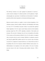
Fig. 1. Example of labelling of a chromatogram by the chromatographic response function. Blue dots denote components separated with resolutions higher than 1 from all
other peaks; red dots denote peaks that are within proximity to neighbors and are clustered together, illustrated by the red lines. (For interpretation of the references to
colour in this figure legend, the reader is referred to the web version of this article.)

real experiments, it generally becomes difficult to determine accurate values of the width of peaks (and thus the resolution between them) when peaks are close to each other. In addition, it
is often not possible to deduce how many analytes are under a
peak. With our proposed chromatographic response function we
aim to capture these effects so that it is representative for real
situations.
Fig. 1 shows an example of an evaluation by the chromatographic response function of a chromatogram of 50 analytes. 48
compounds are visible within the time constraints, denoted by
the blue and red dots. Blue dots denote compounds that are separated from all neighboring peaks by a resolution factor larger
than 1, while red dots are peaks that are connected to one or
more overlapping neighboring peaks. These connections between
pairs of peaks with resolution factors less than 1 are shown by
the red lines. Of the 48 peaks, 21 peaks are considered separated
and hence are counted as 21 connected components. The other 27

peaks are clustered together into 10 connected components and
are counted as such. Therefore this chromatogram would have a
score of 31 (21 + 10) connected components.

than an equally spaced grid. Other instrumental parameters used
for retention modeling are shown in Table 1. These instrumental parameters were chosen to reflect realistic separations that are
used in practical applications [7], and are kept fixed throughout
the experiments. In addition, we chose to use realistic theoretical
plate numbers (100 in both dimensions) that are much in line with
practical systems, and with theoretical considerations which take
into account the effects of under-sampling and injection volumes
[32].
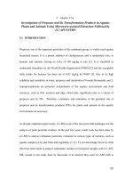
Fig. 2 shows the results of the grid search for samples of 50
compounds generated using strategy A-D (Section 3.2) and labeled
as such. Here, the number of experiments of the grid search resulting in a specific number of connected components (i.e. separated
peaks) are shown by a histogram.
Interestingly, in all samples (A-D), the grid search did not find
a solution in which all 50 analytes are separated. In fact, the maximum number of connected components (denoted by the green
vertical dashed line) were 32, 23, 38, and 35 for samples A-D respectively. While the coarse grid search was not expected to yield
the true global maximum, it did yield a benchmark for comparison with the random search and Bayesian optimization. In addition, the grid search revealed that most combinations of gradient
parameters in fact led to a low number of connected components
(compared to the maximum) and thus a relatively poor separation.
Only a limited fraction of the grid-search experiments was found
to lead to separations with a greater number of connected components. Therefore, it was deemed likely that only very small regions
of the parameter space led to good separations, potentially leading
to narrow hills and broad plateaus in the optimization landscape.
However, this is hard to visualize in 8 dimensions. For 1D-LC experiments, Huygens et al. [9] visualized that the landscape (for a
different sample than ours) in fact is non-convex and shows an increasing number of local optima with an increase in the number
of components and a decrease in column-efficiency.

4.2. Grid search
To set a benchmark for the Bayesian optimization algorithm,
a grid search was performed on 8 gradient parameters using a
grid specified in Table 3. Although this grid is relatively coarse,
it already consists out of 11,664 experiments, supporting the fact
that grid searches quickly become unfeasible as the grid becomes
increasingly fine and/or the number of parameters increases. To
save computational resources, some parameters were chosen with
a greater number of steps than others. For example, the initial time
(tinit ) was chosen to be coarser than the gradient time (tG ) as the
former generally has less impact on the quality of the separation
than the latter. In this way the grid search was more informative
6


J. Boelrijk, B. Pirok, B. Ensing et al.

Journal of Chromatography A 1659 (2021) 462628

Table 2
Overview of methods for sampling retention parameters for samples A-D.

1

lnk0
1
lnkM
1
S1
1

S2
2
lnk0
2
lnkM
2
S2
2
S2

A

B

C

U ∼ (3.27, 11.79 )
U ∼ (−2.38, −1.03 )
Eq. 27
U ∼ (−0.24, 2.51 )
U ∼ (3.27, 11.79 )
U ∼ (−2.38, −1.03 )
Eq. 27
U ∼ (−0.24, 2.51 )

U ∼ (3.27, 11.79 )
U ∼ (−2.38, −1.03 )
Eq. 27
U ∼ (−0.24, 2.51 )
1

lnk0 + U ∼ (−c1 , c2 )
1
lnkM + U ∼ (−c3 , c3 )
Eq. 27
1
S2 + U ∼ (−c1 , c1 )

ln100.0839· S1 +0.5054+r2
U ∼ (100.8 , 101.6 )
1
2.501 · log S1 − 2.0822 + r1
−2
ln100.0839 ·S1 +0.5054+r2
U ∼ (100.8 , 101.6 )
2.501log2 S1 − 2.0822 + r1

D
1

ln100.0839· S1 +0.5054+r2
U ∼ (100.8 , 101.6 )
2
2.501 · log S1 − 2.0822 + r1
ln100.0839·2S1 +0.5054+r2
2
S1 + U ∼ (−c4 , c4 )
2.501log2 S1 − 2.0822 + r1
1

Table 3

Overview of method parameters considered for optimization and their corresponding
bounds and increments used for the grid search.
Parameter

Minimum value

Maximum value

Number of steps

Increment

1

0
30
0.1
0.6
0
10
0.1
0.6

10
200
0.5
1
0.2
20
0.5

1

3
6
3
3
2
4
3
3

5
34
0.2
0.2
0.2
5
0.2
0.2

tinit
1
tG
1
1
2
2
2
2

ϕinit
ϕfinal

tinit
tG

ϕinit
ϕfinal

Fig. 2. Results of the grid search comprised out of 11,664 experiments, for samples containing 50 analytes from strategy A (top-left), B (top-right), C (bottom-left) and D (top
right). The green vertical dashed line denotes the maximum number of connected components observed in the grid-search. (For interpretation of the references to colour in
this figure legend, the reader is referred to the web version of this article.)

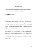
while the horizontal orange line denotes the gradient parameters
of the grid search experiment that lead to the best separation. The
black dotted vertical line denotes the upper and lower bounds that
the gradient parameters can take, which was kept similar to the
grid search. Similarly, plot I (Fig. 3) shows the number of connected components per iteration.
Interestingly, after only 42 iterations, the Bayesian optimization
algorithm was found to determine gradient parameters that improved upon the grid search maximum, by finding a method that
separated 37 connected components (compared with 35 for the

4.3. Bayesian optimization
To test the developed Bayesian optimization algorithm, we optimized 8 gradient parameters (the same as in the grid search) for a
sample of 50 compounds. The algorithm was initialized with four
randomly picked experiments, after which it was allowed to perform 100 iterations, for a total of 104 performed experiments. The
resulting runs were compared with the grid search and are shown
in Fig. 3. Plots A-H show how the gradient parameters are varied
during the Bayesian optimization run (denoted by the blue line),
7

J. Boelrijk, B. Pirok, B. Ensing et al.

Journal of Chromatography A 1659 (2021) 462628

Fig. 3. Panel containing the values of the machine parameters (A-H) and connected components (I) throughout a Bayesian optimization trial. The black dashed horizontal
lines denote the upper and lower bounds of the parameter search space. The orange line denotes the value found for the best experiment in the grid search. The vertical
grey dotted line denotes the best iteration of the Bayesian optimization algorithm.

grid search maximum). Thereafter, the algorithm continued exploration of the gradient parameters, after which it found the best
score at 74 iterations (denoted by the grey vertical dotted line).
At this iteration, the second-dimension gradient parameters are
mostly at the same value as the parameters of the grid search
maximum (indicated by the orange line). In addition, the first dimension gradient time (1 tG ) of the Bayesian optimization algorithm is quite similar to the value of the grid search maximum.
However, there is a considerable difference between the values of
the first dimension initial time 1 tinit as well as the initial 1 ϕinit and
final modifier concentration 1 ϕfinal , which led to a better separation (39 connected components) compared to the best grid search
experiment (35 connected components).
Both the best chromatogram of grid search (out of 11,664 experiments) and the Bayesian optimization run (out of 104 experiments) are shown in Fig. 4. The best experiment of the grid search
managed to elute 48 out of the 50 components within the given
time constraints (200, 2.26). Out of these 48 components, 21 peaks
were concentrated in eight clusters of peaks denoted by the red
lines in the figure. A score of 35 connected components was observed, which essentially is the number of peaks that can be distinguished from each other, similar to real experiments. The best
method of the Bayesian optimization run managed to elute all 50
components within the time constraints, with 19 peaks concentrated in 8 clusters, leading to a score of 39 connected components.
For the experienced chromatographer, it can be seen that the elongated initial time, complemented with the higher initial and final
modifier concentration, led to a compression of the first dimension, which allowed for the elution of two more peaks within the
time constraints, without creating more unresolved components.
Many clusters in the chromatogram, e.g. the clusters around 160

minutes in the grid search chromatogram, and 150 minutes in the
Bayesian optimization chromatogram, have not changed. It is likely
that these clusters, given the current simple gradient program cannot be separated, as retention parameters are simply too similar.
Increasing column efficiency, experiment duration, or complexity
of the gradient program might be able to resolve this.
4.4. Comparison of Bayesian optimization with benchmarks
Generally, in the initial iterations of the Bayesian optimization
algorithm, the algorithm operates randomly, as no clear knowledge
of how parameters influence each other is available to the model
up to that point. Therefore, in the initial phase, the algorithm is
dependent on the choice of random seed and the choice of initialization experiments, which could influence the remainder of the
optimization. Especially in scenarios such as direct experimental
optimization, where performing experiments is both timely and
costly, there is no luxury of testing multiple random seeds or many
initial experiments. For this reason, it is interesting to investigate
the worst-case performance. To investigate this, 100 trials with different random seeds were performed for each case. The algorithm
was initialized with 4 random data points and was allowed to perform 100 iterations, adding up to a total of 104 performed experiments. For a fair comparison, the random search algorithm was
also run for 100 trials with different random seeds and 104 iterations. The results of which are shown in Fig. 5.
Fig. 5 shows a comparison of the random search, grid search,
and the Bayesian optimization algorithm, for samples A-D (and
labeled as such). It can be seen that the Bayesian optimization
algorithm (shown in orange) generally outperformed the random
search (shown in blue), only in sporadic cases (less than 5%) did
8


J. Boelrijk, B. Pirok, B. Ensing et al.

Journal of Chromatography A 1659 (2021) 462628

Fig. 4. Chromatograms of the best experiment in the grid search (left) with a score of 35 connected components, and the best experiment in the Bayesian optimization trial
(right) with a score of 39 connected components.

Fig. 5. Comparison of the random search, grid search and Bayesian optimization algorithm for sample A (top-left), B (top-right), C (bottom-left) and D (bottom-right) for 100
trials. The vertical black dashed line shows the maximum observed in the grid search (out of 11,664 experiments), while the blue and orange bars denote the best score out
104 iterations for the random search and Bayesian optimization algorithm, respectively. Note that the y-axis is normalized, so that it represents the fraction of times out of
100 trials. (For interpretation of the references to colour in this figure legend, the reader is referred to the web version of this article.)

the random search find a better maximum score in 104 iterations
than the Bayesian optimization algorithm did. In addition, the random search was found to only rarely locate the same maximum as
the grid search (denoted by the vertical black dashed line), around
10% in the case of sample C, and even less for samples A (0%), B
(3%) and D (2%). It may not be surprising that a random search
over 104 iterations underperforms versus a grid search with 11,664
experiments. However, when only a small number of the gradient
parameters affect the final performance of the separation, random
search can outperform grid search [10]. Since this is not the case,
this validates the usefulness of our gradient parameters to some
extent. In addition, if the Bayesian optimization algorithm would
have similar performance as the random search, it could well be
that our Bayesian optimization approach is (i) not working as it
should be, or (ii) the problem is not challenging enough, as gradient parameters that lead to good separations can be easily found

randomly. Therefore the comparison of an algorithm with baseline
methods is paramount.
When comparing the performance of the Bayesian optimization algorithm to the maximum observed score of the grid search
(Fig. 5, denoted by the vertical black dotted line), it can be seen
that in all cases (A-D), the Bayesian optimization algorithm finds
methods that have a greater number of connected components

compared to the maximum of the grid search. This is quite remarkable, considering the difference in performed experiments for
the Bayesian optimization algorithm (104) and the grid search
(11664). However, in the 100 performed trials and 104 iterations,
the Bayesian optimization algorithm does not always find a better
score than the grid search, but is on par or better than the grid
search in 29%, 85%, 99%, and 84%, for cases A-D respectively. As we
are interested in the worst-case performance, it is of use to know
what the maximum number of iterations is before the Bayesian
9


J. Boelrijk, B. Pirok, B. Ensing et al.

Journal of Chromatography A 1659 (2021) 462628

Fig. 6. Number of iterations needed for the Bayesian optimization algorithm to reach the grid search maximum for sample A (top-left), B (top-right), C (bottom-left) and D
(bottom-right) for 100 trials with different random seeds. The grey line denotes the cumulative distribution function (CDF). The black vertical line denotes the number of
initial random observations with which the Bayesian optimization algorithm is initialized.

optimization algorithm outperforms the grid search. This is further
investigated in the next section. Note that the results for sample
A are significantly worse than the other samples, and it remains
somewhat unclear as to why this is. It could be ascribed to the
landscape, which might contain sharp narrow optima which are
bypassed easily by the Bayesian optimization algorithm and take
a considerable amount of iterations to detect. Further analysis indeed showed that the algorithm found methods with scores of 29
rather quickly (roughly 85% in less than 150 iterations), which is
shown in Figure S-4. Improving upon this score, then proved to
take considerably longer, supporting the fact that these are regions
in the gradient parameters that are difficult to pinpoint. Recognizing such behavior and stopping the optimization process or alerting the user might be useful in these cases.

mum, which is still a considerably lower number of experiments
than the grid search (11664 experiments). In addition, most trials finished quicker, as only 20% of the trials needed more than
300 iterations to reach the grid search maximum. Despite this, it
could still be argued that this is a high number of experiments for
direct experimental optimization. However, in this work, we initialize the algorithm with randomly drawn experiments. A more
sophisticated choice of initialization could provide the algorithm
with more informative initial data, which could in turn improve
the performance of the algorithm. Likewise, a more informed and
narrow range of gradient parameters, provided by expert knowledge, could improve things even further.

4.5. Iterations needed to obtain grid search maximum

We have applied Bayesian optimization and demonstrated its
capability of maximizing a novel chromatographic response function to optimize eight gradient parameters in comprehensive twodimensional liquid chromatography (LC×LC). The algorithm was
tested for worst-case performance on four different samples of 50
compounds by repeating the optimization loop for 100 trials with
different random seeds. The algorithm was benchmarked against a
grid search (consisting out of 11,664 experiments) and a random
search policy. Given an optimization budget of 100 iterations, the
Bayesian optimization algorithm generally outperformed the random search and often improved upon the grid search. The Bayesian
optimization algorithm was on par, for all trials, with the grid
search after 700 iterations for case A, and less than 250 iterations
for cases B-D, which was a significant speed-up compared to the
grid search (a factor 10 to 100). In addition, it generally takes much
shorter than that, as 80% or more of the trials converged at less
than 100 iterations for samples B-D. This could likely be further
improved by a more informed choice of the initialization experiments (which were randomly picked in this study), which could
be provided by the analyst’s experience or smarter procedures.

5. Conclusion

We now turn to how many iterations it would take for the
Bayesian optimization algorithm to reach the same maximum as
that was found in the grid search for each respective case. This was
done by running the Bayesian optimization algorithm 100 times
with different random seeds until the grid search maximum of the
respective cases (A-D) was observed. The results of this analysis
are shown in Fig. 6, where the blue bars indicate how often a specific trial found the grid search maximum at a specific iteration.
The dark-grey line then shows the cumulative distribution function (CDF) which describes what percentage of trials converged as
a function of iterations.
From Fig. 6 it can be seen that for samples B (∼85%), C (∼95%),
and D (∼82%) most of the trials converged after performing 100
iterations or less, this is much in line with the results of the previous section. The remaining trials then took anywhere between
100 and 204 (B), 230 (C), or 231 (D) iterations. Sample A again
proved to be intrinsically harder than samples B, C, and D, yet after 700 iterations, all the 100 trials found the grid search maxi10


J. Boelrijk, B. Pirok, B. Ensing et al.

Journal of Chromatography A 1659 (2021) 462628

We have shown that Bayesian optimization is a viable method
for optimization in retention modeling with many method parameters, and therefore also for direct experimental optimization of
simple to moderate separation problems. Yet, this study was conducted under a simplified chromatographic reality (Gaussian peaks
and equal concentration of analytes, generated compounds). Evidently, a follow-up study will have to focus on the effect of these
non-idealities, using the current results as a benchmark to measure
these effects against. In addition, to apply this approach to direct
experimental optimization, its success is largely dependent on data
processing algorithms such as peak detection and peak tracking algorithms to obtain an accurate and consistent assessment of the

quality of separations. Nevertheless, it is evident that Bayesian optimization could play a vital role in automated direct experimental
optimization.

[6] J.W. Dolan, D.C. Lommen, L.R. Snyder, Drylab® computer simulation for highperformance liquid chromatographic method development. II. Gradient Elution,
1989, 10.1016/S0021-9673(01)89134-2
[7] B.W. Pirok, S. Pous-Torres, C. Ortiz-Bolsico, G. Vivó-Truyols, P.J. Schoenmakers, Program for the interpretive optimization of two-dimensional resolution,
J. Chromatogr. A 1450 (2016) 29–37, doi:10.1016/j.chroma.2016.04.061.
[8] W. Hao, B. Li, Y. Deng, Q. Chen, L. Liu, Q. Shen, Computer aided optimization
of multilinear gradient elution in liquid chromatography, J. Chromatogr. A 1635
(2021) 461754, doi:10.1016/j.chroma.2020.461754.
[9] B. Huygens, K. Efthymiadis, A. Nowé, G. Desmet, Application of evolutionary
algorithms to optimise one- and two-dimensional gradient chromatographic
separations, J. Chromatogr. A 1628 (2020) 461435, doi:10.1016/j.chroma.2020.
461435.
[10] J. Bergstra, R. Bardenet, Y. Bengio, B. Kégl, Algorithms for hyper-parameter optimization, Adv Neural Inf Process Syst 24 (2011).
[11] D. Lizotte, T. Wang, M. Bowling, D. Schuurmans, Automatic gait optimization
with Gaussian process regression, IJCAI International Joint Conference on Artificial Intelligence (2007) 944–949.
[12] R. Marchant, F. Ramos, Bayesian optimisation for intelligent environmental
monitoring, IEEE International Conference on Intelligent Robots and Systems
(2012) 2242–2249, doi:10.1109/IROS.2012.6385653.
[13] J. Azimi, A. Jalali, X. Fern, Hybrid batch Bayesian optimization, Proceedings of
the 29th International Conference on Machine Learning, ICML 2012 2 (2012)
1215–1222.
[14] S. Daulton, M. Balandat, E. Bakshy, Differentiable expected hypervolume improvement for parallel multi-objective Bayesian optimization, arXiv (2020).
[15] A. Kensert, G. Collaerts, K. Efthymiadis, G. Desmet, D. Cabooter, Deep Qlearning for the selection of optimal isocratic scouting runs in liquid chromatography, J. Chromatogr. A 1638 (2021) 461900, doi:10.1016/j.chroma.2021.
461900.
[16] P. Nikitas, A. Pappa-Louisi, Retention models for isocratic and gradient elution
in reversed-phase liquid chromatography, J. Chromatogr. A 1216 (10) (2009)
1737–1755, doi:10.1016/j.chroma.2008.09.051.
[17] U.D. Neue, H.J. Kuss, Improved reversed-phase gradient retention modeling, J.

Chromatogr. A 1217 (24) (2010) 3794–3803, doi:10.1016/j.chroma.2010.04.023.
[18] U.D. Neue, D.H. Marchand, L.R. Snyder, Peak compression in reversed-phase
gradient elution, J. Chromatogr. A 1111 (1) (2006) 32–39, doi:10.1016/j.chroma.
2006.01.104.
[19] H. Poppe, J. Paanakker, M. Bronckhorst, Peak width in solvent-programmed
chromatography : I. general description of peak broadening in solventprogrammed elution, J. Chromatogr. A 204 (C) (1981) 77–84, doi:10.1016/
S0 021-9673(0 0)81641-6.
[20] J. Snoek, H. Larochelle, R.P. Adams, Practical bayesian optimization of machine
learning algorithms, Adv Neural Inf Process Syst 4 (2012) 2951–2959.
[21] C. Oh, E. Gavves, M. Welling, BOCK : Bayesian optimization with cylindrical kernels, Proceedings of Machine Learning Research (2018) 3868–3877.
[22] C.E. Rasmussen, Gaussian Processes in Machine Learning, Springer Verlag,
2004, pp. 63–71, doi:10.1007/978- 3- 540- 28650- 9_4.
[23] B. Shahriari, K. Swersky, Z. Wang, R.P. Adams, N. De Freitas, Taking the human
out of the loop: a review of Bayesian optimization, Proc. IEEE 104 (1) (2016)
148–175, doi:10.1109/JPROC.2015.2494218.
[24] A.D. Bull, Convergence rates of efficient global optimization algorithms, Journal
of Machine Learning Research 12 (2011) 2879–2904.
[25] J. Bergstra, Y. Bengio, Random search for hyper-parameter optimization, Journal
of Machine Learning Research 13 (2012) 281–305.
[26] M. Balandat, B. Karrer, D.R. Jiang, S. Daulton, B. Letham, A.G. Wilson, E. Bakshy, BoTorch: a framework for efficient monte-carlo Bayesian optimization, Adv
Neural Inf Process Syst 33 (2020).
[27] J.R. Gardner, G. Pleiss, D. Bindel, K.Q. Weinberger, A.G. Wilson, Gpytorch: blackbox matrix-matrix Gaussian process inference with GPU acceleration, in: Advances in Neural Information Processing Systems, volume 2018-Decem, 2018,
pp. 7576–7586.
[28] B.W. Pirok, S.R. Molenaar, R.E. van Outersterp, P.J. Schoenmakers, Applicability of retention modelling in hydrophilic-interaction liquid chromatography for
algorithmic optimization programs with gradient-scanning techniques, J. Chromatogr. A 1530 (2017) 104–111, doi:10.1016/j.chroma.2017.11.017.
[29] J.T. Matos, R.M. Duarte, A.C. Duarte, Trends in data processing of comprehensive two-dimensional chromatography: state of the art, Journal of Chromatography B: Analytical Technologies in the Biomedical and Life Sciences 910
(2012) 31–45, doi:10.1016/j.jchromb.2012.06.039.
[30] J.T. Matos, R.M. Duarte, A.C. Duarte, Chromatographic response functions in 1D
and 2D chromatography as tools for assessing chemical complexity, Trends in
Analytical Chemistry 45 (2013) 14–23, doi:10.1016/j.trac.2012.12.013.

[31] M.R. Schure, Quantification of resolution for two-dimensional separations, J.
Microcolumn Sep. 9 (3) (1997) 169–176, doi:10.1002/(sici)1520-667x(1997)9:
3 169::aid- mcs5 3.0.co;2- 23.
[32] G. Vivó-Truyols, S. Van Der Wal, P.J. Schoenmakers, Comprehensive study
on the optimization of online two-dimensional liquid chromatographic systems considering losses in theoretical peak capacity in first- and seconddimensions: apareto-optimality approach, Anal. Chem. 82 (20) (2010) 8525–
8536, doi:10.1021/ac101420f.

Declaration of Competing Interest
The authors declare that they have no known competing financial interests or personal relationships that could have appeared to
influence the work reported in this paper.
CRediT authorship contribution statement
Jim Boelrijk: Conceptualization, Investigation, Data curation,
Formal analysis, Methodology, Writing – original draft. Bob Pirok:
Methodology, Supervision, Writing – review & editing. Bernd Ensing: Supervision, Writing – review & editing, Funding acquisition.
Patrick Forré: Methodology, Supervision, Writing – review & editing.
Acknowledgements
Special thanks to Stef Molenaar, Tijmen Bos, and ChangYong Oh
for helpful discussions and insights. This work was performed in
the context of the Chemometrics and Advanced Separations Team
(CAST) within the Centre Analytical Sciences Amsterdam (CASA).
The valuable contributions of the CAST members are gratefully acknowledged.
Supplementary material
Supplementary material associated with this article can be
found, in the online version, at doi:10.1016/j.chroma.2021.462628.
References
[1] A. D’Attoma, C. Grivel, S. Heinisch, On-line comprehensive two-dimensional
separations of charged compounds using reversed-phase high performance liquid chromatography and hydrophilic interaction chromatography. part i: orthogonality and practical peak capacity considerations, J. Chromatogr. A 1262
(2012) 148–159, doi:10.1016/j.chroma.2012.09.028.
[2] R.J. Vonk, A.F. Gargano, E. Davydova, H.L. Dekker, S. Eeltink, L.J. De Koning, P.J. Schoenmakers, Comprehensive two-dimensional liquid chromatography with stationary-phase-assisted modulation coupled to high-resolution
mass spectrometry applied to proteome analysis of saccharomyces cerevisiae,

Anal. Chem. 87 (10) (2015) 5387–5394, doi:10.1021/acs.analchem.5b00708.
[3] P. Dugo, N. Fawzy, F. Cichello, F. Cacciola, P. Donato, L. Mondello, Stop-flow
comprehensive two-dimensional liquid chromatography combined with mass
spectrometric detection for phospholipid analysis, J. Chromatogr. A 1278 (2013)
46–53, doi:10.1016/j.chroma.2012.12.042.
[4] M.J. den Uijl, P.J. Schoenmakers, G.K. Schulte, D.R. Stoll, M.R. van Bommel,
B.W. Pirok, Measuring and using scanning-gradient data for use in method
optimization for liquid chromatography, J. Chromatogr. A 1636 (2021) 461780,
doi:10.1016/j.chroma.2020.461780.
[5] B.W. Pirok, S.R. Molenaar, L.S. Roca, P.J. Schoenmakers, Peak-Tracking algorithm for use in automated interpretive method-development tools in liquid chromatography, Anal. Chem. 90 (23) (2018) 14011–14019, doi:10.1021/acs.
analchem.8b03929.

11