Báo cáo khoa học: "Optimal Head-Driven Parsing Complexity for Linear Context-Free Rewriting Systems" docx

Proceedings of the 49th Annual Meeting of the Association for Computational Linguistics, pages 450–459,
Portland, Oregon, June 19-24, 2011.
c
2011 Association for Computational Linguistics
Optimal Head-Driven Parsing Complexity
for Linear Context-Free Rewriting Systems
Pierluigi Crescenzi
Dip. di Sistemi e Informatica
Universit
`
a di Firenze
Daniel Gildea
Computer Science Dept.
University of Rochester
Andrea Marino
Dip. di Sistemi e Informatica
Universit
`
a di Firenze
Gianluca Rossi
Dip. di Matematica
Universit
`
a di Roma Tor Vergata
Giorgio Satta
Dip. di Ingegneria dell’Informazione
Universit
`
a di Padova
Abstract
Westudy the problem of finding the best head-

driven parsing strategy for Linear Context-
Free Rewriting System productions. A head-
driven strategy must begin with a specified
righthand-side nonterminal (the head) and add
the remaining nonterminals one at a time in
any order. We show that it is NP-hard to find
the best head-driven strategy in terms of either
the time or space complexity of parsing.
1 Introduction
Linear Context-Free Rewriting Systems (LCFRSs)
(Vijay-Shankar et al., 1987) constitute a very general
grammatical formalism which subsumes context-
free grammars (CFGs) and tree adjoining grammars
(TAGs), as well as the synchronous context-free
grammars (SCFGs) and synchronous tree adjoin-
ing grammars (STAGs) used as models in machine
translation.
1
LCFRSs retain the fundamental prop-
erty of CFGs that grammar nonterminals rewrite
independently, but allow nonterminals to generate
discontinuous phrases, that is, to generate more
than one span in the string being produced. This
important feature has been recently exploited by
Maier and Søgaard (2008) and Kallmeyer and Maier
(2010) for modeling phrase structure treebanks with
discontinuous constituents, and by Kuhlmann and
Satta (2009) for modeling non-projective depen-
dency treebanks.
The rules of a LCFRS can be analyzed in terms

of the properties of rank and fan-out. Rank is the
1
To be more precise, SCFGs and STAGs generate languages
composed by pair of strings, while LCFRSs generate string lan-
guages. We can abstract away from this difference by assuming
concatenation of components in a string pair.
number of nonterminals on the right-hand side (rhs)
of a rule, while fan-out is the number of spans of
the string generated by the nonterminal in the left-
hand side (lhs) of the rule. CFGs are equivalent to
LCFRSs with fan-out one, while TAGs are one type
of LCFRSs with fan-out two. Rambow and Satta
(1999) show that rank and fan-out induce an infi-
nite, two-dimensional hierarchy in terms of gener-
ative power; while CFGs can always be reduced to
rank two (Chomsky Normal Form), this is not the
case for LCFRSs with any fan-out greater than one.
General algorithms for parsing LCFRSs build a
dynamic programming chart of recognized nonter-
minals bottom-up, in a manner analogous to the
CKY algorithm for CFGs (Hopcroft and Ullman,
1979), but with time and space complexity that are
dependent on the rank and fan-out of the gram-
mar rules. Whenever it is possible, binarization of
LCFRS rules, or reduction of rank to two, is there-
fore important for parsing, as it reduces the time
complexity needed for dynamic programming. This
has lead to a number of binarization algorithms for
LCFRSs, as well as factorization algorithms that
factor rules into new rules with smaller rank, with-

out necessarily reducing rank all the way to two.
Kuhlmann and Satta (2009) present an algorithm
for binarizing certain LCFRS rules without increas-
ing their fan-out, and Sagot and Satta (2010) show
how to reduce rank to the lowest value possible for
LCFRS rules of fan-out two, again without increas-
ing fan-out. G
´
omez-Rodr
´
ıguez et al. (2010) show
how to factorize well-nested LCFRS rules of arbi-
trary fan-out for efficient parsing.
In general there may be a trade-off required
between rank and fan-out, and a few recent pa-
pers have investigated this trade-off taking gen-
450
eral LCFRS rules as input. G
´
omez-Rodr
´
ıguez et
al. (2009) present an algorithm for binarization of
LCFRSs while keeping fan-out as small as possi-
ble. The algorithm is exponential in the resulting
fan-out, and G
´
omez-Rodr
´
ıguez et al. (2009) mention

as an important open question whether polynomial-
time algorithms to minimize fan-out are possible.
Gildea (2010) presents a related method for bina-
rizing rules while keeping the time complexity of
parsing as small as possible. Binarization turns out
to be possible with no penalty in time complexity,
but, again, the factorization algorithm is exponen-
tial in the resulting time complexity. Gildea (2011)
shows that a polynomial time algorithm for factor-
izing LCFRSs in order to minimize time complexity
would imply an improved approximation algorithm
for the well-studied graph-theoretic property known
as treewidth. However, whether the problem of fac-
torizing LCFRSs in order to minimize time com-
plexity is NP-hard is still an open question in the
above works.
Similar questions have arisen in the context of
machine translation, as the SCFGs used to model
translation are also instances of LCFRSs, as already
mentioned. For SCFG, Satta and Peserico (2005)
showed that the exponent in the time complexity
of parsing algorithms must grow at least as fast as
the square root of the rule rank, and Gildea and
ˇ
Stefankovi
ˇ
c (2007) tightened this bound to be lin-
ear in the rank. However, neither paper provides an
algorithm for finding the best parsing strategy, and
Huang et al. (2009) mention that whether finding the

optimal parsing strategy for an SCFG rule is NP-
hard is an important problem for future work.
In this paper, we investigate the problem of rule
binarization for LCFRSs in the context of head-
driven parsing strategies. Head-driven strategies be-
gin with one rhs symbol, and add one nontermi-
nal at a time. This rules out any factorization in
which two subsets of nonterminals of size greater
than one are combined in a single step. Head-driven
strategies allow for the techniques of lexicalization
and Markovization that are widely used in (projec-
tive) statistical parsing (Collins, 1997). The statis-
tical LCFRS parser of Kallmeyer and Maier (2010)
binarizes rules head-outward, and therefore adopts
what we refer to as a head-driven strategy. How-
ever, the binarization used by Kallmeyer and Maier
(2010) simply proceeds left to right through the rule,
without considering the impact of the parsing strat-
egy on either time or space complexity. We examine
the question of whether we can efficiently find the
strategy that minimizes either the time complexity
or the space complexity of parsing. While a naive
algorithm can evaluate all r! head-driven strategies
in time O(n · r!), where r is the rule’s rank and n
is the total length of the rule’s description, we wish
to determine whether a polynomial-time algorithm
is possible.
Since parsing problems can be cast in terms of
logic programming (Shieber et al., 1995), we note
that our problem can be thought of as a type of

query optimization for logic programming. Query
optimization for logic programming is NP-complete
since query optimization for even simple conjunc-
tive database queries is NP-complete (Chandra and
Merlin, 1977). However, the fact that variables in
queries arising from LCFRS rules correspond to the
endpoints of spans in the string to be parsed means
that these queries have certain structural properties
(Gildea, 2011). We wish to determine whether the
structure of LCFRS rules makes efficient factoriza-
tion algorithms possible.
In the following, we show both the the time- and
space-complexity problems to be NP-hard for head-
driven strategies. We provide what is to our knowl-
edge the first NP-hardness result for a grammar fac-
torization problem, which we hope will aid in under-
standing parsing algorithms in general.
2 LCFRSs and parsing complexity
In this section we briefly introduce LCFRSs and de-
fine the problem of optimizing head-driven parsing
complexity for these formalisms. For a positive in-
teger n, we write [n] to denote the set {1, . . . , n}.
As already mentioned in the introduction,
LCFRSs generate tuples of strings over some finite
alphabet. This is done by associating each produc-
tion p of a grammar with a function g that takes as
input the tuples generated by the nonterminals in p’s
rhs, and rearranges their string components into a
new tuple, possibly adding some alphabet symbols.
Let V be some finite alphabet. We write V

∗
for
the set of all (finite) strings over V . For natural num-
bers r ≥ 0 and f, f
1
, . . . , f
r
≥ 1, consider a func-
451
tion g : (V
∗
)
f
1
× · · · × (V
∗
)
f
r
→ (V
∗
)
f
defined by
an equation of the form
g(x
1,1
, . . . , x
1,f
1

, . . . , x
r,1
, . . . , x
r,f
r
) = α .
Here the x
i,j
’s denote variables over strings in V
∗
,
and α = α
1
, . . . , α
f
 is an f-tuple of strings over
g’s argument variables and symbols in V . We say
that g is linear, non-erasing if α contains exactly
one occurrence of each argument variable. We call r
and f the rank and the fan-out of g, respectively,
and write r(g) and f(g) to denote these quantities.
Example 1 g
1
(x
1,1
, x
1,2
) = x
1,1
x

1,2
 takes as
input a tuple with two strings and returns a tuple
with a single string, obtained by concatenating the
components in the input tuple. g
2
(x
1,1
, x
1,2
) =
ax
1,1
b, cx
1,2
d takes as input a tuple with two
strings and wraps around these strings with sym-
bols a, b, c, d ∈ V . Both functions are linear, non-
erasing, and we have r(g
1
) = r(g
2
) = 1, f(g
1
) = 1
and f(g
2
) = 2.
✷
A linear context-free rewriting system is a tuple

G = (V
N
, V
T
, P, S), where V
N
and V
T
are finite,
disjoint alphabets of nonterminal and terminal sym-
bols, respectively. Each A ∈ V
N
is associated with
a value f (A), called its fan-out. The nonterminal S
is the start symbol, with f (S) = 1. Finally, P is a
set of productions of the form
p : A → g(A
1
, A
2
, . . . , A
r(g)
) , (1)
where A, A
1
, . . . , A
r(g)
∈ V
N
, and g : (V

∗
T
)
f(A
1
)
× · · · × (V
∗
T
)
f(A
r(g)
)
→ (V
∗
T
)
f(A)
is a linear, non-
erasing function.
Production (1) can be used to transform the
r(g) string tuples generated by the nonterminals
A
1
, . . . , A
r(g)
into a tuple of f(A) strings gener-
ated by A. The values r(g) and f(g) are called the
rank and fan-out of p, respectively, written r(p) and
f(p). Given that f(S) = 1, S generates a set of

strings, defining the language L(G).
Example 2 Let g
1
and g
2
be as in Example 1, and
let g
3
() = ε, ε. Consider the LCFRS G defined by
the productions p
1
: S → g
1
(A), p
2
: A → g
2
(A)
and p
3
: A → g
3
(). We have f (S) = 1, f(A) =
f(G) = 2, r(p
3
) = 0 and r(p
1
) = r(p
2
) = r(G) =

1. We have L(G) = {a
n
b
n
c
n
d
n
| n ≥ 1}. For in-
stance, the string a
3
b
3
c
3
d
3
is generated by means
fan-out
strategy
4 ((A
1
⊕ A
4
) ⊕ A
3
)
∗
⊕ A
2

3
(A
1
⊕ A
4
)
∗
⊕ (A
2
⊕ A
3
)
3
((A
1
⊕ A
2
)
∗
⊕ A
4
) ⊕ A
3
2
((A
∗
2
⊕ A
3
) ⊕ A

4
) ⊕ A
1
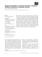
Figure 1: Some parsing strategies for production p in Ex-
ample 3, and the associated maximum value for fan-out.
Symbol ⊕ denotes the merging operation, and superscript
∗ marks the first step in the strategy in which the highest
fan-out is realized.
of the following bottom-up process. First, the tuple
ε, ε is generated by A through p
3
. We then iterate
three times the application of p
2
to ε, ε, resulting
in the tuple a
3
b
3
, c
3
d
3
. Finally, the tuple (string)
a
3
b
3
c
3

d
3
 is generated by S through application of
p
1
.
✷
Existing parsing algorithms for LCFRSs exploit
dynamic programming. These algorithms compute
partial parses of the input string w, represented by
means of specialized data structures called items.
Each item indexes the boundaries of the segments
of w that are spanned by the partial parse. In the
special case of parsing based on CFGs, an item con-
sists of two indices, while for TAGs four indices are
required.
In the general case of LCFRSs, parsing of a pro-
duction p as in (1) can be carried out in r (g) − 1
steps, collecting already available parses for nonter-
minals A
1
, . . . , A
r(g)
one at a time, and ‘merging’
these into intermediate partial parses. We refer to the
order in which nonterminals are merged as a pars-
ing strategy, or, equivalently, a factorization of the
original grammar rule. Any parsing strategy results
in a complete parse of p, spanning f(p) = f(A)
segments of w and represented by some item with

2f(A) indices. However, intermediate items ob-
tained in the process might span more than f(A)
segments. We illustrate this through an example.
Example 3 Consider a linear non-erasing function
g(x
1,1
, x
1,2
, x
2,1
, x
2,2
, x
3,1
, x
3,2
, x
4,1
, x
4,2
)
= x
1,1
x
2,1
x
3,1
x
4,1
, x

3,2
x
2,2
x
4,2
x
1,2
, and a pro-
duction p : A → g(A
1
, A
2
, A
3
, A
4
), where all the
nonterminals involved have fan-out 2. We could
parse p starting from A
1
, and then merging with A
4
,
452
v
1
v
2
v
3

v
4
e
1
e
3
e
2
e
4
Figure 2: Example input graph for our construction of an
LCFRS production.
A
3
, and A
2
. In this case, after we have collected the
first three nonterminals, we have obtained a partial
parse having fan-out 4, that is, an item spanning 4
segments of the input string. Alternatively, we could
first merge A
1
and A
4
, then merge A
2
and A
3
, and
finally merge the two obtained partial parses. This

strategy is slightly better, resulting in a maximum
fan-out of 3. Other possible strategies can be ex-
plored, displayed in Figure 1. It turns out that the
best parsing strategy leads to fan-out 2.
✷
The maximum fan-out f realized by a parsing
strategy determines the space complexity of the
parsing algorithm. For an input string w, items will
require (in the worst-case) 2f indices, each taking
O(|w|) possible values. This results in space com-
plexity of O(|w|
2f
). In the special cases of parsing
based on CFGs and TAGs, this provides the well-
known space complexity of O(|w|
2
) and O(|w|
4
),
respectively.
It can also be shown that, if a partial parse hav-
ing fan-out f is obtained by means of the combi-
nation of two partial parses with fan-out f
1
and f
2
,
respectively, the resulting time complexity will be
O(|w|
f+f

1
+f
2
) (Seki et al., 1991; Gildea, 2010). As
an example, in the case of parsing based on CFGs,
nonterminals as well as partial parses all have fan-
out one, resulting in the standard time complexity of
O(|w|
3
) of dynamic programming methods. When
parsing with TAGs, we have to manipulate objects
with fan-out two (in the worst case), resulting in time
complexity of O(|w|
6
).
We investigate here the case of general LCFRS
productions, whose internal structure is consider-
ably more complex than the context-free or the tree
adjoining case. Optimizing the parsing complexity
for a production means finding a parsing strategy
that results in minimum space or time complexity.
We now turn the above optimization problems
into decision problems. In the MIN SPACE STRAT-
EGY problem one takes as input an LCFRS produc-
tion p and an integer k, and must decide whether
there exists a parsing strategy for p with maximum
fan-out not larger than k. In the MIN TIME STRAT-
EGY problem one is given p and k as above and must
decide whether there exists a parsing strategy for
p such that, in any of its steps merging two partial

parses with fan-out f
1
and f
2
and resulting in a par-
tial parse with fan-out f, the relation f +f
1
+f
2
≤ k
holds.
In this paper we investigate the above problems in
the context of a specific family of linguistically mo-
tivated parsing strategies for LCFRSs, called head-
driven. In a head-driven strategy, one always starts
parsing a production p from a fixed nonterminal in
its rhs, called the head of p, and merges the remain-
ing nonterminals one at a time with the partial parse
containing the head. Thus, under these strategies,
the construction of partial parses that do not include
the head is forbidden, and each parsing step involves
at most one partial parse. In Figure 1, all of the dis-
played strategies but the one in the second line are
head-driven (for different choices of the head).
3 NP-completeness results
For an LCFRS production p, let H be its head non-
terminal, and let A
1
, . . . , A
n

be all the non-head
nonterminals in p’s rhs, with n + 1 = r(p). A head-
driven parsing strategy can be represented as a per-
mutation π over the set [n], prescribing that the non-
head nonterminals in p’s rhs should be merged with
H in the order A
π(1)
, A
π(2)
, . . . , A
π(n)
. Note that
there are n! possible head-driven parsing strategies.
To show that MIN SPACE STRATEGY is NP-
hard under head-driven parsing strategies, we reduce
from the MIN CUT LINEAR ARRANGEMENT prob-
lem, which is a decision problem over (undirected)
graphs. Given a graph M = (V, E) with set of ver-
tices V and set of edges E, a linear arrangement
of M is a bijective function h from V to [n], where
|V | = n. The cutwidth of M at gap i ∈ [n − 1] and
with respect to a linear arrangement h is the number
of edges crossing the gap between the i-th vertex and
its successor:
cw(M, h, i) = |{(u, v) ∈ E | h(u) ≤ i < h(v)}| .
453
p : A → g(H, A
1
, A
2

, A
3
, A
4
)
g(x
H,e
1
, x
H,e
2
, x
H,e
3
, x
H,e
4
, x
A
1
,e
1
,l
, x
A
1
,e
1
,r
, x

A
1
,e
3
,l
, x
A
1
,e
3
,r
, x
A
2
,e
1
,l
, x
A
2
,e
1
,r
, x
A
2
,e
2
,l
, x

A
2
,e
2
,r
,
x
A
3
,e
2
,l
, x
A
3
,e
2
,r
, x
A
3
,e
3
,l
, x
A
3
,e
3
,r

, x
A
3
,e
4
,l
, x
A
3
,e
4
,r
, x
A
4
,e
4
,l
, x
A
4
,e
4
,r
) =
 x
A
1
,e
1

,l
x
A
2
,e
1
,l
x
H,e
1
x
A
1
,e
1
,r
x
A
2
,e
1
,r
, x
A
2
,e
2
,l
x
A

3
,e
2
,l
x
H,e
2
x
A
2
,e
2
,r
x
A
3
,e
2
,r
,
x
A
1
,e
3
,l
x
A
3
,e

3
,l
x
H,e
3
x
A
1
,e
3
,r
x
A
3
,e
3
,r
, x
A
3
,e
4
,l
x
A
4
,e
4
,l
x

H,e
4
x
A
3
,e
4
,r
x
A
4
,e
4
,r

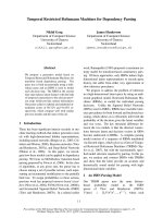
Figure 3: The construction used to prove Theorem 1 builds the LCFRS production p shown, when given as input the
graph of Figure 2.
The cutwidth of M is then defined as
cw(M) = min
h
max
i∈[n−1]
cw(M, h, i) .
In the MIN CUT LINEAR ARRANGEMENT problem,
one is given as input a graph M and an integer k, and
must decide whether cw(M) ≤ k . This problem has
been shown to be NP-complete (Gavril, 1977).
Theorem 1 The MIN SPACE STRATEGY problem
restricted to head-driven parsing strategies is NP-
complete.

PROOF We start with the NP-hardness part. Let
M = (V, E) and k be an input instance for
MIN CUT LINEAR ARRANGEMENT, and let V =
{v
1
, . . . , v
n
} and E = {e
1
, . . . , e
q
}. We assume
there are no self loops in M , since these loops do not
affect the value of the cutwidth and can therefore be
removed. We construct an LCFRS production p and
an integer k
′
as follows.
Production p has a head nonterminal H and a non-
head nonterminal A
i
for each vertex v
i
∈ V . We let
H generate tuples with a string component for each
edge e
i
∈ E. Thus, we have f (H) = q. Accord-
ingly, we use variables x
H,e

i
, for each e
i
∈ E, to
denote the string components in tuples generated by
H.
For each v
i
∈ V , let E(v
i
) ⊆ E be the set of
edges impinging on v
i
; thus |E(v
i
)| is the degree
of v
i
. We let A
i
generate a tuple with two string
components for each e
j
∈ E(v
i
). Thus, we have
f(A
i
) = 2 · |E(v
i

)|. Accordingly, we use variables
x
A
i
,e
j
,l
and x
A
i
,e
j
,r
, for each e
j
∈ E(v
i
), to de-
note the string components in tuples generated by
A
i
(here subscripts l and r indicate left and right
positions, respectively; see below).
We set r(p) = n + 1 and f(p) = q, and
define p by A → g(H, A
1
, A
2
, . . . , A
n

), with
g(t
H
, t
A
1
, . . . , t
A
n
) = α
1
, . . . , α
q
. Here t
H
is the
tuple of variables for H and each t
A
i
, i ∈ [n ], is the
tuple of variables for A
i
. Each string α
i
, i ∈ [q], is
specified as follows. Let v
s
and v
t
be the endpoints

of e
i
, with v
s
, v
t
∈ V and s < t. We define
α
i
= x
A
s
,e
i
,l
x
A
t
,e
i
,l
x
H,e
i
x
A
s
,e
i
,r

x
A
t
,e
i
,r
.
Observe that whenever edge e
i
impinges on vertex
v
j
, then the left and right strings generated by A
j
and associated with e
i
wrap around the string gen-
erated by H and associated with the same edge. Fi-
nally, we set k
′
= q + k.
Example 4 Given the input graph of Figure 2, our
reduction constructs the LCFRS production shown
in Figure 3. Figure 4 gives a visualization of how the
spans in this production fit together. For each edge
in the graph of Figure 2, we have a group of five
spans in the production: one for the head nontermi-
nal, and two spans for each of the two nonterminals
corresponding to the edge’s endpoints.
✷

Assume now some head-driven parsing strategy
π for p. For each i ∈ [n], we define D
π
i
to be the
partial parse obtained after step i in π, consisting
of the merge of nonterminals H, A
π(1)
, . . . , A
π(i)
.
Consider some edge e
j
= (v
s
, v
t
). We observe that
for any D
π
i
that includes or excludes both nontermi-
nals A
s
and A
t
, the α
j
component in the definition
of p is associated with a single string, and therefore

contributes with a single unit to the fan-out of the
partial parse. On the other hand, if D
π
i
includes only
one nonterminal between A
s
and A
t
, the α
j
compo-
nent is associated with two strings and contributes
with two units to the fan-out of the partial parse.
We can associate with π a linear arrangement h
π
of M by letting h
π
(v
π(i)
) = i, for each v
i
∈ V .
From the above observation on the fan-out of D
π
i
,
454
x
A

1
,e
1
,l
x
A
2
,e
1
,l
x
H,e
1
x
A
1
,e
1
,r
x
A
2
,e
1
,r
x
A
2
,e
2

,l
x
A
3
,e
2
,l
x
H,e
2
x
A
2
,e
2
,r
x
A
3
,e
2
,r
x
A
1
,e
3
,l
x
A

3
,e
3
,l
x
H,e
3
x
A
1
,e
3
,r
x
A
3
,e
3
,r
x
A
3
,e
4
,l
x
A
4
,e
4

,l
x
H,e
4
x
A
3
,e
4
,r
x
A
4
,e
4
,r
H
A
1
A
2
A
3
A
4
Figure 4: A visualization of how the spans for each nonterminal fit together in the left-to-right order defined by the
production of Figure 3.
we have the following relation, for every i ∈ [n−1]:
f(D
π

i
) = q + cw(M, h
π
, i) .
We can then conclude that M, k is a positive instance
of MIN CUT LINEAR ARRANGEMENT if and only
if p, k
′
is a positive instance of MIN SPACE STRAT-
EGY. This proves that MIN SPACE STRATEGY is
NP-hard.
To show that MIN SPACE STRATEGY is in NP,
consider a nondeterministic algorithm that, given an
LCFRS production p and an integer k, guesses a
parsing strategy π for p, and tests whether f(D
π
i
) ≤
k for each i ∈ [n]. The algorithm accepts or rejects
accordingly. Such an algorithm can clearly be im-
plemented to run in polynomial time.

We now turn to the MIN TIME STRATEGY prob-
lem, restricted to head-driven parsing strategies. Re-
call that we are now concerned with the quantity
f
1
+ f
2
+ f , where f

1
is the fan-out of some partial
parse D, f
2
is the fan-out of a nonterminal A, and f
is the fan out of the partial parse resulting from the
merge of the two previous analyses.
We need to introduce the MODIFIED CUTWIDTH
problem, which is a variant of the MIN CUT LIN-
EAR ARRANGEMENT problem. Let M = (V, E) be
some graph with |V | = n, and let h be a linear ar-
rangement for M. The modified cutwidth of M at
position i ∈ [n] and with respect to h is the number
of edges crossing over the i-th vertex:
mcw(M, h, i) = |{(u, v) ∈ E | h(u) < i < h(v)}| .
The modified cutwidth of M is defined as
mcw(M) = min
h
max
i∈[n]
mcw(M, h, i) .
In the MODIFIED CUTWIDTH problem one is given
as input a graph M and an integer k, and must
decide whether mcw(M ) ≤ k. The MODIFIED
CUTWIDTH problem has been shown to be NP-
complete by Lengauer (1981). We strengthen this
result below; recall that a cubic graph is a graph
without self loops where each vertex has degree
three.
Lemma 1 The MODIFIED CUTWIDTH problem re-

stricted to cubic graphs is NP-complete.
PROOF The MODIFIED CUTWIDTH problem has
been shown to be NP-complete when restricted to
graphs of maximum degree three by Makedon et al.
(1985), reducing from a graph problem known as
bisection width (see also Monien and Sudborough
(1988)). Specifically, the authors construct a graph
G
′
of maximum degree three and an integer k
′
from
an input graph G = (V, E) with an even number n
of vertices and an integer k, such that mcw(G
′
) ≤ k
′
if and only if the bisection width bw(G) of G is not
greater than k, where
bw(G) = min
A,B⊆V
|{(u, v) ∈ E | u ∈ A ∧ v ∈ B}|
with A ∩ B = ∅, A ∪ B = V , and |A| = |B|.
The graph G
′
has vertices of degree two and three
only, and it is based on a grid-like gadget R(r, c); see
Figure 5. For each vertex of G, G
′
includes a com-

ponent R(2n
4
, 8n
4
+8). Moreover, G
′
has a compo-
nent called an H-shaped graph, containing left and
right columns R(3n
4
, 12n
4
+ 12) connected by a
middle bar R(2n
4
, 12n
4
+ 9); see Figure 6. From
each of the n vertex components there is a sheaf of
2n
2
edges connecting distinct degree 2 vertices in
the component to 2n
2
distinct degree 2 vertices in
455
x
x
x
1

x
2
x
3
x
4
x
5
x
x
1
x
2
x
5
x
3
x
4
Figure 5: The R(5, 10) component (left), the modification of its degree 2 vertex x (middle), and the corresponding
arrangement (right).
the middle bar of the H-shaped graph. Finally, for
each edge (v
i
, v
j
) of G there is an edge in G
′
con-
necting a degree 2 vertex in the component corre-

sponding to the vertex v
i
with a degree 2 vertex in
the component corresponding to the vertex v
j
. The
integer k
′
is set to 3n
4
+ n
3
+ k − 1.
Makedon et al. (1985) show that the modified
cutwidth of R(r, c) is r − 1 whenever r ≥ 3 and
c ≥ 4r + 8. They also show that an optimal lin-
ear arrangement for G
′
has the form depicted in Fig-
ure 6, where half of the vertex components are to
the left of the H-shaped graph and all the other ver-
tex components are to the right. In this arrangement,
the modified cutwidth is attested by the number of
edges crossing over the vertices in the left and right
columns of the H-shaped graph, which is equal to
3n
4
− 1 +
n
2

2n
2
+ γ = 3n
4
+ n
3
+ γ − 1 (2)
where γ denotes the number of edges connecting
vertices to the left with vertices to the right of the
H-shaped graph. Thus, bw(G) ≤ k if and only if
mcw(G
′
) ≤ k
′
.
All we need to show now is how to modify the
components of G
′
in order to make it cubic.
Modifying the vertex components All vertices
x of degree 2 of the components corresponding to
a vertex in G can be transformed into a vertex of
degree 3 by adding five vertices x
1
, . . . , x
5
con-
nected as shown in the middle bar of Figure 5. Ob-
serve that these five vertices can be positioned in
the arrangement immediately after x in the order

x
1
, x
2
, x
5
, x
3
, x
4
(see the right part of the figure).
The resulting maximum modified cutwidth can in-
crease by 2 in correspondence of vertex x
5
. Since
the vertices of these components, in the optimal
arrangement, have modified cutwidth smaller than
2n
4
+ n
3
+ n
2
, an increase by 2 is still smaller than
the maximum modified cutwidth of the entire graph,
which is 3n
4
+ O(n
3
).

Modifying the middle bar of the H-shaped graph
The vertices of degree 2 of this part of the graph can
be modified as in the previous paragraph. Indeed, in
the optimal arrangement, these vertices have mod-
ified cutwidth smaller than 2n
4
+ 2n
3
+ n
2
, and
an increase by 2 is still smaller than the maximum
cutwidth of the entire graph.
Modifying the left/right columns of the H-shaped
graph We replace the two copies of component
R(3n
4
, 12n
4
+ 12) with two copies of the new
component D(3n
4
, 24n
4
+ 16) shown in Figure 7,
which is a cubic graph. In order to prove that rela-
tion (2) still holds, it suffices to show that the modi-
fied cutwidth of the component D(r, c) is still r − 1
whenever r ≥ 3 and c = 8r + 16.
We first observe that the linear arrangement ob-

tained by visiting the vertices of D(r, c) from top to
bottom and from left to right has modified cutwidth
r − 1. Let us now prove that, for any partition of the
vertices into two subsets V
1
and V
2
with |V
1
|, |V
2
| ≥
4r
2
, there exist at least r disjoint paths between ver-
tices of V
1
and vertices of V
2
. To this aim, we dis-
tinguish the following three cases.
• Any row has (at least) one vertex in V
1
and one
vertex in V
2
: in this case, it is easy to see there
exist at least r disjoint paths between vertices
of V
1

and vertices of V
2
.
• There exist at least 3r ‘mixed’ columns, that is,
columns with (at least) one vertex in V
1
and one
vertex in V
2
. Again, it is easy to see that there
exist at least r disjoint paths between vertices
456
Figure 6: The optimal arrangement of G
′
.
of V
1
and vertices of V
2
(at least one path every
three columns).
• The previous two cases do not apply. Hence,
there exists a row entirely formed by vertices
of V
1
(or, equivalently, of V
2
). The worst case
is when this row is the smallest one, that is, the
one with

(c−3−1)
2
+ 1 = 4r + 7 vertices. Since
at most 3r − 1 columns are mixed, we have
that at most (3r − 1)(r − 2) = 3r
2
− 7r +
2 vertices of V
2
are on these mixed columns.
Since |V
2
| ≥ 4r
2
, this implies that at least r
columns are fully contained in V
2
. On the other
hand, at least 4r+7−(3r −1) = r+8 columns
are fully contained in V
1
. If the V
1
-columns
interleave with the V
2
-columns, then there exist
at least 2(r −1) disjoint paths between vertices
of V
1

and vertices of V
2
. Otherwise, all the V
1
-
columns precede or follow all the V
2
-columns
(this corresponds to the optimal arrangement):
in this case, there are r disjoint paths between
vertices of V
1
and vertices of V
2
.
Observe now that any linear arrangement partitions
the set of vertices in D(r, c) into the sets V
1
, consist-
ing of the first 4r
2
vertices in the arrangement, and
V
2
, consisting of all the remaining vertices. Since
there are r disjoint paths connecting V
1
and V
2
, there

must be at least r−1 edges passing over every vertex
in the arrangement which is assigned to a position
between the (4r
2
+ 1)-th and the position 4r
2
+ 1
from the right end of the arrangement: thus, the
modified cutwidth of any linear arrangement of the
vertices of D(r, c) is at least r − 1.
We can then conclude that the original proof
of Makedon et al. (1985) still applies, according to
relation (2).

Figure 7: The D(5, 10) component.
We can now reduce from the MODIFIED
CUTWIDTH problem for cubic graphs to the MIN
TIME STRATEGY problem restricted to head-driven
parsing strategies.
Theorem 2 The MIN TIME STRATEGY problem re-
stricted to head-driven parsing strategies is NP-
complete.
PROOF We consider hardness first. Let M and k
be an input instance of the MODIFIED CUTWIDTH
problem restricted to cubic graphs, where M =
(V, E) and V = {v
1
, . . . , v
n
}. We construct an

LCFRS production p exactly as in the proof of The-
orem 1, with rhs nonterminals H, A
1
, . . . , A
n
. We
also set k
′
= 2 · k + 2 · |E| + 9.
Assume now some head-driven parsing strategy π
for p. After parsing step i ∈ [n], we have a partial
parse D
π
i
consisting of the merge of nonterminals
H, A
π(1)
, . . . , A
π(i)
. We write tc(p, π, i) to denote
the exponent of the time complexity due to step i.
As already mentioned, this quantity is defined as the
sum of the fan-out of the two antecedents involved
in the parsing step and the fan-out of its result:
tc(p, π, i) = f(D
π
i−1
) + f(A
π(i)
) + f(D

π
i
) .
Again, we associate with π a linear arrangement
h
π
of M by letting h
π
(v
π(i)
) = i, for each v
i
∈ V .
As in the proof of Theorem 1, the fan-out of D
π
i
is then related to the cutwidth of the linear arrange-
457
ment h
π
of M at position i by
f(D
π
i
) = |E| + cw(M, h
π
, i) .
From the proof of Theorem 1, the fan-out of nonter-
minal A
π(i)

is twice the degree of vertex v
π(i)
, de-
noted by |E(v
π(i)
)|. We can then rewrite the above
equation in terms of our graph M:
tc(p, π, i) = 2 · |E| + cw (M, h
π
, i − 1) +
+ 2 · |E(v
π(i)
)| + cw(M, h
π
, i) .
The following general relation between cutwidth
and modified cutwidth is rather intuitive:
mcw(M, h
π
, i) =
1
2
· [cw(M, h
π
, i − 1) +
− |E(v
π(i)
)| + cw(M, h
π
, i)] .

Combining the two equations above we obtain:
tc(p, π, i) = 2 · |E| + 3 · |E(v
π(i)
)| +
+ 2 · mcw(M, h
π
, i) .
Because we are restricting M to the class of cubic
graphs, we can write:
tc(p, π, i) = 2 · |E| + 9 + 2 · mcw(M, h
π
, i) .
We can thus conclude that there exists a head-driven
parsing strategy for p with time complexity not
greater than 2 · |E| + 9 + 2 · k = k
′
if and only
if mcw(M) ≤ k .
The membership of MODIFIED CUTWIDTH in NP
follows from an argument similar to the one in the
proof of Theorem 1.

We have established the NP-completeness of both
the MIN SPACE STRATEGY and the MIN TIME
STRATEGY decision problems. It is now easy to see
that the problem of finding a space- or time-optimal
parsing strategy for a LCFRS production is NP-hard
as well, and thus cannot be solved inpolynomial (de-
terministic) time unless P = NP.
4 Concluding remarks

Head-driven strategies are important in parsing
based on LCFRSs, both in order to allow statistical
modeling of head-modifier dependencies and in or-
der to generalize the Markovization of CFG parsers
to parsers with discontinuous spans. However, there
are n! possible head-driven strategies for an LCFRS
production with a head and n modifiers. Choosing
among these possible strategies affects both the time
and the space complexity of parsing. In this paper
we have shown that optimizing the choice according
to either metric is NP-hard. To our knowledge, our
results are the first NP-hardness results for a gram-
mar factorization problem.
SCFGs and STAGs are specific instances of
LCFRSs. Grammar factorization for synchronous
models is an important component of current ma-
chine translation systems (Zhang et al., 2006), and
algorithms for factorization have been studied by
Gildea et al. (2006) for SCFGs and by Nesson et al.
(2008) for STAGs. These algorithms do not result
in what we refer as head-driven strategies, although,
as machine translation systems improve, lexicalized
rules may become important in this setting as well.
However, the results we have presented in this pa-
per do not carry over to the above mentioned syn-
chronous models, since the fan-out of these models
is bounded by two, while in our reductions in Sec-
tion 3 we freely use unbounded values for this pa-
rameter. Thus the computational complexity of opti-
mizing the choice of the parsing strategy for SCFGs

is still an open problem.
Finally, our results for LCFRSs only apply when
we restrict ourselves to head-driven strategies. This
is in contrast to the findings of Gildea (2011), which
show that, for unrestricted parsing strategies, a poly-
nomial time algorithm for minimizing parsing com-
plexity would imply an improved approximation al-
gorithm for finding the treewidth of general graphs.
Our result is stronger, in that it shows strict NP-
hardness, but also weaker, in that it applies only to
head-driven strategies. Whether NP-hardness can be
shown for unrestricted parsing strategies is an im-
portant question for future work.
Acknowledgments
The first and third authors are partially supported
from the Italian PRIN project DISCO. The sec-
ond author is partially supported by NSF grants IIS-
0546554 and IIS-0910611.
458
References
Ashok K. Chandra and Philip M. Merlin. 1977. Op-
timal implementation of conjunctive queries in rela-
tional data bases. In Proc. ninth annual ACM sympo-
sium on Theory of computing, STOC ’77, pages 77–90.
Michael Collins. 1997. Three generative, lexicalised
models for statistical parsing. In Proc. 35th Annual
Conference of the Association for Computational Lin-
guistics (ACL-97), pages 16–23.
F. Gavril. 1977. Some NP-complete problems on graphs.
In Proc. 11th Conf. on Information Sciences and Sys-

tems, pages 91–95.
Daniel Gildea and Daniel
ˇ
Stefankovi
ˇ
c. 2007. Worst-case
synchronous grammar rules. In Proc. 2007 Meeting
of the North American chapter of the Association for
Computational Linguistics (NAACL-07), pages 147–
154, Rochester, NY.
Daniel Gildea, Giorgio Satta, and Hao Zhang. 2006.
Factoring synchronous grammars by sorting. In
Proc. International Conference on Computational
Linguistics/Association for Computational Linguistics
(COLING/ACL-06) Poster Session, pages 279–286.
Daniel Gildea. 2010. Optimal parsing strategies for Lin-
ear Context-Free Rewriting Systems. In Proc. 2010
Meeting of the North American chapter of the Associa-
tion for Computational Linguistics (NAACL-10), pages
769–776.
Daniel Gildea. 2011. Grammar factorization by tree de-
composition. Computational Linguistics, 37(1):231–
248.
Carlos G
´
omez-Rodr
´
ıguez, Marco Kuhlmann, Giorgio
Satta, and David Weir. 2009. Optimal reduction of
rule length in Linear Context-Free Rewriting Systems.

In Proc. 2009 Meeting of the North American chap-
ter of the Association for Computational Linguistics
(NAACL-09), pages 539–547.
Carlos G
´
omez-Rodr
´
ıguez, Marco Kuhlmann, and Gior-
gio Satta. 2010. Efficient parsing of well-nested linear
context-free rewriting systems. In Proc. 2010 Meeting
of the North American chapter of the Association for
Computational Linguistics (NAACL-10), pages 276–
284, Los Angeles, California.
John E. Hopcroft and Jeffrey D. Ullman. 1979. Intro-
duction to Automata Theory, Languages, and Compu-
tation. Addison-Wesley, Reading, MA.
Liang Huang, Hao Zhang, Daniel Gildea, and Kevin
Knight. 2009. Binarization of synchronous
context-free grammars. Computational Linguistics,
35(4):559–595.
Laura Kallmeyer and Wolfgang Maier. 2010. Data-
driven parsing with probabilistic linear context-free
rewriting systems. In Proc. 23rd International Con-
ference on Computational Linguistics (Coling 2010),
pages 537–545.
Marco Kuhlmann and Giorgio Satta. 2009. Treebank
grammar techniques for non-projective dependency
parsing. In Proc. 12th Conference of the European
Chapter of the ACL (EACL-09), pages 478–486.
Thomas Lengauer. 1981. Black-white pebbles and graph

separation. Acta Informatica, 16:465–475.
Wolfgang Maier and Anders Søgaard. 2008. Treebanks
and mild context-sensitivity. In Philippe de Groote,
editor, Proc. 13th Conference on Formal Grammar
(FG-2008), pages 61–76, Hamburg, Germany. CSLI
Publications.
F. S. Makedon, C. H. Papadimitriou, and I. H. Sudbor-
ough. 1985. Topological bandwidth. SIAM J. Alg.
Disc. Meth., 6(3):418–444.
B. Monien and I.H. Sudborough. 1988. Min cut is NP-
complete for edge weighted trees. Theor. Comput.
Sci., 58:209–229.
Rebecca Nesson, Giorgio Satta, and Stuart M. Shieber.
2008. Optimal k-arization of synchronous tree adjoin-
ing grammar. In Proc. 46th Annual Meeting of the
Association for Computational Linguistics (ACL-08),
pages 604–612.
Owen Rambow and Giorgio Satta. 1999. Independent
parallelism in finite copying parallel rewriting sys-
tems. Theor. Comput. Sci., 223(1-2):87–120.
Beno
ˆ
ıt Sagot and Giorgio Satta. 2010. Optimal rank re-
duction for linear context-free rewriting systems with
fan-out two. In Proc. 48th Annual Meeting of the Asso-
ciation for Computational Linguistics, pages 525–533,
Uppsala, Sweden.
Giorgio Satta and Enoch Peserico. 2005. Some com-
putational complexity results for synchronous context-
free grammars. In Proceedings of Human Lan-

guage Technology Conference and Conference on
Empirical Methods in Natural Language Processing
(HLT/EMNLP), pages 803–810, Vancouver, Canada.
H. Seki, T. Matsumura, M. Fujii, and T. Kasami. 1991.
On multiple context-free grammars. Theoretical Com-
puter Science, 88:191–229.
Stuart M. Shieber, Yves Schabes, and Fernando C. N.
Pereira. 1995. Principles and implementation of de-
ductive parsing. The Journal of Logic Programming,
24(1-2):3–36.
K. Vijay-Shankar, D. L. Weir, and A. K. Joshi. 1987.
Characterizing structural descriptions produced by
various grammatical formalisms. In Proc. 25th An-
nual Conference of the Association for Computational
Linguistics (ACL-87), pages 104–111.
Hao Zhang, Liang Huang, Daniel Gildea, and Kevin
Knight. 2006. Synchronous binarization for machine
translation. In Proc. 2006 Meeting of the North Ameri-
can chapter of the Association for Computational Lin-
guistics (NAACL-06), pages 256–263.
459